A Practical Cross-Sectional Framework to Contextual Reactivity in Personality: Response Times as Indicators of Reactivity to Contextual Cues

Abstract

Contextual reactivity refers to the degree in which personality states are affected by contextual cues. Research into contextual reactivity has mainly focused on repeated measurement designs. In this paper, we propose a cross-sectional approach to study contextual reactivity. We argue that contextual reactivity can be operationalized as different response processes which are characterized by different mean response times and different measurement properties. We propose a within-person mixture modeling approach that adopts this idea and which enables studying contextual reactivity in cross-sectional data. We applied the model to data from the Revised Temperament and Character Inventory. Results indicate that we can distinguish between two response specific latent states. We interpret these states as a high contextual reactive state and a low contextual reactive state. From the results it appears that the low contextual reactive state is generally associated with smaller response times and larger discrimination parameters, as compared to the high contextual reactivity state. The utility of this approach in personality research is discussed.

1. Introduction

For the past decade, there has been an increasing interest in within-person variance in personality behavior [1,2]. Although personality traits are relatively stable over time [3,4,5,6,7] personality related behavior, emotions and affects (i.e., states) tend to be variable [8,9,10,11] This variability arises because personality states are susceptible to contextual cues in a given situation [2,10,11,12]. That is, people behave, think, or feel differently in different situational contexts. In addition, the amount of within-person variance in states also varies between persons and measured traits [9,13,14]. These findings suggest that the contextual cues, which are a source of within-person variance in states, do not affect every person or every state in the same way. This effect of contextual cues on the within-person variance in states has in the literature been referred to as: situational sensitivity (e.g., [9]), context effects [15], personality strength (e.g., [16]), stable/instable personality (e.g., [17]) and personality by situation interaction (e.g., [18]). In this paper, we adopt the term contextual reactivity.

Contextual reactivity has been argued to be an important predictor for personality related behaviors [16,19] and other psychological phenomena or psychopathologies [20,21]. However, the assessment of contextual reactivity is challenging as it requires relatively complex repeated measurement designs (e.g., the within and across context approach by [14]). Although the use of experience sampling apps makes gathering such longitudinal data much easier than a few decades ago, it can still be considered a challenging research design.

In this paper, we will derive a cross-section operationalization of contextual reactivity using the response times on personality items. The purpose of this cross-sectional operationalization is two-fold: First, it is intended to contribute to the theory on traits and states in individual differences research in general, and contextual reactivity in particular. Second, it provides a practical framework for researchers who want to study within-subject differences in personality but for who it is practically not possible to administer a repeated measurement design.

1.1. Theoretical Background

The derivation of the framework theoretically draws from: (1) the distinction between traits and states (e.g., [22]) and the notion of within-person variance in personality [1,2] and (2) information accumulation decision processes for personality [23,24] and the distance–difficulty hypothesis (e.g., [25]) which we elaborate on below.

1.1.1. Traits, States, and Within-Person Variance

The personality trait–state distinction has been highlighted within the personality literature throughout the years [8,22,26,27,28]. A personality trait is defined as the relatively stable, time-invariant, mean tendency of behavior [26,29]. Behavior in this sense does not only refer to the enactment of personality, but also to the cognitions, emotions, and affects that are related to it. Personality states have been defined as the deviations of a person’s behavior around this personality trait.

Both traits and states can show variation throughout a person’s lifespan. However, trait variation is defined as slow irreversible change, where persons may slightly change over a time span of years or decades. The slow trait change is assumed to occur due to maturation and life experiences [30,31]. Because the change is so slow, we observe traits to be relatively stable over time. State variation is defined as the more fluctuating day-to-day variation in personality behaviors. State variation mostly occurs due to reactivity to daily contextual cues in different situations [28,32,33]. For example, a person who is highly extraverted may not act extraverted in every situation. The individuals’ behavior may be influenced by the context of a specific situation. Because these contextual cues vary in day-to-day life, personality states also tend to be variable. Thus, trait change is the within-person mean change that happens over years, while state fluctuations are the within-person variations in behavior, mainly caused by differences in contextual cues in different situations [22]. As a result, high contextual reactivity is characterized by large fluctuations in behavior and thus in large within-person variance, whereas low contextual reactivity is characterized by small within-person variance [9] (see Figure 1).

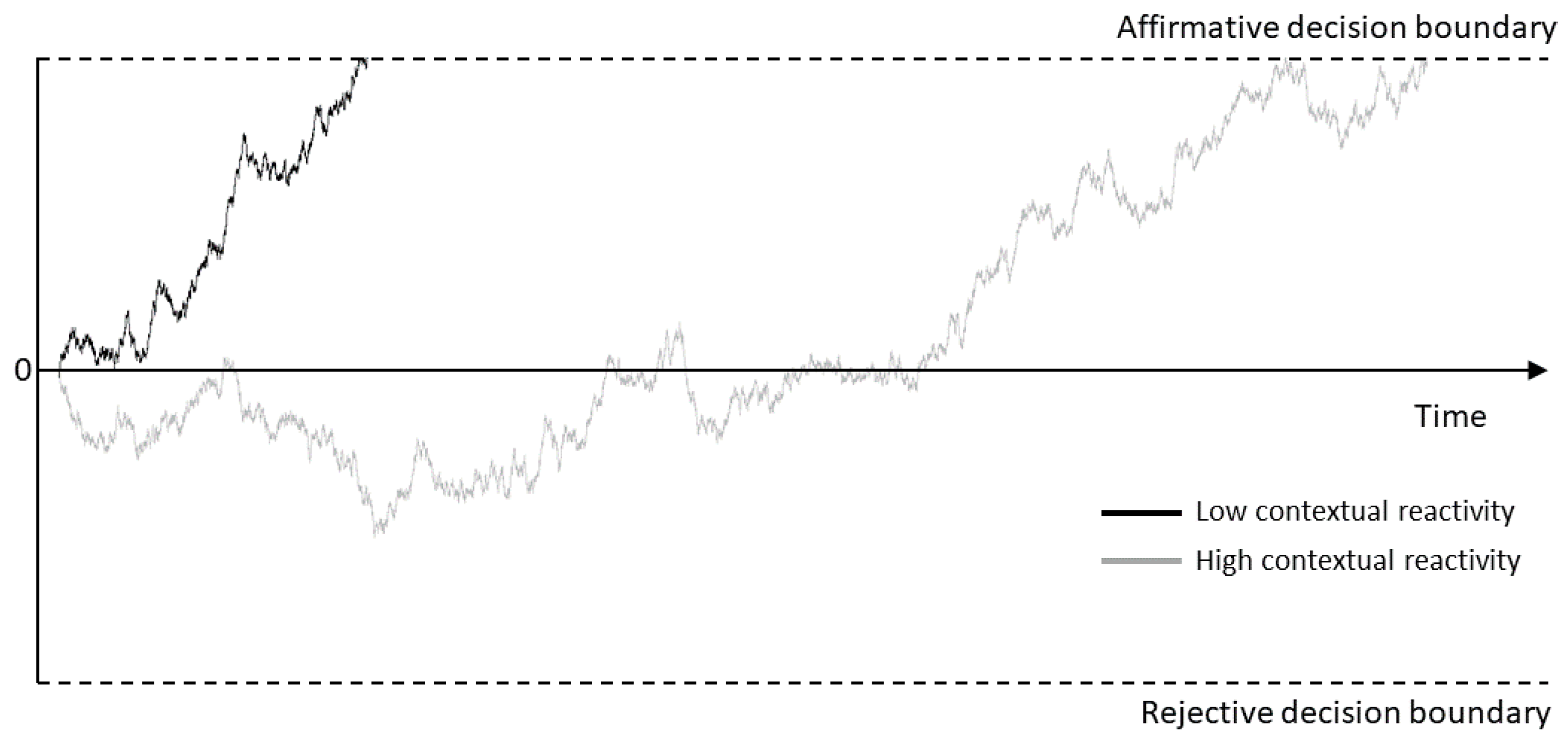
1.1.2. Information Accumulation Decision Processes in Personality and the Distance-Difficulty Hypothesis

Recently, it has been argued that the response process underlying personality inventories follows an information accumulation decision process [23,24,34]. In this process, the person accumulates evidence supporting or opposing the statement of a personality item by internally assessing past behavior and comparing that to the item statement. If enough evidence has been gathered (i.e., a decision boundary is reached), the person will make a decision based on the direction of the evidence. The time it takes to reach a decision is therefore an important indicator for this decision process.

In this information accumulation process, high contextual reactivity will be characterized by a relatively indecisive accumulation process as due to the large within-person variance in personality behavior, there will be evidence both supporting and opposing the item statement. In contrast, low contextual reactivity will be characterized by evidence that is mostly directed towards one of the options (supporting or opposing the item statement). Hence, high contextual reactivity will be defined by larger response times due to a longer period of evidence accumulation than low contextual reactivity, see Figure 2 for a graphical representation of this idea.

In addition, as the decision follows a different process for high and low contextual reactivity, the measurement parameters of the responses will be different (due to a different rate of information accumulation, and possibly, a different distance between the boundaries). Note that this is related to the notion of measurement invariance (e.g., [35,36,37]) which states that different response processes will result in different measurement parameters. Moreover, the idea above is in line with the distance–difficulty hypothesis from personality research [17,25,38,39], in which it has been shown that stable personality scores over time (i.e., small within-person variance and thus low contextual reactive) are associated with more decision certainty and faster response times than scores that show more variability over time.

As was shown by Geukes et al. [14], people may vary in their contextual reactivity across different traits. That is, Geukes et al. found that the amount of within-person variability was higher for neuroticism and openness. Here, we postulate that contextual reactivity may also depend on specific facets of a trait. For instance, a person may only show high contextual reactivity to socializing facets of extraversion, but not to other facets. In addition, it is also possible that a person only shows high contextual reactivity for specific aspects within a facet. For example, the socializing behavior of a person who is very social may be highly affected by contextual cues specific to a work environment, but not by contextual cues specific to leisure activities. This idea is also supported by the empirical work on the distance–difficulty hypothesis (discussed above) in which it has been shown that the stability of a response is highly dependent on the person (i.e., the specific position on the trait) and the item (i.e., the specific aspect of the trait/facet; e.g., [40]).

1.2. Practical Framework

Taking the above information together, the cross-sectional definition of contextual reactivity implies that high-contextual reactive responses are characterized by larger response times and by different measurement properties as compared to low-contextual reactivity responses. However, using the raw response times to make inferences about response specific contextual reactivity is challenging, as the raw response times are confounded by the item and person effects. That is, some people are on average slower than others and some items require more time than others. To make inferences about contextual reactivity, it is therefore important to distinguish between these effects and the effects of contextual reactivity on the response times.

To separate person effects, item effects, and the effects of contextual reactivity, we adopted a within-person mixture modeling approach for responses and response times [41,42,43]. In this approach, a mixture of two latent states is assumed to underlie the responses and response times of each item of a personality inventory. Each response was classified into a high contextual reactivity state or a low contextual reactivity state, based upon the response and the response time, taking the main person and main item effects into account.

Such a practical modeling framework for contextual reactivity is valuable as it provides researchers with statistical tools to enable inferences about within-subject differences in contextual reactivity while explicitly accounting for differences between persons and items. That is, the present approach will provide researchers with measures for contextual reactivity which can be used in empirical research to test hypotheses concerning personality. In addition, the approach will give insight into within-person trajectories concerning contextual reactivity underlying the responses to personality test items. Such trajectories cannot be studied using more conventional modeling approaches. In this paper, we will adopt this approach to illustrate the above advantages of distinguishing between high and low contextual reactivity. Specifically, we will apply the modeling approach to the responses and response times of the Revised Temperament and Character Inventory (TCI-R; [44]). Below, we first present the within-person mixture modeling approach and discuss how it can be used to investigate contextual reactivity, we then apply it to the TCI-R, and we end with a general discussion.

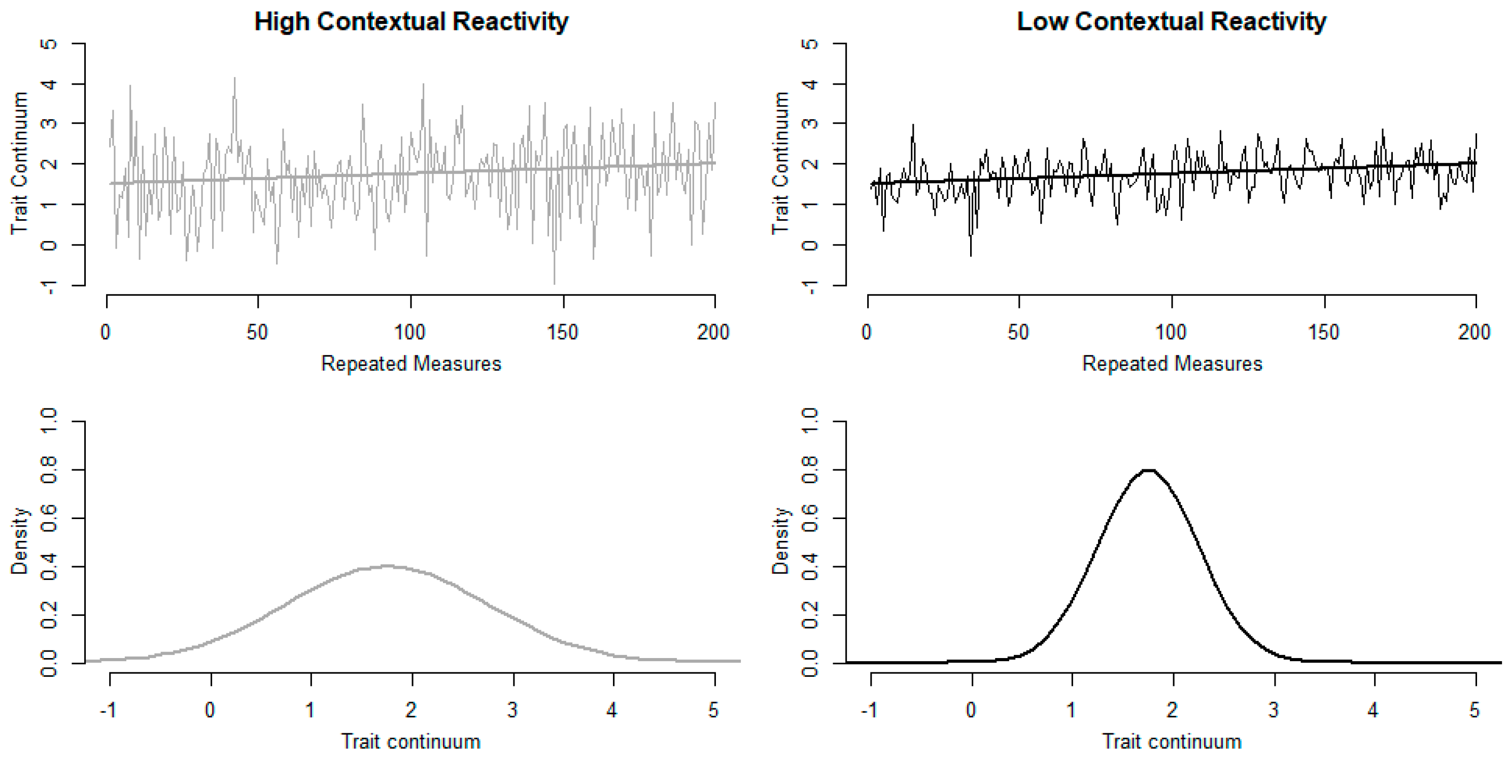
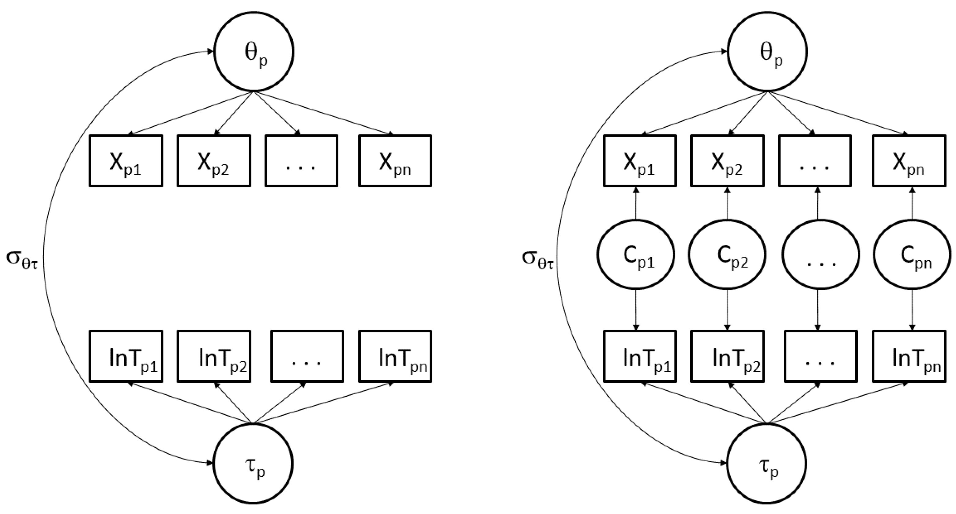
2. A Within-Person Mixture Modeling Account of Contextual Reactivity

To derive a suitable model for contextual reactivity, we first specify the hierarchical model of Van der Linden [45] as a baseline model to account for the main effects of the people and the items in responses and response times. To this end, the responses for person $p=1,\dots , N$ to item $i=1,\dots ,n$, denoted $X_{pi}$, are regressed on a latent trait variable ${\theta }_p$ resulting in item parameters, ${\alpha }_i$ (discrimination parameter) and ${\beta }_{ic}$ (category attractiveness parameter; for $c=1,\dots ,C$) and person parameters, ${\theta }_p$ (latent trait parameters), which, respectively, account for the main item effects and the main person effects. This regression can be any suitable mixed effects regression model. In this paper we use the generalized partial credit model, that is,

$$\log \left(\frac{P\left(X_{pi}=c|{\theta }_p\right)}{P\left(X_{pi}=c-1|{\theta }_p\right)}\right)={\alpha }_i{\theta }_p+{\beta }_{ic}$$

In this model, the item effects ${\alpha }_i$ and ${\beta }_{ic}$ account for differences in the measurement properties of the items. That is, the discrimination parameters ${\alpha }_i$ account for the amount of variation in the trait that is captured in the item scores, and the category attractiveness parameters ${\beta }_{ic}$ account for some categories being used more often than other categories for a given item.

Similarly, the response times for person $p$ on item $i$, $T_{pi}$, are regressed on a latent speed factor resulting in item parameters, ${\nu }_i$ (time intensities) and ${\lambda }_i$ (factor loadings), and person parameters ${\tau }_p$ (latent speed parameters). A suitable regression model for the response times ideally takes into account the skewness of the response time distribution and its natural lower bound of zero. A practical solution is to log-transform the response times and to submit these to a linear model, i.e.,:

$$E(\log T_{pi}|{\tau }_p)={\nu }_i-{\tau }_p \mathrm{with} VAR\left(\log T_{pi}|{\tau }_p\right)={\sigma }_{\epsilon i}^2$$

where ${\sigma }_{\epsilon i}^2$ is the residual variance. Note that all factor loadings are fixed to -1 in accordance with [45]. The negative sign ensures that the latent speed variable ${\tau }_p$ retains its interpretation as a speed variable with larger log-response times corresponding to smaller levels on the speed variable ${\tau }_p$. In addition, the time intensity parameter ${\nu }_i$ accounts for differences in the average log-response time to an item. This parameter is commonly referred to as the time intensity of an item. That is, some items require overall more time to be processed by the respondents, resulting in a larger mean response time for those items, for instance because the item consists of a relatively large text. To finalize the baseline model, the models for the responses and response times are connected by allowing a covariance ${\sigma }_{\theta \tau }$ between the latent variables ${\theta }_p$ and ${\tau }_p$. See left panel of Figure 3 for a graphical representation of this baseline model.

The baseline model above is a static model as it only models between-person differences. That is, latent variables ${\theta }_p$ and ${\tau }_p$ capture differences between persons in their trait and speed levels, respectively. As discussed, we are interested in modeling within-person differences as we expect within-person variance due to a person giving high-contextual reactive responses to some items and low-contextual reactive responses, which are characterized by smaller response times and different measurement properties, to others. To test this notion, we need to adapt the baseline model to account for these within-person differences. As discussed above, we will use a within-person mixture model [41]. Specifically, in the baseline model, we specify item-specific latent state variables, $C_{pi}$, with two states. The first state ($C_{pi}=0)$ is the high-contextual reactivity (HC) state which is characterized by slower response times and the second state ($C_{pi}=1)$ is the low contextual reactivity (LC) state which is characterized by faster response times, that is:

$$E\left(\log T_{pi}|{\tau }_p\right)={\nu }_i-{\mathsf{\Delta }}_{{\nu }_i}{C}_{pi}-{\tau }_p \mathrm{with} VAR\left(\log T_{pi}|{\tau }_p\right)={\sigma }_{\epsilon i}^2 \mathrm{and} \delta >0$$

where ${\mathsf{\Delta }}_{{\nu }_i}$ is a shift parameter which models the difference in time intensity (i.e., mean log-response time) between a response from the LC-state as compared to the HC-state on item $i$. To identify the LC-state to be the faster state, ${\mathsf{\Delta }}_{{\nu }_i}$ is assumed to be larger than zero. Note that the latent state variable $C_{pi}$ is item and person dependent, meaning that a person $p$ can be in state zero (HC) on item $i$, but in state one (LC) on item $i+1$. In this paper, we do not consider the possibility of having state specific residual variances ${\sigma }_{\epsilon i}^2$ (however we note that estimating state specific variances is possible in principle).

As argued above, the HC- and LC-states will not only differ in their mean response times, but they will also differ in their measurement properties (as modelled by ${\alpha }_i$ and ${\beta }_{ic}$) to reflect that both are distinct psychological variables. Therefore, in the model, these differences are accounted for by

$$\log \left(\frac{P\left(X_{pi}=c|{\theta }_p\right)}{P\left(X_{pi}=c-1|{\theta }_p\right)}\right)=({\alpha }_i+{\mathsf{\Delta }}_{{\alpha }_i}{C}_{pi}){\theta }_p+{\beta }_{ic}+{\mathsf{\Delta }}_{{\beta }_{ic}}{C}_{pi}$$

where ${\mathsf{\Delta }}_{{\alpha }_i}$ and ${\mathsf{\Delta }}_{{\beta }_{ic}}$ are shift parameters which denote the difference in, respectively, the item discrimination and the category attractiveness between the LC-state and the HC-state. Note that ${\mathsf{\Delta }}_{{\alpha }_i}$ can be interpreted as the parameter accounting for the interaction between $C_{pi}$ and ${\theta }_p$.

Besides parameters modeling the differences in discrimination, attractiveness, and time intensity between the two states of the within-person mixture model, the model contains a state size parameter which models the proportion of responses that is given from the LC-state ${\pi }_i$. That is:

$$P\left(C_{pi}=1\right)={\pi }_i$$

e.g., a state size ${\pi }_i$ of 0.9 indicates that 90% of the responses to item $i$ are given from the LC-state. See right panel of Figure 3 for a graphical representation of the within-person mixture model outlined above. Note that both the baseline and the mixture models are joint modeling approaches. That is, the models are fit to the responses and response times simultaneously (i.e., not in a two-stage or separate approach).

3. Illustration: Materials and Methods

3.1. Data

The data that are used for this paper comprise responses and response times of the Revised Temperament and Character Inventory (TCI-R; [44]), collected through computerized testing. There were 1904 participants who completed the TCI-R. Participants that failed one of the five validity items were removed from the data ($N=100$). Three participants were removed due to erroneous registration of negative response times. The data of the remaining 1801 were included in the analysis. The age of the participants ranged between 18 and 60.

The TCI-R consists of 240 personality items. Participants self-determine the degree to which they agree with the content of the item on a 5-point Likert scale, where “5” stands for “strongly agree”. The items are divided over 6 domains and 29 subscales. For each scale the characteristics of the participants, as measured through the TCI-R, can be found in

Table 1. Scales and content of the Revised Temperament and Character Inventory (TCI-R).

Domain	Scale	Characteristics of Persons Low and High on TCI-R Scale
		Low	High
Novelty seeking	NS1	Stoic rigidity	Exploratory excitability
	NS2	Reflection	Impulsiveness
	NS3	Reserve	Extravagance
	NS4	Regimentation	Disorderliness
Harm avoidance	HA1	Uninhibited optimism	Anticipatory worry
	HA2	Certainty	Fear of uncertainty
	HA3	Outgoing	Shyness with strangers
	HA4	Energy	Fatigability
Reward dependence	RD1	Indifference	Sentimentality
	RD2	Aloofness	Open to warm communication
	RD3	Distance	Attachment
	RD4	Independence	Dependence
Persistence	PS1	Laziness	Eagerness of effort
	PS2	Spoiled	Work hardened
	PS3	Underachieving	Ambitious
	PS4	Pragmatist	Perfectionist
Self-Directedness	SD1	Blaming	Responsibility
	SD2	Lack of direction	Purposefulness
	SD3	Uncreative	Resourcefulness
	SD4	Self-striving	Self-acceptance
	SD5	Pessimistic	Enlightened second nature
Cooperativeness	C1	Social intolerance	Social acceptance
	C2	Social disinterest	Empathy
	C3	Unhelpfulness	Helpfulness
	C4	Revengefulness	Compassion
	C5	Self-serving	Pure conscience
Self-Transcendence	ST1	Self-conscious	Self-forgetful
	ST2	Self-differentiation	Transpersonal identification
	ST3	Rational materialism	Spiritual acceptance

[46]. In test administration, the item order was mixed across the domains and subscales of the TCI-R but was the same across the participants. The data can be requested from the second author.

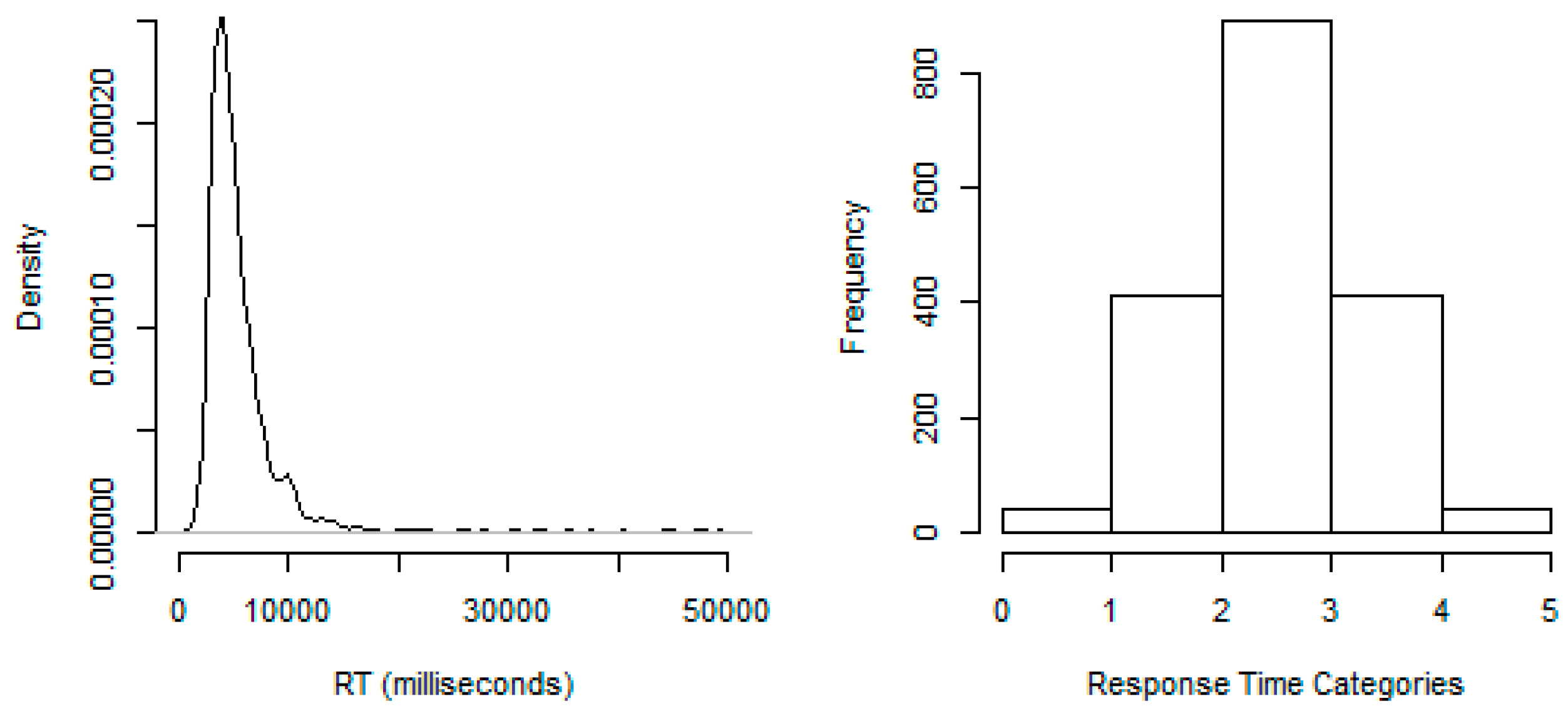
3.2. Categorizing Response Times

In the mixture model in the right panel of Figure 3, it is commonly assumed that the response times within each state are log-normally distributed (e.g., [41,43]). However, Molenaar et al. [47] showed that violations of this assumption can lead to spurious state detection (i.e., detecting two latent states where there is only one) and parameter bias. Molenaar et al. demonstrate that categorization of the continuous response times is a suitable solution for this problem, and leads to better performing models (i.e., no/less bias and no spurious state detection). Molenaar et al. found robust results for three, five, and seven response time categories. Within the current study, we therefore use 5 response time categories. We categorized the response time data following the recommendations by [48]. That is, we transformed the response times into categories using the cumulative probabilities within the standard normal distribution at −2, −2/3, 2/3, and 2. This implies cut-off values at the percentiles 2.28, 25.25, 74.75, and 97.73 of the observed response time distribution. This procedure is desirable as it results in relatively uniform information across the latent speed variable [48]. Note that due to this categorization approach, the within-person effects also become more robust to arbitrary scale properties. That is, it has been shown how traditional measures of within-person variability depend on arbitrary scale properties like the mean and the minimum/maximum of the scale (see e.g., [49]). As we use categorized response times and explicitly model each response time category (see below), these properties of the scale are taken into account and do not affect the modeling results (see [47]). Figure 4 contains the distribution of the raw and categorized response times for an example item.

3.3. Model Specification, Estimation, and Fit

The two models from Figure 3 were fit to each of the 29 TCI-R subscales separately. For the state size parameter ${\pi }_i$, we assume homogeneity of the states over items which is a common assumption in within-person mixture modeling (e.g., [50,51,52]). For the present mixture model, this assumption implies that the state sizes are equal over the items. For the purposes of the present study, we think that invariant state sizes will capture the most important patterns in the data (i.e., the overall state size). However, relaxing this assumption is possible in principle but will result in a complex model that requires (very) large sample sizes. Congruently, we specify ${\mathsf{\Delta }}_{{\alpha }_i}$, ${\mathsf{\Delta }}_{{\beta }_{ic}}$, and ${\mathsf{\Delta }}_{{\nu }_i}$ to be item invariant, that is, ${\mathsf{\Delta }}_{{\alpha }_i}={\mathsf{\Delta }}_{\alpha }$, ${\mathsf{\Delta }}_{{\beta }_{ic}}$=${\mathsf{\Delta }}_{\beta }$, and ${\mathsf{\Delta }}_{\nu i}={\mathsf{\Delta }}_{\nu }$ although we note that it is possible to estimate item specific effects (see [41]). In addition, for the categorized response times, we used a partial credit model [53]. Note that the response time model does thus not include a discrimination parameter (to follow [45]) while the model for the responses $X_{pi}$ above does include a discrimination parameter (as the responses follow a generalized partial credit model).

Thus, the mixture model that we fit to the TCI-R data is given by:

$$\log \left(\frac{P\left(T{\prime }_{pi}=c|{\tau }_p,C_{pi}\right)}{P\left(T{\prime }_{pi}=c-1|{\tau }_p,C_{pi}\right)}\right)={\nu }_{ic}-{\mathsf{\Delta }}_{\nu }{C}_{pi}-{\tau }_p$$

for the categorized responses times $T_{pi}^{\prime }$ and

$$\log \left(\frac{P\left(X_{pi}=c|{\theta }_p\right)}{P\left(X_{pi}=c-1|{\theta }_p\right)}\right)=({\alpha }_i+{\mathsf{\Delta }}_{\alpha }{C}_{pi}){\theta }_p+{\beta }_{ic}+{\mathsf{\Delta }}_{\beta }{C}_{pi}$$

for the responses. Finally, the state sizes are given by:

$$P\left(C_{pi}=1\right)=\pi$$

All models are specified in the statistical software program LatentGOLD [54]. The LatentGOLD scripts are available from www.dylanmolenaar.nl. To evaluate which model fits the data best, we consulted the Bayesian information criterion (BIC) and the Akaike information criterion (AIC). These measures are comparative fit indices, where lower values represent better model fit. Molenaar et al. [47] studied the true and false positive rates for these fit indices in selecting among similar mixture models adopted here. It was found that BIC performs acceptably and AIC is associated with an increased false positive rate in some situations. Thus, if considered together and the AIC and BIC both agree on which model is the best fitting model, this result can be trusted.

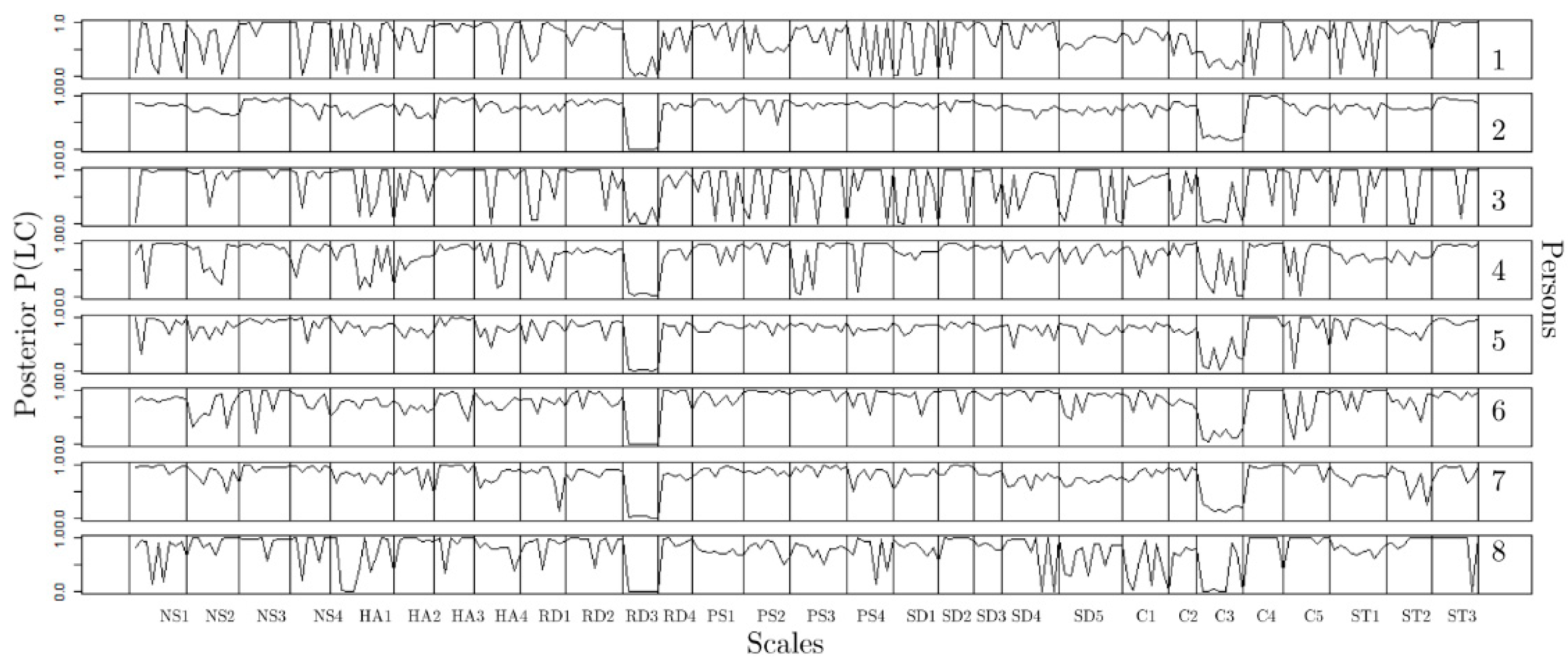
4. Illustration: Results

Table 2. Comparative fit indices and estimated correlation between $\theta$ and $\tau$ $\left({\widehat{\rho }}_{\theta \tau }\right)$ for the baseline model and the within-person mixture model.

		Baseline			Mixture
Scale	${\widehat{\mathit{\rho }}}_{\mathit{\theta }\mathit{\tau }}$	BIC	AIC	${\widehat{\mathit{\rho }}}_{\mathit{\theta }\mathit{\tau }}$	BIC	AIC
NS1	0.036	86,745.18	86,239.54	0.036	86,274.66	85,747.03
NS2	0.136	76,797.54	76,341.37	0.158	76,496.97	76,018.80
NS3	0.017	75,994.82	75,538.64	0.012	75,775.27	75,297.11
NS4	0.082	62,663.17	62,305.93	0.063	62,390.94	62,011.70
HA1	0.092	93,529.02	92,973.91	0.080	93,042.40	92,465.31
HA2	−0.004	62,894.30	62,537.06	−0.008	62,717.00	62,337.77
HA3	0.061	59,417.48	59,060.23	0.043	59,162.68	58,783.45
HA4	−0.042	69,884.02	69,477.31	−0.041	69,518.79	69,090.09
RD1	−0.045	69,330.72	68,924.01	−0.046	68,935.28	68,506.58
RD2	−0.042	84,147.09	83,641.45	0.064	83,909.34	83,381.71
RD3	−0.052	52,560.08	52,252.30	−0.048	52,439.41	52,115.14
RD4	0.091	52,492.60	52,184.82	0.084	52,386.8	52,057.04
PS1	0.161	75,821.37	75,365.19	0.143	75,367.87	74,889.71
PS2	0.000	66,910.70	66,503.98	−0.011	66,694.54	66,265.84
PS3	0.101	83,618.62	83,112.98	0.084	83,234.34	82,706.72
PS4	0.292	68,362.41	67,955.70	0.270	67,964.11	67,535.42
SD1	0.092	66,132.33	65,725.61	0.084	65,818.33	65,389.64
SD2	0.117	50,975.33	50,667.54	0.084	50,833.48	50,503.71
SD3	0.089	43,454.53	43,196.21	0.084	43,321.30	43,041.00
SD4	−0.079	88,177.16	87,671.52	−0.084	87,585.04	87,057.42
SD5	−0.148	94,303.97	93,748.86	−0.141	93,677.09	93,100.00
C1	0.071	65,185.06	64,778.35	0.064	64,977.60	64,548.90
C2	0.190	43,259.89	43,001.57	0.171	43,059.71	42,779.40
C3	0.091	65,722.88	65,316.17	0.091	65,574.89	65,151.69
C4	−0.284	57,497.02	57,139.78	−0.236	57,056.51	56,677.28
C5	−0.079	67,938.00	67,531.29	−0.083	67,598.26	67,169.56
ST1	0.233	88,067.59	87,561.95	0.211	87,528.77	87,001.15
ST2	−0.108	70,345.60	69,938.89	−0.088	69,875.43	69,446.73
ST3	−0.037	68,927.00	68,520.29	−0.025	68,552.14	68,123.45

Note: Fit indices that are presented in bold have the lowest value and thus represent the best fit.

contains the AIC and BIC fit indices of the baseline and the mixture model for the subscales of the TCI-R. As can be seen, the baseline model is rejected for all subscales in favor of the mixture model. Table 2 also includes the estimated correlation between the latent trait and latent speed variables in the two models for each scale. As can be seen the correlations differ only minorly with 20 out of the 29 scales showing a slightly larger absolute correlation in the baseline model as compared to the mixture model. This is to be expected as the main difference between the models is how the residuals are modeled. That is, in the baseline model the residuals are unmodeled, while in the mixture model, a two-states structure is imposed. The slight difference between the baseline model and the mixture model is due to the differences in measurement properties of the latent trait and latent speed variable across the states. Therefore, in the remainder, we focus on the results of the mixture model to see how the measurement properties differ across states.

First,

Table 3. Shift parameters for low contextual reactivity.

	Parameters Estimates (SE)
Scale	$\mathbf{Attractiveness} {\mathbf{\Delta }}_{\mathit{\beta }}$	$\mathbf{Discrimination} {\mathbf{\Delta }}_{\mathit{\alpha }}$	$\mathbf{Time}-\mathbf{Intensity} {\mathbf{\Delta }}_{\mathit{\nu }}$	$\mathbf{State} \mathbf{Size} \mathbf{LC} \mathit{\pi }$
NS1	0.746 (0.115)	2.339 (0.083)	0.198 (0.073)	0.845 (0.012)
NS2	−0.202 (0.070)	1.736 (0.092)	0.469 (0.076)	0.733 (0.020)
NS3	−0.181 (0.186)	2.474 (0.203)	0.701 (0.167)	0.944 (0.011)
NS4	0.312 (0.102)	2.324 (0.100)	0.235 (0.084)	0.820 (0.016)
HA1	0.106 (0.082)	1.965 (0.065)	0.449 (0.070)	0.786 (0.013)
HA2	0.051 (0.091)	2.129 (0.097)	0.491 (0.076)	0.740 (0.017)
HA3	−0.365 (0.193)	2.583 (0.186)	1.224 (0.237)	0.946 (0.009)
HA4	−0.171 (0.086)	2.076 (0.092)	0.571 (0.082)	0.782 (0.015)
RD1	0.574 (0.087)	1.893 (0.080)	0.926 (0.100)	0.771 (0.017)
RD2	−0.077 (0.115)	1.901 (0.094)	0.372 (0.111)	0.861 (0.017)
RD3	0.432 (0.313)	3.239 (0.320)	0.000 (0.000)	0.041 (0.008)
RD4	−0.153 (0.184)	1.863 (0.146)	0.567 (0.131)	0.815 (0.039)
PS1	−0.134 (0.106)	2.366 (0.087)	0.634 (0.082)	0.827 (0.011)
PS2	0.392 (0.130)	2.025 (0.107)	0.801 (0.129)	0.849 (0.016)
PS3	0.779 (0.108)	2.057 (0.089)	0.558 (0.081)	0.831 (0.014)
PS4	0.473 (0.089)	2.319 (0.092)	0.772 (0.084)	0.808 (0.012)
SD1	0.761 (0.114)	2.027 (0.110)	0.860 (0.112)	0.825 (0.015)
SD2	0.480 (0.138)	2.223 (0.149)	0.713 (0.146)	0.887 (0.025)
SD3	0.112 (0.163)	2.291 (0.119)	0.378 (0.134)	0.826 (0.020)
SD4	−0.170 (0.072)	2.069 (0.072)	0.679 (0.066)	0.775 (0.012)
SD5	0.215 (0.091)	2.285 (0.066)	0.378 (0.060)	0.740 (0.013)
C1	0.323 (0.099)	1.607 (0.118)	0.807 (0.167)	0.818 (0.020)
C2	0.859 (0.145)	2.269 (0.124)	0.609 (0.115)	0.775 (0.019)
C3	−0.634 (0.124)	1.930 (0.088)	0.006 (0.092)	0.198 (0.021)
C4	0.400 (0.079)	0.238 (0.088)	7.003 (0.432)	0.956 (0.005)
C5	1.126 (0.105)	1.945 (0.095)	0.425 (0.077)	0.786 (0.017)
ST1	0.678 (0.096)	1.949 (0.072)	0.601 (0.065)	0.756 (0.014)
ST2	−0.595 (0.101)	2.082 (0.082)	0.814 (0.081)	0.771 (0.015)
ST3	−0.281 (0.157)	2.801 (0.157)	0.460 (0.124)	0.939 (0.008)

Note: In our LatentGOLD implementation, we used $E\left(\log T_{pi}|{\tau }_p\right)={\nu }_i+{\mathsf{\Delta }}_{{\nu }_i}{C}_{pi}-{\tau }_p$ with ${\mathsf{\Delta }}_{{\nu }_i}$ < 0 which is equivalent to our model $E\left(\log T_{pi}|{\tau }_p\right)={\nu }_i-{\mathsf{\Delta }}_{{\nu }_i}{C}_{pi}-{\tau }_p$ with ${\mathsf{\Delta }}_{{\nu }_i}$ > 0, but which differs in the parameterization of ${\mathsf{\Delta }}_{{\nu }_i}$. The estimates in Table 3 are in our parameterization (i.e., with ${\mathsf{\Delta }}_{{\nu }_i}$ > 0)).

contains the parameter estimates for the shift parameters and the state size for the LC-state for the mixture model. As discussed above, the shift parameters ${\mathsf{\Delta }}_{\alpha }$, ${\mathsf{\Delta }}_{\beta }$, and ${\mathsf{\Delta }}_{\nu }$ represent the overall difference between the LC-state and the HC-state in the discrimination, attractiveness, and time intensity parameters. That is, a positive estimate of a shift parameter indicates that overall the corresponding parameter (e.g., attractiveness) is larger in the LC-state, while a negative estimate indicates that the corresponding parameter is overall smaller in the LC-state. Note that ${\mathsf{\Delta }}_{\nu }$ is restricted to be positive to identify the LC-state as the faster state.

For the shift parameters of the discrimination parameters we observe that for all subscales, the items are significantly more discriminative in the LC-state. This suggests that the relationship between the measured trait and the item-responses is stronger within the LC-state than within the HC-state. As is evident from the large estimates of ${\mathsf{\Delta }}_{\alpha }$, the item discrimination parameters in the HC-state are small, indicating that the responses in this state are discriminate poorly between people with high and low trait values. This result is understandable as the responses in the HC-state depend highly on the context and therefore contain few systematic differences. For the attractiveness parameters we observe significant differences between the states for most of the subscales. However, the direction of the difference depends on the subscale considered. For the novelty seeking (NS), harm avoidance (HA), and reward dependance (RD) domains, half of the subscales show larger attractiveness parameters in the LC-state and the other half show larger attractiveness parameters in the HC-state. For the persistence (PS), self-directedness (SD), and cooperativeness (C) domains, all but one scale shows larger attractiveness in the LC-state as compared to the HC-state, and finally, for the self-transcendence (ST) domain, two subscales show larger attractiveness in the HC-state, and one scale shows larger attractiveness in the LC-state.

For all but two subscales, the LC-state is the largest state with state size between roughly 0.7 and 0.8 for most of the subscales indicating that most responses are in the LC-state. For the RD3 and C3 subscales, the LC-state size is small (respectively, 0.041 and 0.198). However, for these two subscales, the shift parameters for the time intensities are close to zero, indicating that there is hardly a difference in mean response time between the states. This complicates the interpretation of the results in terms of a HC-state and a LC-state for these two subscales.

To illustrate what individual within-persons trajectories in state membership underlying the responses to the TCI-R look like, we depict the posterior state probability estimates of the LC-state in Figure 5 for some example participants. As can be seen, state membership dependents highly on the person, the subscale, and the item. For instance, for participant one, the responses seem to be more fluctuating between HC and LC, while for participant two, most of the responses are within the LC-state. In addition, for participant three, the responses seem to be merely within the LC-state for the NS scales and more fluctuating between LC and HC for the PS scales.

5. Discussion

In this paper, we presented a cross-section account of contextual reactivity in personality, where larger response times are indicative of responses that are more subject to contextual reactivity. We applied this idea to 29 personality dimensions, measured by the TCI-R [44]. We found two latent states to underlie the responses and response times of the TCI-R. The two latent states differ in overall response time, item discrimination, and item attractiveness, suggesting that the responses within each state measure different psychological variables. We interpreted the latent state containing the faster responses as the high contextual reactivity state and the latent state containing the slower responses as LC-state.

We observed that for all but one of the personality subscales of the TCI-R, the items have larger discrimination parameters in the low contextual reactivity state. This is in line with the idea that smaller response times indicate more stable and more precise responses [17,25,38,39] and that they have smaller underlying within-person variance in personality [1]. For the attractiveness parameters we found no systematic differences between the low and high contextual reactivity states. That is, we found the attractiveness parameters to differ across the low and high contextual reactivity states, but the direction of the difference depends on the exact subscale. Thus, contextual reactivity does not systematically relate to the item scores as for some subscales, contextually reactive responses are associated with higher item scores, and for other subscales contextual reactive responses are associated with lower item scores. As a result, these findings reflect that contextual reactivity (i.e., amount of within-person variance in personality) is theoretically distinct from the trait level (i.e., within-person mean in personality), with no systematic difference between high and low contextual reactivity on the exact item scores.

In the theoretical derivation of the practical framework for contextual reactivity, we build upon the assumption that there is an explicit distinction between personality traits and states (e.g., [22]). It should be noted that such a distinction has been not been without criticism. For instance, Ellen and Potkay [55] argued that the distinction between trait and state is arbitrary for five reasons: (1) well established trait and state questionnaires (e.g., the Adjective Check List, or Profile Of Mood States) contain a considerable amount of overlapping items; (2) in research practice, a personality measure is “declared” to measure a trait or a state by the researcher without empirical evidence; (3) researchers are unable to indicate where the state stops and the trait starts; (4) in daily life, people hardly distinguish (verbally) between trait and state; and (5) research intended to measure a trait, is sometimes post-hoc reported as research into a state. The critique by Allen and Potkay has been refuted by Zuckerman [56] who pointed to empirical studies showing that questionnaires for traits and states differ in their psychometric properties in a theoretically expected way (e.g., the test–rest reliability for traits is generally much larger than for states) and that, as would theoretically be expected, state questionnaires are vulnerable to experimental manipulation, while trait questionnaires are not. In addition, Fridhandler [57] pointed out that the trait–state distinction consists of four aspects: (1) short-term versus long-term; (2) a continuous versus a reactive manifestation; (3) a concrete versus an abstract entity; and (4) the result of situational causality versus personal causality, while Ellen and Potkay solely focus on the former two. As a result, the trait–state distinction may seem arbitrary, but if focusing on all four aspects, it is not.

In the framework proposed in this paper, we have come up with a formal distinction between traits and states, that touches mainly upon aspects one and four by Fridhandler [57]. That is, in the prosed mixture model, we assume that short-term situational specific effects ($C_{pi}$ in the model; i.e., effects that underlie specific items but not all items) characterize states and that long-term person specific effects (${\theta }_p$ in the model; i.e., the effect that underlies the data on all items of a given person) characterize the trait. As our formal framework is questionnaire independent (i.e., the formal definitions for states and traits do not depend on the exact instruction of the questionnaire) we addressed critique one and two by Ellen and Potkay [55] above. In addition, as traits and states are formally defined by, respectively, a latent trait variable ${\theta }_p$ and a latent state variable $C_{pi}$, critique three is also addressed. That is, it is made explicit what patterns in the data correspond to trait effects ${\theta }_p$ and what part corresponds to state effects $C_{pi}$. A key issue for the validity of our proposed framework is whether our distinction into traits and states is in line with the theory. However, as we have argued in the introduction section, we see a basis for this.

The idea of using the response times to operationalize contextual reactivity is intended to aid the assessment of personality in general, and the assessment of contextual reactivity in particular. That is, as illustrated in the real data application, the framework we have presented in this paper can be used to obtain measures for contextual reactivity using cross-sectional data. These measures, that is, the posterior state membership of each response, can be used in research to predict behavior more accurately. Contextual reactivity may for instance be used to predict other psychological constructs, for example, psychopathology, or, contextual reactivity may serve as a predictor for psychological resilience. In addition, contextual reactivity may be predicted from other (personality) variables by adding covariates to the mixture models as presented in this paper. Extending the model in this way is straightforward and may add to our understanding of (the distinction between) within-person variance, contextual reactivity, and personality traits in general and their relation to other variables. Either way, for these hypotheses to be tested, the assessment of contextual reactivity should be made easier, more comprehensible and less time consuming. Our proposed approach is a step forwards in this direction.

In our modeling approach, we took the hierarchical modeling framework of Van der Linden [45] as a point of departure. However, there are many other approaches to analyze responses and response times, see [58] for a recent overview. Our choice was mainly a pragmatic one: in the hierarchical model, item and person effects on responses and response times are separated in a way that is characteristic for item response theory. As a result, it is relatively straightforward to account for item and person effects to extract effects due to different item-specific latent states, which was the main aim of the present study. However, the ideas put forward in this paper are certainly amenable to other statistical modeling frameworks.

In psychometrics, most approaches to simultaneously analyze responses and response times have originated from ability measurements. As discussed for instance in [59], in ability measurement, there are (scientifically) two main reasons to add the response times to the analysis of the responses (see [60] for other, more practical reasons): (1) To increase the measurement accuracy of the latent ability underlying the responses and (2) to make inferences about differences in response processes underlying the test. In the case of personality measurement, the increase in measurement accuracy using the response times is not likely to be large as the response–response time correlations are commonly (much) lower in personality assessment as compared to ability measurement. However, response times can still be valuable to make inferences about differences in the response process underlying personality tests. For instance, response times have been used to detect faking on personality questionnaires [61] and differences in self-schema [62]. Similarly, in this paper, we have used response times to enable inferences about differences in low and high contextual reactivity. Using the responses only, these inferences are challenging. Therefore, we think that response times can also be a valuable source of information in personality assessment.

In this paper, we focused on two models, a between-person baseline model, and a mixture model with both between- and within-person effects. The issue of whether to use the baseline model or the mixture model depends on the research question. That is, the aim of this paper was to present a modeling framework which enables inferences about within-person differences in personality. If a research question is not about within-person differences in personality, the researcher is free to use a between-person modeling approach. However, the presence of within-subject differences in the data may bias the between-person differences. The biasing effects of neglecting within-person differences due to a mixture of latent states is an interesting topic on its own but it was not the focus of the present paper.

There are some limitations to the present study, that should be taken into consideration. First, we have not explicitly manipulated the context of the items. Ideally, our cross-sectional approach to assess contextual reactivity is validated by comparing the results of this approach to the results of repeated measurements. For this, one could think of a design where personality states are examined over time, and where states are measured for different contexts (e.g., experience sampling). For each person, the observed within-person variance within a specific state can then be compared to the classifications of the related responses that are measured in a cross-sectional personality inventory.

Second, we considered only two different response states to be underlying the responses. This does not, however, imply that contextual reactivity truly is a dichotomous construct. Contextual reactivity may have more than two categories or there could be a continuous latent construct underlying the responses. Here, we pragmatically use two states to facilitate interpretation (i.e., comparing a high level of contextual reactivity with a low level). We think that only two levels of contextual reactivity constitute a good interpretable approximation to contextual reactivity as a continuous variable. That is, we think that with two states, we capture the most important patterns in the data (e.g., that discrimination parameters are smaller for higher levels of contextual reactivity). Using more than two categories, or using a continuous operationalization of contextual reactivity is possible (see e.g., [63,64] for a viable approach), but these models require large sample sizes and may be more challenging to interpret.

References

1. Fleeson, W. Moving Personality beyond the Person-Situation Debate. Curr. Dir. Psychol. Sci. 2004, 13, 83–87. [Google Scholar] [CrossRef]
2. Fleeson, W. The production mechanisms of traits: Reflections on two amazing decades. J. Res. Pers. 2017, 69, 4–12. [Google Scholar] [CrossRef]
3. Ardelt, M. Still Stable after All These Years? Personality Stability Theory Revisited. Soc. Psychol. Q. 2000, 63, 392. [Google Scholar] [CrossRef]
4. McCrae, R.R.; Costa, P.T. Self-concept and the stability of personality: Cross-sectional comparisons of self-reports and ratings. J. Pers. Soc. Psychol. 1982, 43, 1282–1292. [Google Scholar] [CrossRef]
5. Costa, P.T., Jr.; McCrae, R.R. Still stable after all these years: Personality as a key to some issues in adulthood and old age. Life Span Dev. Behav. 1980, 3, 65–102. [Google Scholar]
6. McCrae, R.R.; Costa, P.T. The Stability of Personality: Observations and Evaluations. Curr. Dir. Psychol. Sci. 1994, 3, 173–175. [Google Scholar] [CrossRef]
7. Moss, H.A.; Susman, E.J. Constancy and change in human development. Longitud. Study Personal. Dev. 1980, 530–595. [Google Scholar] [CrossRef]
8. Cervone, D.; Shoda, Y. Beyond Traits in the Study of Personality Coherence. Curr. Dir. Psychol. Sci. 1999, 8, 27–32. [Google Scholar] [CrossRef]
9. Fleeson, W. Toward a structure- and process-integrated view of personality: Traits as density distributions of states. J. Pers. Soc. Psychol. 2001, 80, 1011–1027. [Google Scholar] [CrossRef]
10. Fleeson, W. Studying personality processes: Explaining change in between-persons longitudinal and within-person multilevel models. In Handbook of Research Methods in Personality Psychology; Robins, R.W., Fraley, C., Krueger, R.F., Eds.; Guilford Press: New York, NY, USA, 2007; pp. 523–542. [Google Scholar] [CrossRef]
11. Mõttus, R.; Allerhand, M.; Johnson, W. Computational Modeling of Person-Situation Transactions. In The Oxford Handbook of Psychological Situations; Oxford University Press: Oxford, UK, 2017. [Google Scholar] [CrossRef]
12. Mõttus, R.; Epskamp, S.; Francis, A. Within- and between individual variability of personality characteristics and physical exercise. J. Res. Pers. 2017, 69, 139–148. [Google Scholar] [CrossRef] [Green Version]
13. Jones, A.B.; Brown, N.A.; Serfass, D.G.; Sherman, R.A. Personality and density distributions of behavior, emotions, and situations. J. Res. Pers. 2017, 69, 225–236. [Google Scholar] [CrossRef]
14. Geukes, K.; Nestler, S.; Hutteman, R.; Küfner, A.C.; Back, M.D. Trait personality and state variability: Predicting individual differences in within- and cross-context fluctuations in affect, self-evaluations, and behavior in everyday life. J. Res. Pers. 2017, 69, 124–138. [Google Scholar] [CrossRef]
15. Steinberg, L. The consequences of pairing questions: Context effects in personality measurement. J. Pers. Soc. Psychol. 2001, 81, 332–342. [Google Scholar] [CrossRef] [PubMed]
16. Dalal, R.S.; Meyer, R.D.; Bradshaw, R.P.; Green, J.P.; Kelly, E.D.; Zhu, M. Personality Strength and Situational Influences on Behavior. J. Manag. 2015, 41, 261–287. [Google Scholar] [CrossRef]
17. Ferrando, P.J.; Lorenzo-Seva, U. An Item Response Theory Model for Incorporating Response Time Data in Binary Personality Items. Appl. Psychol. Meas. 2007, 31, 525–543. [Google Scholar] [CrossRef]
18. Pervin, L.A. A free-response description approach to the analysis of person-situation interaction. In The Psychology of Social Situations; Furnham, A., Argyle, M., Eds.; Elsevier: Amsterdam, Netherlands, 1981; pp. 40–55. [Google Scholar] [CrossRef]
19. Monson, T.C.; Hesley, J.W.; Chernick, L. Specifying when personality traits can and cannot predict behavior: An alternative to abandoning the attempt to predict single-act criteria. J. Pers. Soc. Psychol. 1982, 43, 385–399. [Google Scholar] [CrossRef]
20. Harris, K.B.; Sawyer, C.R.; Behnke, R.R. Predicting Speech State Anxiety from Trait Anxiety, Reactivity, and Situational Influences. Commun. Q. 2006, 54, 213–226. [Google Scholar] [CrossRef]
21. Watson, D.; Clark, L.A.; Harkness, A.R. Structures of personality and their relevance to psychopathology. J. Abnorm. Psychol. 1994, 103, 18–31. [Google Scholar] [CrossRef]
22. Hamaker, E.L.; Nesselroade, J.R.; Molenaar, P.C. The integrated trait–state model. J. Res. Pers. 2007, 41, 295–315. [Google Scholar] [CrossRef]
23. Tuerlinckx, F.; De Boeck, P. Two interpretations of the discrimination parameter. Psychometrika 2005, 70, 629–650. [Google Scholar] [CrossRef]
24. Van Der Maas, H.L.J.; Molenaar, D.; Maris, G.; Kievit, R.A.; Borsboom, D. Cognitive psychology meets psychometric theory: On the relation between process models for decision making and latent variable models for individual differences. Psychol. Rev. 2011, 118, 339–356. [Google Scholar] [CrossRef] [PubMed] [Green Version]
25. Kuncel, R.B. Response Processes and Relative Location of Subject and Item. Educ. Psychol. Meas. 1973, 33, 545–563. [Google Scholar] [CrossRef]
26. Eysenck, H.J. Cicero and the state-trait theory of anxiety: Another case of delayed recognition. Am. Psychol. 1983, 38, 114–115. [Google Scholar] [CrossRef]
27. Hertzog, C.; Nesselroade, J.R. Beyond Autoregressive Models: Some Implications of the Trait-State Distinction for the Structural Modeling of Developmental Change. Child Dev. 1987, 58, 93–109. [Google Scholar] [CrossRef] [PubMed]
28. Steyer, P.D.R.; Schmitt, M.; Eid, M. Latent state–trait theory and research in personality and individual differences. Eur. J. Pers. 1999, 13, 389–408. [Google Scholar] [CrossRef]
29. Spielberger, C.D.; Sydeman, S.J. State Trait Anxiety Inventory and State-Trait Anger Expression Inventory. In The Use of Psychological Tests for Treatment Planning and Outcome Assessment; Maruish, M.E., Ed.; Lawrence Erlbaum Associates: Hillsdale, NJ, USA, 1994; pp. 292–321. [Google Scholar] [CrossRef]
30. Costa, P.T.; Herbst, J.H.; McCrae, R.R.; Siegler, I.C. Personality at midlife: Stability, intrinsic maturation, and response to life events. Assessment 2000, 7, 365–378. [Google Scholar] [CrossRef]
31. McCrae, R.R.; Costa, P.T., Jr.; Terracciano, A.; Parker, W.D.; Mills, C.J.; De Fruyt, F.; Mervielde, I. Personality trait development from age 12 to age 18: Longitudinal, cross-sectional and cross-cultural analyses. J. Pers. Soc. Psychol. 2002, 83, 1456–1468. [Google Scholar] [CrossRef]
32. Nesselroade, J.R. Interindividual differences in intraindividual change. Best Methods Anal. Chang. Recent Adv. Unanswered Quest. Future Dir. 1991, 92–105. [Google Scholar] [CrossRef]
33. Nesselroade, J.R. Intraindividual Variability in Development within and Between Individuals. Eur. Psychol. 2001, 6, 187–193. [Google Scholar] [CrossRef]
34. Tuerlinckx, F.; Molenaar, D.; van der Maas, H.L.J. Diffusion-based item response modeling. In Handbook of Modern Item Response Theory Volume 1; van der Linden, W.J., Ed.; Chapman and Hall/CRC Press: Boca Raton, FL, USA, 2016; pp. 283–300. [Google Scholar] [CrossRef]
35. Meredith, W. Notes on factorial invariance. Psychometrika 1964, 29, 177–185. [Google Scholar] [CrossRef]
36. Meredith, W. Measurement invariance, factor analysis and factorial invariance. Psychometrika 1993, 58, 525–543. [Google Scholar] [CrossRef]
37. Mellenbergh, G.J. Item bias and item response theory. Int. J. Educ. Res. 1989, 13, 127–143. [Google Scholar] [CrossRef]
38. Fekken, G.; Holden, R.R. Response latency evidence for viewing personality traits as schema indicators. J. Res. Pers. 1992, 26, 103–120. [Google Scholar] [CrossRef]
39. Holden, R.R.; Fekken, G.C.; Cotton, D.H. Assessing psychopathology using structured test-item response latencies. Psychol. Assess. 1991, 3, 111–118. [Google Scholar] [CrossRef]
40. Kuncel, R.B. The Subject-Item Interaction in itemmetric Research. Educ. Psychol. Meas. 1977, 37, 665–678. [Google Scholar] [CrossRef]
41. Molenaar, D.; Oberski, D.; Vermunt, J.; De Boeck, P. Hidden Markov Item Response Theory Models for Responses and Response Times. Multivar. Behav. Res. 2016, 51, 606–626. [Google Scholar] [CrossRef]
42. Schnipke, D.L.; Scrams, D.J. Modeling Item Response Times With a Two-State Mixture Model: A New Method of Measuring Speededness. J. Educ. Meas. 1997, 34, 213–232. [Google Scholar] [CrossRef]
43. Wang, C.; Xu, G. A mixture hierarchical model for response times and response accuracy. Br. J. Math. Stat. Psychol. 2015, 68, 456–477. [Google Scholar] [CrossRef]
44. Cloninger, C.R.; Przybeck, T.R.; Svrakic, D.M.; Wetzel, R.D. The Temperament and Character Inventory (TCI): A Guide to Its Development and Use; Center for the Psychobiology of Personality, Washington University: St. Louis, MI, USA, 1999. [Google Scholar] [CrossRef]
45. Van Der Linden, W.J. A Hierarchical Framework for Modeling Speed and Accuracy on Test Items. Psychometrika 2007, 72, 287–308. [Google Scholar] [CrossRef] [Green Version]
46. Mochcovitch, M.D.; Nardi, A.E.; Cardoso, A. Temperament and character dimensions and their relationship to major depression and panic disorder. Rev. Bras. Psiquiatr. 2012, 34, 342–351. [Google Scholar] [CrossRef] [Green Version]
47. Molenaar, D.; Bolsinova, M.; Vermunt, J.K. A semi-parametric within-subject mixture approach to the analyses of responses and response times. Br. J. Math. Stat. Psychol. 2018, 71, 205–228. [Google Scholar] [CrossRef] [PubMed]
48. Molenaar, D.; Rózsa, S.; Bolsinova, M. A heteroscedastic hidden Markov mixture model for responses and categorized response times. Behav. Res. Methods 2019, 51, 676–696. [Google Scholar] [CrossRef] [PubMed]
49. Mestdagh, M.; Pe, M.; Pestman, W.; Verdonck, S.; Kuppens, P.; Tuerlinckx, F. Sidelining the mean: The relative variability index as a generic mean-corrected variability measure for bounded variables. Psychol. Methods 2018, 23, 690–707. [Google Scholar] [CrossRef] [PubMed]
50. Bacci, S.; Pandolfi, S.; Pennoni, F. A comparison of some criteria for states selection in the latent Markov model for longitudinal data. Adv. Data Anal. Classif. 2014, 8, 125–145. [Google Scholar] [CrossRef] [Green Version]
51. Gudicha, D.W.; Schmittmann, V.D.; Vermunt, J.K. Power computation for likelihood ratio tests for the transition parameters in latent Markov models. Struct. Equ. Modeling Multidiscip. J. 2016, 23, 234–245. [Google Scholar] [CrossRef]
52. Zucchini, W.; MacDonald, I.L.; Langrock, R. Hidden Markov Models for Time Series: An Introduction Using R; Chapman and Hall/CRC: Londen, UK, 2016. [Google Scholar] [CrossRef]
53. Masters, G.N. Partial credit model. In Handbook of Item Response Theory, Volume One; Chapman and Hall/CRC: Londen, UK, 2016; pp. 137–154. [Google Scholar] [CrossRef]
54. Vermunt, J.K.; Magidson, J. Technical Guide for Latent GOLD 5.0: Basic, Advanced, and Syntax; Statistical Innovations Inc.: Belmont, MA, USA, 2013. [Google Scholar]
55. Allen, B.P.; Potkay, C.R. On the arbitrary distinction between states and traits. J. Personal. Soc. Psychol. 1981, 41, 916. [Google Scholar] [CrossRef]
56. Zuckerman, M. The distinction between trait and state scales is not arbitrary: Comment on Allen and Potkay’s “On the arbitrary distinction between traits and states”. J. Personal. Soc. Psychol. 1983, 44, 1083–1086. [Google Scholar] [CrossRef]
57. Fridhandler, B.M. Conceptual note on state, trait, and the state-trait distinction. J. Pers. Soc. Psychol. 1986, 50, 169–174. [Google Scholar] [CrossRef]
58. De Boeck, P.; Jeon, M. An Overview of Models for Response Times and Processes in Cognitive Tests. Front. Psychol. 2019, 10, 102. [Google Scholar] [CrossRef] [Green Version]
59. Molenaar, D. The Value of Response Times in Item Response Modeling. Meas. Interdiscip. Res. Perspect. 2015, 13, 177–181. [Google Scholar] [CrossRef]
60. Orange, A.; Gorin, J.; Jia, Y.; Kerr, D. Collecting, analysing, and interpreting response time, eye tracking and log data. In Validation of Score Meaning for the Next Generation of Assesments; Ercikan, K., Pellegrino, J.W., Eds.; Routledge: New York, NY, USA, 2017; pp. 39–51. [Google Scholar]
61. Holden, R.R.; Kroner, D.G. Relative efficacy of differential response latencies for detecting faking on a self-report measure of psychopathology. Psychol. Assess. 1992, 4, 170. [Google Scholar] [CrossRef]
62. Akrami, N.; Hedlund, L.-E.; Ekehammar, B. Personality scale response latencies as self-schema indicators: The inverted-U effect revisited. Pers. Individ. Differ. 2007, 43, 611–618. [Google Scholar] [CrossRef]
63. Bolsinova, M.; De Boeck, P.; Tijmstra, J. Modelling Conditional Dependence between Response Time and Accuracy. Psychometrika 2017, 82, 1126–1148. [Google Scholar] [CrossRef] [PubMed]
64. Bolsinova, M.; Molenaar, D. Modeling Nonlinear Conditional Dependence between Response Time and Accuracy. Front. Psychol. 2018, 9, 1525. [Google Scholar] [CrossRef]
Figure 1. State variation and trait change (upper plots), and the within-person distribution of states (lower plots) for high contextual reactivity (left) and low contextual reactivity (right).
Psych 02 00019 g001
Figure 2. Information accumulation process for person with low and high contextual reactivity.
Psych 02 00019 g002
Figure 3. Graphical (simplified) representation of the baseline model (left) and the within-persons mixture model (right). Note that the residual variances for l n T p i are omitted for clarity.
Psych 02 00019 g003
Figure 4. The raw response time distribution and the corresponding categorized response time distribution for an example item of the TCI-R.
Psych 02 00019 g004
Figure 5. The posterior probability of a response being classified within the LC-state for each item within each scale and 8 different people.
Psych 02 00019 g005