Article

Study on Friction in Automotive Shock Absorbers Part 1: Friction Simulation Using a Dynamic Friction Model in the Contact Zone of an FEM Model

Automotive Engineering Group, Department of Mechanical Engineering, TU Ilmenau, Ehrenbergstraße 15, 98693 Ilmenau, Germany
*
Author to whom correspondence should be addressed.
Submission received: 15 March 2021 / Revised: 23 April 2021 / Accepted: 11 May 2021 / Published: 14 May 2021
(This article belongs to the Special Issue Dynamics and Control of Automated Vehicles)

Abstract

:
The important change in the transition from partial to high automation is that a vehicle can drive autonomously, without active human involvement. This fact increases the current requirements regarding ride comfort and dictates new challenges for automotive shock absorbers. There exist two common types of automotive shock absorber with two friction types: The intended viscous friction dissipates the chassis vibrations, while the unwanted solid body friction is generated by the rubbing of the damper’s seals and guides during actuation. The latter so-called static friction impairs ride comfort and demands appropriate friction modeling for the control of adaptive or active suspension systems. In this article, a simulation approach is introduced to model damper friction based on the most friction-relevant parameters. Since damper friction is highly dependent on geometry, which can vary widely, three-dimensional (3D) structural FEM is used to determine the deformations of the damper parts resulting from mounting and varying operation conditions. In the respective contact zones, a dynamic friction model is applied and parameterized based on the single friction point measurements. Subsequent to the parameterization of the overall friction model with geometry data, operation conditions, material properties and friction model parameters, single friction point simulations are performed, analyzed and validated against single friction point measurements. It is shown that this simulation method allows for friction prediction with high accuracy. Consequently, its application enables a wide range of parameters relevant to damper friction to be investigated with significantly increased development efficiency.

1. Introduction

Modern active and adaptive chassis setups enable the achievement of both a high comfort level and the potential for high driving dynamics, even on rough roads or fast changing road properties, and are relevant for automated driving [1]. The related chassis control algorithms require appropriate models to realistically describe the physical behavior of the contributing chassis components.
This article focuses on the modeling of the shock absorber’s friction behavior. Besides its main task of damping oscillations via viscous fluid friction, the automotive shock absorber’s force-speed behavior is also characterized by the solid friction of its seals and guides rubbing against their counterparts. While the viscous fluid friction is proportional to the actuation speed and thus zero at zero speed, the seal friction acts roughly as a force offset, which causes a breakaway force to be exceeded before the shock absorber starts moving. In conventional chassis designs, this so-called static friction impairs ride comfort and driving safety, because the damper acts like a non-deformable part as long as the actuation force is smaller than the static friction. Since automotive shock absorbers are usually mounted in parallel to the suspension springs, this behavior deactivates the whole suspension system, resulting in a direct transfer of each transient wheel displacement to the cabin and thus high acceleration and acceleration changes to the cabin and to the driver. That is why the presence of static damper friction increases the requirements to appropriate damper friction modeling for the control algorithms of adaptive or active suspensions [2]. Dependent on the design of both the shock absorber and the seal design, this friction behavior is quite complex, dependent on various parameters, and therefore hard to predict. Since the static friction’s quantitative magnitude is not significantly increasing apart of the very-low speed range, it becomes irrelevant at high speeds due to its then very small contribution to the overall damping force [3]. That is why this study focuses on the very-low speed range.
Since friction in the shock absorber is mainly determined by the seals and their counterparts, most of the state of this research field is dedicated to seal friction. This topic is part of the area of rubber/metal friction, where e.g., [3,4,5] present comprehensive summaries of the fundamental state of research. The seals, which are commonly made from elastomers (e.g., nitrile butadiene rubber—NBR or fluoroelastomer rubber—FKM) or plastomers (e.g., polytetrafluoroethylene, PTFE), share more or less oil-lubricated topology with their commonly metal counterparts, which leads to interfering friction mechanisms as soon as relative motion occurs. Mainly the combination of deformation friction, adhesion friction and viscous fluid friction is determining the dynamic friction behavior of this setup [3]. The transient behavior of the surface’s asperities and the evolution of the lubrication film during motion changes determine the appearance of transient friction effects, like pre-sliding displacement, frictional lag, non-reversible friction characteristics, or rising static friction [3,6,7]. The investigation of real friction behavior led to the development of various friction models, starting with static friction models, which consider Coulomb’s normal force dependence, Stribeck’s lubrication states or Karnopp’s stick-slip switching [7,8,9]. To overcome the basic weaknesses of these static friction models, the discontinuity at zero speed and the overall neglect of the above-mentioned transient friction effects, dynamic friction models were developed, starting with Dahl [10], the subsequent LuGre model [11] with its various enhancements (e.g., the elasto-plastic friction model [12,13] or the Leuven integrated friction model [14]) up to transition to physics-based friction models (e.g., the generalized Maxwell slip model [15]). All these dynamic friction models share the property of being defined by a heuristically determined set of equations which are parameterized by reference measurements. Friction models, which are determined by actual physical parameters (e.g., oil viscosity and surface tension, asperity stiffness and geometry, etc.) are so-called physics-based friction models, which allow for even better description of the friction behavior, especially of the lubrication part (e.g., direct or inverse elasto-hydrodynamic lubrication [16,17] up to two-way coupled fluid structure interaction). The major disadvantage of these physics based friction models is the significantly increased computational effort, which limits their use case to special applications even today.
The research contribution of the proposed study is a hybrid damper friction modeling approach combining both the advantages of physical modeling and the low computational requirements of dynamic friction models. This approach is capable of considering both macroscopic friction-related parameters (e.g., damper setup, seal design, transient material properties, operating conditions) and microscopic friction-related parameters (e.g., surface qualities, lubrication state) by use of a dynamic friction model applied to the contact zone of a three-dimensional (3D) structural FEM setup. This approach is therefore capable to characterize the shock absorber’s friction behavior without performing extensive experiments on real prototypes. Through its comparatively low computational requirements, it allows for fast performance of wide parameter studies and the application in development and testing of ride control algorithms.
This article is structured as follows: Section 2 introduces the real shock absorber which is used as a reference for the presented study. Section 3 is concerned with the general simulation approach based on the intended model application. The simulation setup is introduced in Section 4, aiming to give a detailed setup documentation for appropriate result discussion. Section 5 presents and discusses these simulation results, followed by Section 6 with a brief summary and interpretation of the achievements of this research.

2. Reference Damper Introduction

The investigations during this research are carried out on a representative reference damper. This automotive shock absorber is a common series mono tube damper intended for rear axle application in compact cars. Its characterizing dimensions are an 11 mm outer diameter rod and a 36 mm inner diameter tube. A partially simplified drawing is presented in Figure 1, showing overview on the left side and magnified depictions of the three single friction points (A) rod guide assembly/rod, (B) piston/tube, and (C) floating piston/tube. As demonstrated in the figure, the seals penetrate their respective counterparts because this depiction shows the undeformed state representing all geometries before mounting.
The rod guide assembly/rod friction point (A) separates the damper’s oil volume from the environment, mainly through the rubber oil seal (6) in contact to the rod (2), which is made from chrome-plated steel. The oil seal is supported by the static seal (7), another rubber part and designed to transmit the damper’s inner static pressure to a mainly radial pre-tension force on the oil seal. The bronze-made bearing (3), coated with a friction-minimizing PTFE layer, is located above the oil seal to support the lateral forces to the damper. The outer closing is the scraper (1) which prevents dirt from entering the rod guide assembly, and simultaneously ensures the lubrication of the bearing with oil that passed the oil seal or an initial greasing. The scraper is also a rubber part with a pre-tensioning ingrained spring, which is not directly contributing to the scraper/rod friction. All parts of the rod guide assembly are mounted on the aluminum housing (4) which is closed with a steel closing. The sealing against the tube (12) is ensured by a rubber O-ring (5), the fixation to the tube by a roll closing (series damper) or a screwed cap (take apart damper), both not depicted in Figure 1 to maintain clarity.
The piston/tube friction point (B) prevents the oil from bypassing the piston’s bores and valve package (11) to ensure appropriate damping. It also acts as the second support to lateral forces applied to the damper. To achieve both proper tightness and low friction against the tube (12) under lateral forces, the seal is carried out as a PTFE band (10) mounted to the piston (9). Since the piston’s bores together with the valve package are generating a hydrodynamic damping force, which is overlaying the friction measurement, the valve package is generally not considered within this research.
The floating piston/tube friction point (C) seals the oil volume against the volume compensating and pressurized gas volume. This is done by a rubber O-ring (14), which is mounted to a glass fiber reinforced plastics floating piston (13) and seals against the tube (12). This pressure is transferred via the floating piston to the oil volume, thus creating a nominal operating pressure of 25 bar inside the damper.

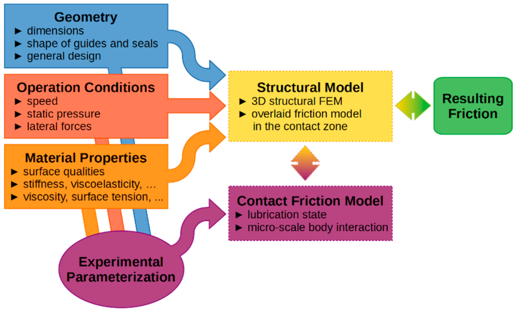
3. Simulation Methodology

Friction is generated in the single friction points (A), (B) and (C) as introduced above. Since these single friction points show differences in geometry, material, operating conditions and lubrication state, it is assumed to be feasible to divide the overall damper behavior in individual friction contributions and summarize their friction behavior in the end. Given that friction is highly dependent on the geometry and material properties of the contact surfaces it is necessary to take both of these aspects into account. To facilitate the exchange or modification of the geometry of the friction-related parts, the setup is based on CAD data. Since body–body interaction between the friction-related and also between the non-friction-related parts are defining the contact generation, contact release and contact deformation, this behavior is modeled in the 3D FEM software Ansys Mechanical, which brings a GUI with it and answers therefore the need for an easy-to-use interface in daily engineering. While end-user FEM software is usually only capable of treating the solid body part of the friction contact, fluid film formation and behavior in the contact zone is crucial for the description of lubricated friction contacts. To consider this in the overall simulation approach, an additional method must be implemented and coupled to the FEM simulation, since both interact with each other. Possible solutions for this problem start at simply adding a static friction model to the contact zone, continue with dynamic friction models or very simplified fluid calculations (e.g., EHL as proposed by [18]) and end with fully transient three dimensional CFD, which in combination with the FEM part leads to a Fluid Structure Interaction (FSI) problem.
During this research it became swiftly apparent that both FSI and EHL were not feasible. That is, the FSI implementation led to an unacceptable compromise of geometry and boundary condition simplifications versus computational effort. The EHL implementation was designed so as to solve its fluid equations by the internal solver of the FEM software with the aim of keeping the coupling effort as low as possible. However, this attempt failed due to an incomplete documentation of the FE solver’s behavior and treatment of user-defined finite elements. An alternative, namely the coupling of an additional external solver to these calculations, would demand significantly more development effort than possible within this research. Finally, EHL does not fit the problem description because of its main application in the elasto-hydrodynamic friction regime. Since actuation speed is very low in damper friction measurements and the turn-around points are of special interest, the relative speed in the contact zone is often near to zero. Thus, the mandatorily applied solid and mixed dynamic friction model to the EHL approach would be most significant during most parts of the simulation. That is why a dynamic friction model is chosen as the best possible modeling approach. Summarizing, only with the exclusive implementation of a dynamic friction model to the FEM software it is possible:
  • To achieve sufficiently low requirements for computing power and storage, and a sufficiently low setup effort to achieve usability in every-day engineering;
  • To consider three-dimensional influences, e.g., consideration of tangential seal stress, lateral forces or production non-uniformities;
  • To consider all friction states in one friction model;
  • To consider friction-induced seal deformation with full coupling to the deformation-induced contact pressure and contact area changes.
A general overview over the solution approach of this research is visualized in Figure 2. Whereas the macro-scale parameters from the three parameter groups geometry, operation conditions and material properties are directly put into the FEM’s boundary conditions, their micro-scale parameters are represented by the contact friction model’s parameter set which is experimentally obtained. Since the structural FEM model influences the contact friction model’s boundary conditions, and the friction generated by the contact friction model influences solid body deflection in the structural FEM model, there is a two-way coupling between these blocks in Figure 2. That is also the case for the finally resulting overall friction behavior.

4. Simulation Setup

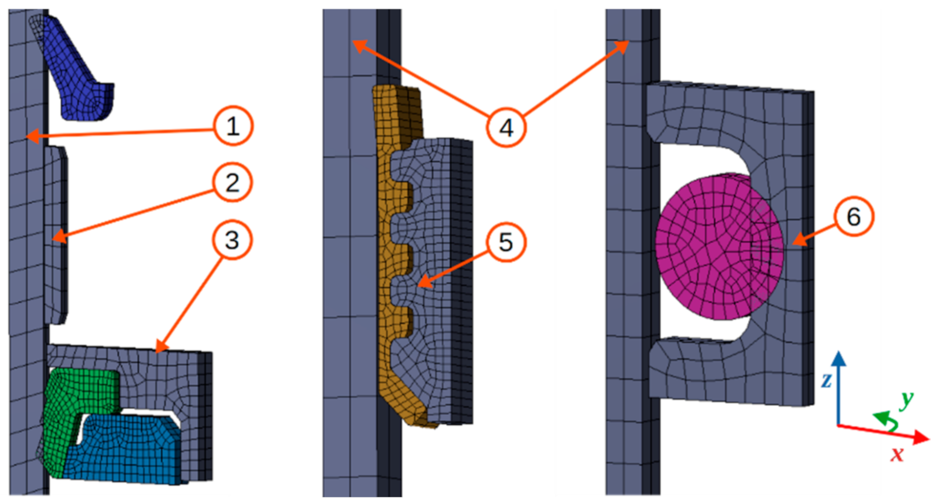
4.1. Geometry Abstraction and Spatial Discretization

For the definition of a reference case, and to keep the transfer process from CAD files to the FEM setup as straightforward as possible, the original CAD data shown in Figure 1 are used almost unmodified in the simulation. The only changes applied are the addition of small radii where the seal’s geometry shows sharp edges, and the elimination of the infused spring of the scraper. The sizes of the radii were chosen based on microscopic measurements performed on a 3D laser scanning microscope. To further simplify the simulation geometry, and therefore reducing the computational effort, rotational symmetry is assumed for all parts. To maintain the consideration of three-dimensional effects like tangential seal tensions, the geometry is not simplified to 2D, but only a small part of the actual perimeter (a wedge) is modeled by use of rotational symmetry boundary conditions on the cutting surfaces.
The necessity of modeling at least tangential seal tensions for friction simulations becomes evident through the comparison of two model approaches of the floating piston/tube contact as depicted in Figure 3. There, on the left side, the model is set up from a 4° wedge of the original CAD geometry, while the right side model is set up as a 2.5 D model of the original CAD geometry, where 2.5 D means a flat FEM setup with a mesh consisting of only one element layer. Both sides of Figure 3 show a steady state which fulfills the contact definition and which shows the equivalent stress distribution after 30 min still-standing time for appropriate O-ring material relaxation. The illustration demonstrates that the stress distribution of the 2.5 D setup is axisymmetric according to the vertical center line of the O-ring, while the stress distribution of the 4° wedge setup is visibly asymmetric. This asymmetry is caused by the general widening of the O-ring’s diameter due to its initial shape (see Figure 1C). In this illustration, the O-ring penetrates the floating piston, but not the tube, which causes the aforementioned diameter widening while fulfilling the contact definition. This is not considered in the 2.5 D setup, where the O-ring slice has no relation or connection to its perimeter. The consequence of the general widening are tangential seal tensions, which cause a much higher overall equivalent stress level in the 4° wedge setup with a much smaller stress maximum, as compared to the 2.5 D setup. Since the general widening of the O-ring also occurs in reality during the mounting process, the 4° wedge results are considered much more realistic than the 2.5 D results.
Even if the internal stress distribution is not directly affecting the friction behavior in the contact zone, it affects the contact area and contact normal force that are created between the O-ring and its counterparts. The related FEM calculation results of the contact area A O T and the circumferential contact normal force F N O T are also shown in Figure 3, both projected to the full perimeter of each setup. A O T of the 2.5 D setup is 28% too large compared to the wedge setup, which is caused by the lower lateral forces due to the aforementioned general diameter widening. In this too large contact area, an also significantly too large contact normal force is reached. The friction force is calculated within this research from the tangential shear stress τ f r i c derived from a friction coefficient μ dependent on several parameters, contact pressure p and contact surface A according to Equation (1). As a consequence, the friction force of the 2.5 D setup would be significantly overestimated.
F f r i c = τ f r i c A O T = μ p O T A O T = μ F N
whereas the modeling of tangential seal stresses is always required to determine the contact pressure with sufficient accuracy, the modeling of non-rotational symmetric effects is possible with full-perimeter approaches. To achieve a commonly usable reference friction simulation model at unit level with the lowest possible computational requirements for fast application and solving, the rotational symmetric wedge approach is chosen. This wedge approach provides sufficiently low computational effort, but considers three-dimensional effects to the desired extent. Additionally, the enhancement of the rotational symmetric approach to an area-symmetric half-model is very simple and straightforward.
The final geometry abstraction is depicted for each friction point in Figure 4. As shown in this illustration, additional simplifications are applied to all parts of the depicted single friction points that are no seals, namely the rod (1), the bearing (2), the housing (3) of the rod guide assembly, the tube (4), the piston (5), and the floating piston (6) (see Figure 1 for comparison).
The mesh used for this research is based on a compromise of computational effort versus model and geometry accuracy. The result is shown in Figure 4 and represents a 2D mesh of the half virtual cutting area swept around a 4° arc of the full perimeter. The friction model, which is called for each contact element, uses the contact pressure for the friction calculation. Assuming a flat and evenly loaded contact, the contact pressure and with it the contact normal force is evenly distributed over the contact element. Consequently, the friction calculation in its present application is mesh-independent for this flat contact case, since an increase of the number of contact elements results in a corresponding decrease of contact normal force per contact element. However, if the contact is non-flat in any way, or the number of elements that are actually in contact is changing over time, the contact mesh becomes relevant for the calculated friction force results. Both the non-flat contacts and the changing number of elements in contact over time occur within the simulations presented within this research. The final meshes of the single friction points as depicted in Figure 4 show, therefore, a compromise of lowest possible computational effort, sufficiently discretized contact zones, and stable overall convergence. The influence of partial contact elements on the friction result could be minimized during a mesh study to an acceptable uncertainty of the absolute friction force.

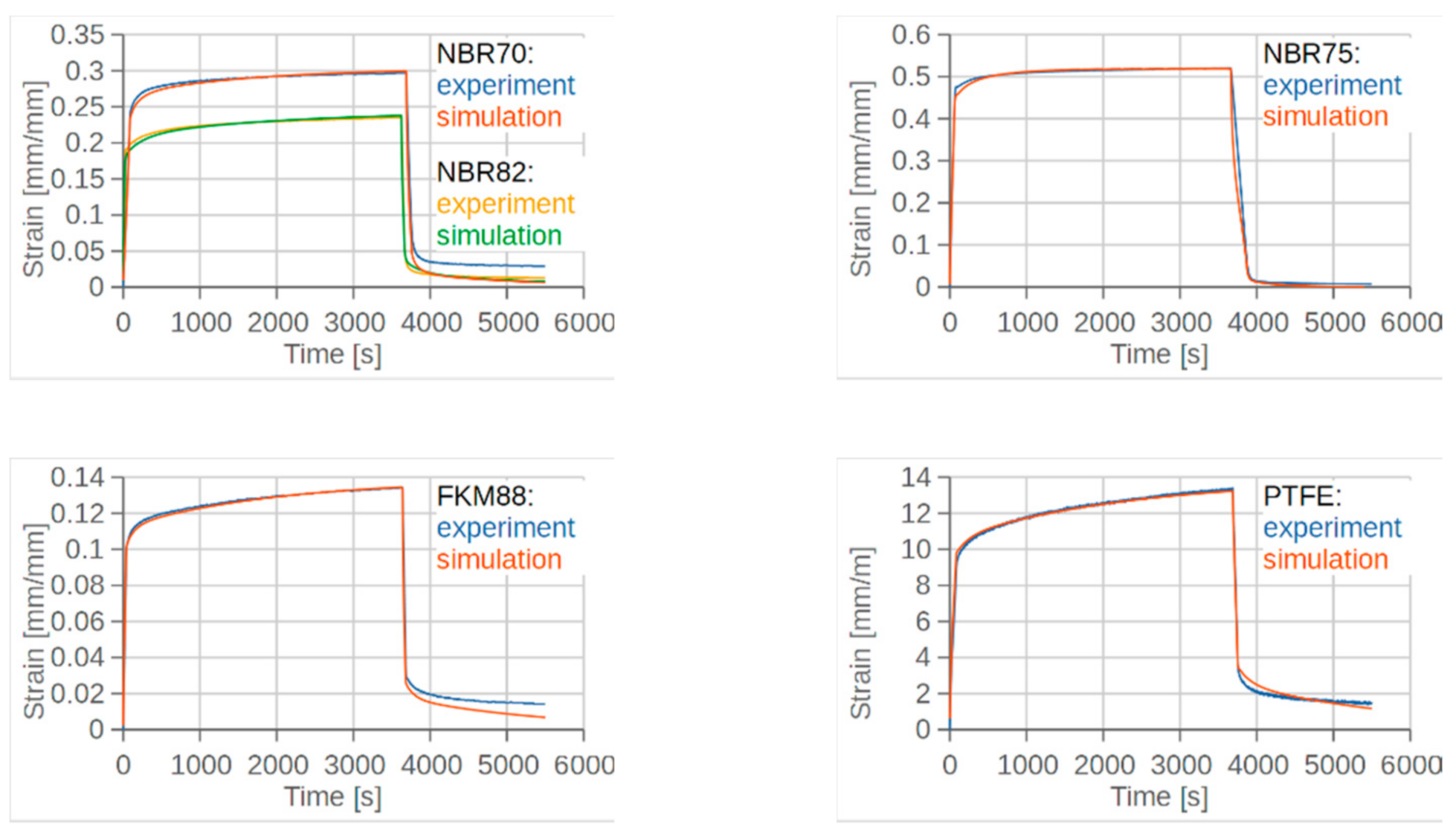
4.2. Material Modeling

The properties of all modeled materials in the FEM simulation are shown in Table 1. As already mentioned above, all counter parts of the seals, namely the rod, the housing, the piston, the floating piston and the tube could be modeled infinitely stiff since no significant deformations are expected for them. Given that FEM simulations with penetration-based contact detection converge better if some stiffness is set, in this research all of these parts are treated as a high-stiffness structural steel. The material’s density, which is equally required by the FEM solver, is also kept on the standard structural steel model value. The densities of the seal materials were determined by the use of a hydrostatic scale.
To appropriately model the characteristic stress–strain behavior of the seal materials within the FEM simulation, partly non-linear properties like stiffness, lateral contraction, viscoelasticity and viscoplasticity have to be considered. The material characterization was performed in constant stress tests on a tensile tester, as proposed in [19]. Such a test procedure is defined as a strain record under constant stress over a given period of time (in this research 1 h), and a subsequent strain record at zero stress (in this research 30 min) to characterize the back-deformation of the probe. The respective stress level per material probe was defined as it typically occurs during the shock absorber assembly.
Three different approaches have been investigated to model the non-linear material behavior during this research: the Prony shear relaxation model, the modified time hardening (MTH) model and the Bergström–Boyce model. It turned out that the Prony model as the simplest of these three is still sufficiently equipped to appropriately describe the seal’s materials. It adds linear viscoelastic behavior to a base elastic material model. Here, the base elastic material models are determined by the material’s initial shear modulus G 0 and density ρ , where the initial shear modulus G 0 is composed of the initial Young’s modulus E 0 and the Poisson’s ratio ν as follows:
G 0 = E 0 2 1 + ν
For elastomers and plastomers under a load far from their breaking load as they appear in this research, almost incompressible behavior can be assumed, which leads to the determination of constantly ν = 0.49 for all seal materials [19]. The viscoelastic behavior is subsequently modeled with a Prony series as a time-dependent decreasing shear modulus with the following form:
G t = G 0 G G 0 + i = 1 k G α i G e t τ i G
where t is the time, G t is the time dependent shear modulus, and G 0 and G are the initial shear modulus at t = 0 and the equilibrium shear modulus at t = . The qualitative shape of the relaxation curve is determined by the relative moduli α i G and the relaxation time τ i G [20]. The values presented in Table 1 are determined by curve fitting the aforementioned constant stress records.
A comparison of the material models with the parameters from Table 1 via constant stress FEM simulations versus the real test data is presented in Figure 5. As shown there, the simulation curves match the measured curves with higher than sufficient accuracy for the time period where the probe is loaded with constant stress (t < 3600 s). When the probes are unloaded, the quality of the match is mainly dependent on the amount of plastic deformation experienced by the real probe. Since the Prony model is only capable of modeling linear viscoelasticity, the plastic deformation experienced by the real probes while held under constant stress is recognized as viscoelastic in the curve-fitting process. The Prony shear relaxation model proved, therefore, it was suitable for the simulations performed in the context of this research.

4.3. Contact Modeling

As shown in Figure 2, a friction model is applied in the contact zone of the FEM simulation. To allow for that, an appropriate contact formulation and detection has to be implemented. The contact setup choices in this simulation are:
  • Augmented Lagrange contact formulation, a penetration-based contact definition, which provides decreased penetration and sensitivity to the contact normal stiffness compared to other penetration-based contact models.
  • On-Gauss-point contact detection, detecting a contact as soon as a contact surface’s Gauss point (i.e., one integration point of an element) penetrates the target surface.
  • 3D volumeless contact elements following the shape of the underlying 3D element and using an internal two-dimensional coordinate system to appropriately determine sliding distance, sliding direction and spatial contact stress distribution, as is generated by the friction model [20].
  • Standard Coulomb friction with μ = 0.4 on all rod guide assembly contacts which are expected to show no significant sliding, which is arbitrary, but within a reasonable range and found to be suitable to stabilize the setup by preventing flicking and gross sliding among these contacts.
  • Bonded contact definition for the piston band/piston contact, which is realistic due to the manufacturing process.
  • Standard Coulomb friction with μ = 0.4 between O-ring and floating piston to achieve reliable solution stabilization on this friction point. Since the pre-sliding displacement behavior implemented in dynamic friction models shows near-zero force response to very small displacements, the O-ring position in the floating piston’s groove is very unstable and, therefore, highly uncertain. This instability is increased by the use of a steady-state solver, where all time-dependent terms preventing motion damping due to the neglect of inertia are neglected, which is necessary to achieve suitable simulation time.

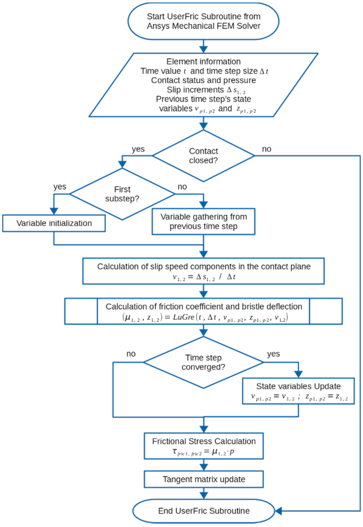
4.4. Friction Modeling

The choice of the dynamic friction model to be applied to the FEM simulation’s contact zone fell on the LuGre model [12,21]. The LuGre model presents the easiest handling and lowest parameterization requirements, whereas the aforementioned EP and Leuven/GMS approaches have the capability to model more friction effects, and provide thus more realistic behavior under certain circumstances. However, the distinguishing capabilities of the EP and Leuven/GMS models versus the LuGre model are not relevant among the boundary conditions of this research: First, the friction behavior of the damper is always a force response to a displacement actuation. Since this implies an always known and defined displacement, the LuGre model’s drifting behavior as a consequence of fluctuating force actuation never occurs [4,21,22,23,24]. The lack of appropriate non-local memory modeling within the LuGre model is also uncritical, since the intended actuation procedures do not contain sequences where the displacement direction is changed within the pre-sliding hysteresis without passing the zero-displacement (and thus also without passing the zero elastic bristle deflection state, too). The additional advantage of more realistic modeling of the pre-sliding regime of the GMS model [15,25] as well as of the Leuven model with the Maxwell slip approach [14,26] is also not needed in the above introduced approach: the better resolution of the pre-sliding regime in the GMS and Leuven models comes from the modeling of multiple bristles via Maxwell elements, which is also obtained within the presented approach. This is implemented by repeatedly calling the LuGre model in multiple FEM contact elements, taking into account changing contact geometry due to body deformations, material properties, displacement actuation or tangential stress due to the friction model itself.
The LuGre model as it is implemented in the proposed approach calculates friction as a linear combination of the three friction force contributors elastic bristle deflection, bristle damping and fluid damping:
F f r i c = σ 0 z + σ 1 z ˙ + σ 2 v
with z representing the average bristle deflection, σ 0 as bristle stiffness, σ 1 as bristle damping coefficient and σ 2 as speed-dependency describing viscosity coefficient. The dynamic average bristle deflection is modeled as:
d z d t = z ˙ = v σ 0 v g v z
where the speed-dependent function g v describes the gross sliding friction behavior through the Stribeck formulation:
g v = F C + F S F C e v / v S α
with F C as the Coulomb friction force, F S as the stiction force, v S the Stribeck velocity and α the Stribeck coefficient, which is usually kept constant at α = 2 to represent a Gaussian decay behavior [9].
The application of the LuGre model to each contact element generated between each seal and counterpart in the FEM simulation is performed through the USERFRIC interface provided by Ansys Mechanical, which enables to apply self-written friction models to detected contacts. The preferred programming languages for this task is Fortran and the closely Fortran-related Ansys Parametric Design Language (APDL), because the core FEM solver code of Ansys Mechanical is also written in Fortran. The overall implementation of the LuGre model is separated into two subroutines developed within this research. The first, namely the userfric subroutine, acts as an interface between the FEM setup and the actual friction model. The program flow chart of this userfric subroutine is depicted in Figure 6.
This subroutine hands over information from the FE solver that is required to solve the friction model, e.g., the current time step size and parameters which describe the contact status like contact pressure and slip increments per direction. It also initializes or gathers stored data from the previous FEM time step, namely the previous slip increments and the bristle deflection. Subsequently to the initialization and gathering, the current motion state is determined by the time-derivative of the slip increments in both directions of the contact element. With this data, the friction model is well defined and it is now called once per direction of the contact element. Separating the properties describing the element motion like slip increment and sliding speed is necessary, since the cell orientation as well as the sliding direction is usually unknown and can also change during the simulation progress. If the FEM solver converges on a solution for the current time step, the state variables z and v are updated. If the time step does not converge, the solver usually tries a bisection, which means a solution attempt with smaller time step size. For this case, the previous state variables are preserved to ensure appropriate initial conditions for the new time step. Subsequently, the frictional stress is calculated for the contact element, resulting in the determination of the slip distance and direction and the stored elastic energy of the contact element. Afterwards, the tangent matrix is updated and with that the friction contribution to the overall stress and deformation properties of the FEM setup is applied.
The second of the aforementioned subroutines is the LuGre subroutine, which contains the dynamic friction model itself. The corresponding program flow chart is depicted in Figure 7. The LuGre subroutine starts with parameter initialization or gathering from the previous time step handed over by the userfric subroutine. The determination of the respective single friction point parameter sets is described in Appendix A. These LuGre parameters are either hard coded to the subroutine or defined as a user input in Ansys Mechanical and handed over to the LuGre subroutine as a user-defined material property (see [20]). Next, it is determined whether the FEM simulation is still in the mounting phase, where all related contacts are defined as frictionless, since this leads to a faster solution process. If the FEM simulation is in the friction recording phase, the LuGre differential equation is solved numerically by a fourth order Runge Kutta algorithm. This integration algorithm uses a time step size which is 10 times smaller than the current FEM time step size. This linking of the Runge Kutta time step size and FEM time step size is very useful, since both the FEM setup and the friction algorithm require smaller time step sizes when the model becomes highly non-linear (e.g., when closing contacts or changing motion directions), and allow for larger time step sizes when the simulation does not experience major changes (e.g., at constant motion). The chosen factor 10 proved to be a good compromise of numerical stability versus calculation time.
Since the output of the LuGre model is a friction force, which is so far not influenced by the contact normal force within the implementation introduced above, the friction force F R within the LuGre subroutine is converted to the friction coefficient μ by the application of the additional parameter Ω :
μ = F R Ω
This parameter Ω represents the inverse normal force sensitivity of the friction contact and has the unit Newton to fulfill the convention of a friction coefficient with the unit [1]. It has to be tuned to an appropriate value subsequent to the FEM simulation, where Ω = 100 proved to be a good starting value. As a result of the introduction of Ω , the friction coefficient μ can be used for the tangential stress determination in the FEM setup as described above.
Both the LuGre and the userfric subroutine have been verified in FEM test cases which show very simple geometry (one-element block/plate pairings). Consequently, the related LuGre equations could be solved in Matlab, which enables for direct friction result comparison.

4.5. FEM Friction Simulation

Three phases determine the friction simulation sequence:
  • Mounting phase:
    Arrangement of all bodies and application of all boundary conditions to a state that resembles a newly constructed shock absorber, just recently mounted and pressurized.
    Resolving of the contact definitions of all corresponding damper parts in order to replace the initial penetration of the seals and counterparts (see Figure 4).
    Static pressure application to the parts which face a significant pressure drop in reality, namely the oil seal and the static seal. This is crucial since the correct contact pressure of the oil seal against the rod is additionally determined by the static pressure in the damper, whereas the contact pressure of the other seal contacts (scraper, piston band, floating piston’s O-ring) is only determined by the seal’s deformation due to the contact definition.
  • Relaxation phase: This represents the period of time that is needed by the viscoelastic material model to reach a nearly steady state. After this phase a state is reached, which resembles the initial state of the friction recording phase of the single friction point measurements from part 2 of this study. Analysis of the simulation of the relaxation phase showed that a relaxation time of half an hour is sufficient to achieve this desired steady state, which is easily verifiable, given that the ongoing relaxation during the following friction recording phase would result in a decreasing contact pressure, which would result in constantly decreasing friction during actuation.
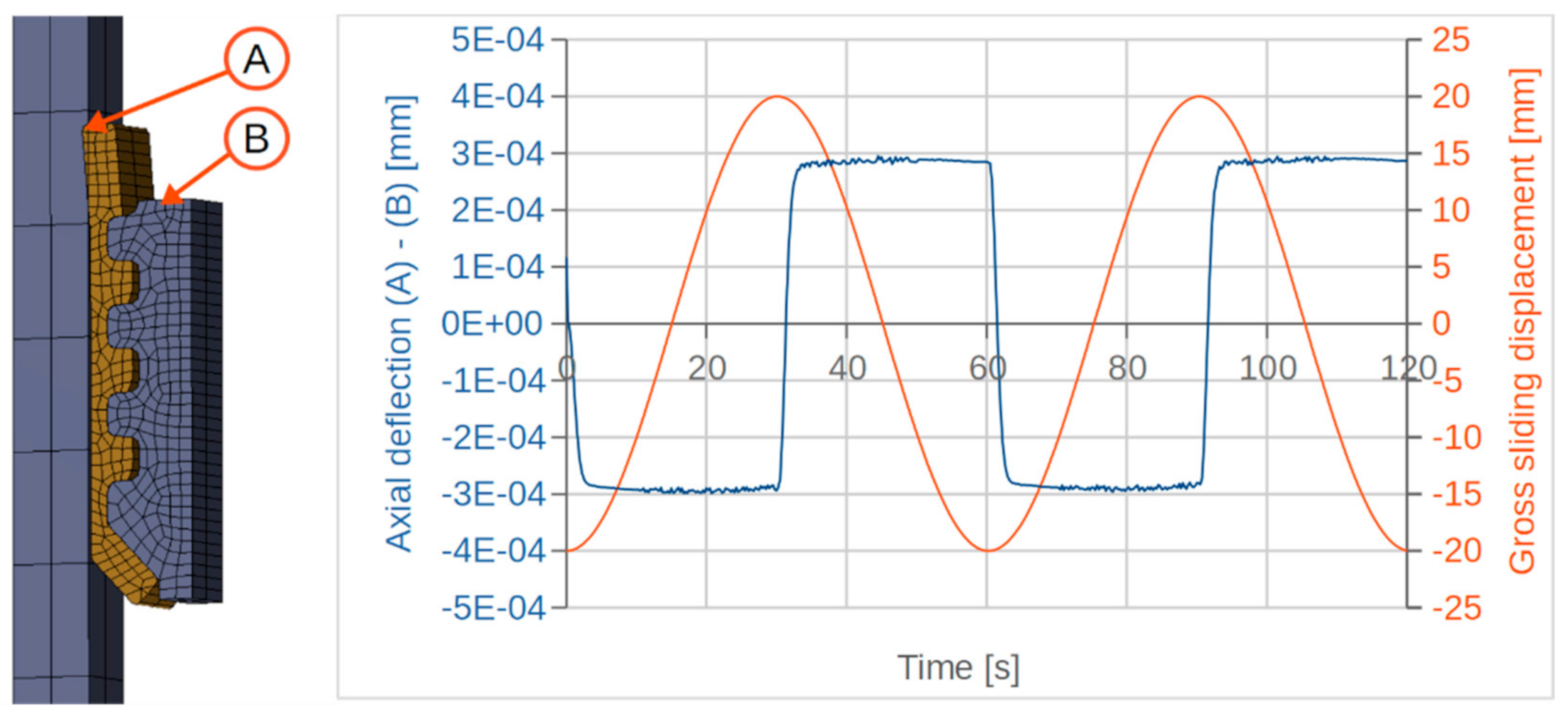
  • Friction recording phase: Here, the actuation itself is applied as a time-dependent displacement boundary condition at the piston, the rod and the floating piston. It follows the reference friction recording sequence presented in part 2 of this study, a sine function with a period of 60 s and an amplitude of 20 mm, which corresponds to a maximum speed of about 2.1 mm/s. The related displacement amplitude for the floating piston/tube friction point is 1.85 mm according to the aforementioned hydraulic transmission, which corresponds to a maximum speed of about 0.2 mm/s.
The equation solver type used for all simulations is configured as follows:
  • Use of the implicit Sparse Direct Equation Solver of Ansys Mechanical APDL;
  • Use of both large deflections and enforced use of line search algorithms to achieve stable convergence as well as reliable results;
  • Use of a fully asymmetric Newton-Raphson method for the determination of the minimum of the potential energy of the FEM setup, since the whole setup is significantly nonlinear due to the contact definition, the friction model, the material data and the large deflections.
Because of the purposeful simplifications of the simulation geometry, which leads to a low overall element count, the simulation time for a full simulation run on common work station hardware is only between 20 min (piston/tube) and 75 min (rod guide assembly/rod) and, therefore, still reasonable for the intended use in daily engineering.

5. Results

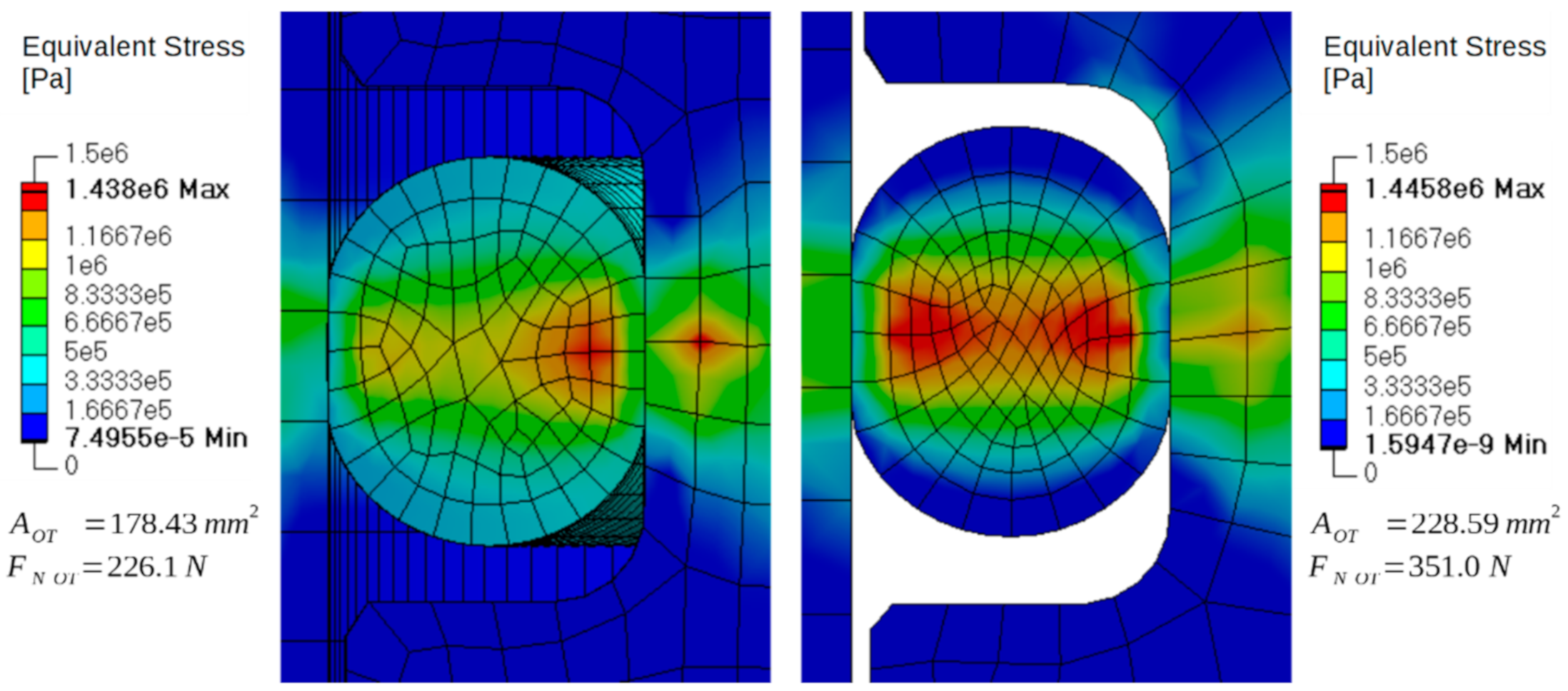
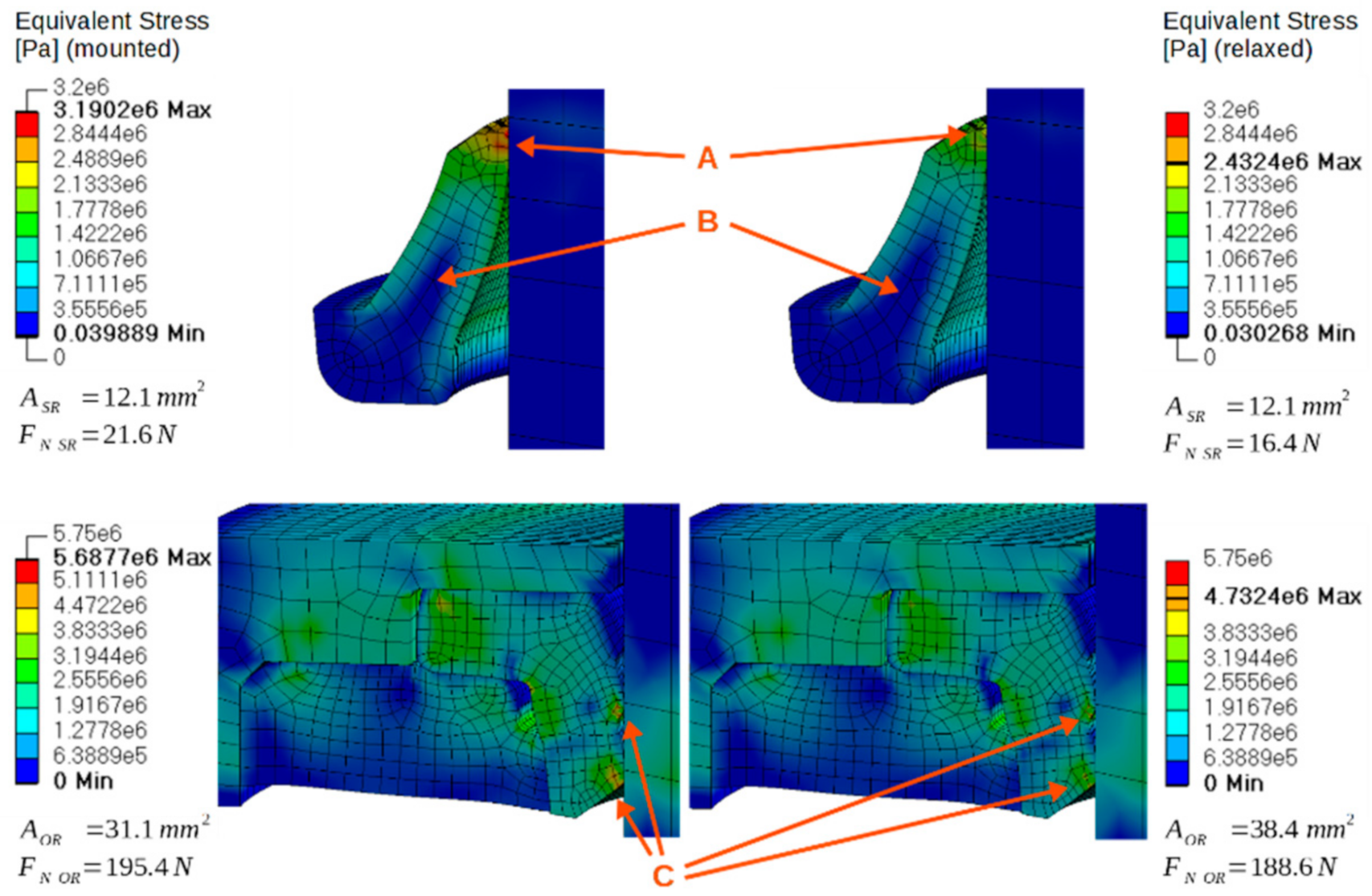
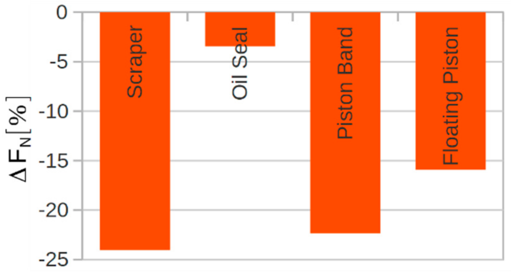
5.1. FEM Results Overview

The analysis of the stress distribution, the contact resolution, and solid body motion and deformation acts as a plausibility check for the overall setup and provides insights into the general behavior of the respective single friction point under the defined loads, apart from the friction behavior. To keep this section brief, the rod guide assembly rod friction point as the most complex one is presented here, exemplarily for all single friction points. Its equivalent stress distribution is shown in Figure 8, where the left panel shows the equivalent stress distribution just after mounting, and the right panel shows the equivalent stress distribution after an additional 30 min of standstill. This state of the right panel represents the state of the simulation setup just prior to the friction recording sequence, where the setup is mounted, pressurized to operating pressure, and at least half an hour has passed at standstill so as to achieve proper material relaxation as explained above.
The related overall equivalent stress decrease of the scraper/rod pairing is best visible near the contact zone (A) and by the enlarged blue area within the scraper’s body (B). The scraper/rod contact shows no unexpected behavior, since no further parts or boundary conditions are involved. The contact resolution shows good convergence represented by barely visible body penetration, and the qualitative equivalent stress distribution is reasonable considering the boundary conditions and the deformation distribution. The shown quantitative range of equivalent stress and the resulting contact normal force are reasonable due to the material stiffness and deformation. Because of the simple setup without further influences on the bodies, the contact area change resulting from the material relaxation phase is insignificant (+0.05%), while the change of the contact normal force is significant (−24.0%) but reasonable following the material formulation.
The oil seal/rod contact behavior in Figure 8 is significantly different from that of all other seal/counterpart contacts because of the additional impact from the static pressure-loaded static seal. This part is transmitting the damper’s static operating pressure to the oil seal/rod contact due to its geometric and material properties. The therefore increased oil seal/rod contact pressure ensures the tightness of the oil seal, especially in high-speed scenarios. The consequence of the combination of oil seal, static seal and static pressure is a significantly increased average stress level in both the oil seal and the static seal, as compared to the scraper. This equivalent stress level is decreasing during the relaxation phase, as expected, which is best visible at the contact zones (C), but as well through the more pronounced blue shading within the less deformed parts of the seals. Simultaneously, the oil seal/rod contact area increases much more significantly than at the scraper/rod contact or at the piston band/tube contact (+23.4%). This increase is caused by the ongoing deformation of the relaxing static seal, leading to even further increased pressure on the oil seal. As a consequence, this influence of the static seal on the oil seal leads to an only slightly decreasing circumferential contact normal force in the oil seal/rod contact during the relaxation phase (−3.4%).
All resulting contact normal force changes of the seal/counterpart contacts during the material relaxation phase are plotted together in Figure 9. The contact normal force F N is directly influencing the friction force generated in the FEM contact by the friction model, as introduced above and is, therefore, a very important parameter with regard to the overall friction simulation behavior. However, it should not be investigated without consideration of the contact geometry and contact discretization, since both influence the derived contact area, as discussed in the simulation setup. Notwithstanding these considerations, the qualitative F N change during the relaxation phase represents the qualitative change in expected friction generation, and is therefore worth investigating.
The general expectation for the development of F N during the relaxation phase is a significant decrease, as is experienced by the scraper/rod contact, the piston/tube contact and the floating piston/tube contact in Figure 9. However, in certain setups with additional influences through third bodies or external boundary conditions, a less significant contact normal force decrease or even a contact normal force increase during the relaxation phase is possible, as experienced by the oil seal/rod contact. Consequently, it is not clear if the circumferential contact normal force F N is increasing or decreasing, or if the amount of F N change is estimable with acceptable accuracy prior to a friction simulation, if viscoelastic material behavior occurs similar to the simulations setups presented here. This is why appropriate material modeling as introduced above is crucial for the accuracy of seal/counterpart friction simulations.

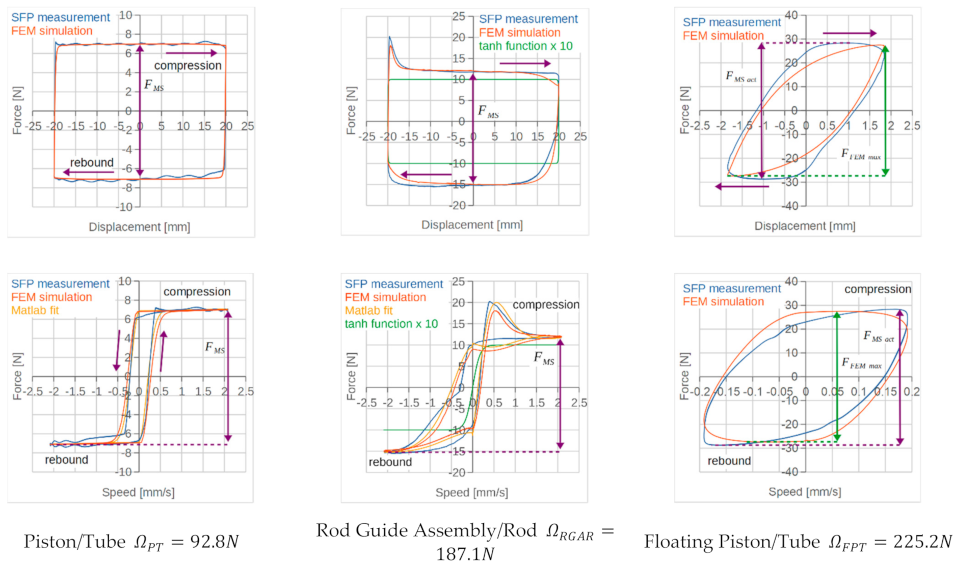
5.2. Analysis of the Simulated Friction Force Behavior

Figure 10 shows the friction simulation results of each single friction point, both as force-displacement graphs (top) and force-speed graphs (bottom) in comparison to the reference friction measurement results from the single friction point test rigs introduced in part 2 of this study. For comparison, the force-speed graph of the Matlab-optimized friction graph without the related FEM simulation (Matlab fit) is also depicted. The simulated friction forces are obtained from the FEM simulation as force reactions to the respective exciting displacement boundary conditions. Prior to these simulation results, the above-introduced inverse contact normal force sensitivity Ω is tuned for each single friction point to quantitatively match the midstroke friction force F M S of FEM simulation data and measurement data.
The arising differences between Ω P T ,   Ω R G A R and Ω F P T are resulting in differently high friction force generation per circumferential contact normal force of the respective seal. This behavior is reasonable, since hydrodynamic friction is usually less affected by increasing normal force than dry or mixed friction. The differences in Ω are, therefore, most probably caused by the different states of lubrication in the single friction points, given that the piston band/tube contact is facing damper oil from both sides, whereas the oil seal/rod friction point is only facing oil from the lower side, and the scraper/rod contact is experiencing lubrication only by leftover oil or additional grease on the rod. Similarly, Ω F P T is even higher than Ω R G A R , implying an overall even less lubricated state than in the rod guide assembly/rod friction point. This interpretation is reasonable as well, given that one side of the floating piston’s O-ring is only lubricated with almost non-existent leftover oil on the tube due to near zero leakage.
The qualitative shape of both the FEM force-displacement graph and the FEM force-speed graph with their SFP measurement counterparts is matching sufficiently well. The piston/tube friction point show almost perfect matching with only a slight widening of the pre-sliding hysteresis compared to both the measurement data and the Matlab fit in Figure 10. The width of the pre-sliding hysteresis is mainly determined by σ 0 and σ 1 from the LuGre model formulation. The reason for the slightly widened hysteresis is to be found in the deformation behavior of the seal lip in the FEM simulation due to the applied friction force. The seal lip acts as an additional spring-damper combination, which changes its deflection during speed changes and displacement reversals.
This deflection behavior is visualized in Figure 11 by the comparison of the displacement boundary condition (orange) applied to the piston and the axial distance (blue) between the end lip of the piston band (A) and the displacement application face of the piston (B) during the friction recording phase. As shown in Figure 11, the axial distance between (A) and (B) is decreased during rebound (the spring-damper combination is compressed) and is increased during stroke (the spring-damper combination is stretched). The amount of (A)–(B) distance change is dependent on the viscoelastic material data of the piston band, and on the friction force generated in the piston band/tube contact. The amount of friction in the piston band/tube contact is also dependent on the material data, given that the material data determines the contact normal force due to the lateral deformation of the seal. The piston band/tube friction is further dependent on the amount and rate of the displacement boundary condition of the piston, of the seal lip’s axial spring-damper deflection, the contact normal force sensitivity and the LuGre parameter set. As a consequence of the dependency on these various parameters, the individual contribution of the additional spring-damper combination behavior of the seal lip to the friction behavior can not be easily determined or corrected. The measurement data represents merely the friction force versus displacement and speed between the actuated piston and the tube. All occurring lip seal deflection, which contributes to the pre-sliding hysteresis of the recorded friction behavior, is already covered in the LuGre parameter set through the Matlab fit, and therefore covered twice in the overall FEM friction simulation model: The seal lip deflection occurring in the FEM simulation is added to the LuGre pre-sliding deflection in the contact zone. Since the additional spring and damper of the seal lip are linked in parallel to each other, but in series to the spring and damper modeling of the LuGre model, their contribution to the overall deformation and stress level results in a decrease of spring stiffness and damper rate. According to the LuGre modeling, this decrease of spring stiffness and damper rate can be understood as a decreasing σ 0 and σ 1 and, therefore, leads to an underestimation of tangential contact stiffness and tangential contact damping. Consequently, a widening of the pre-sliding hysteresis of the FEM simulation according to the SFP measurement data and the Matlab fit has to occur.
Despite these expected difficulties, the width difference of the pre-sliding hysteresis of the FEM model compared to the single friction point measurement in Figure 10 (left) is very small, which implies only a weak link between microscopic and macroscopic material behavior. This is crucial and has to be ensured for all friction points, because the presented simulation methodology strictly separates macroscopic material behavior as input parameters for the structural FEM setup, and microscopic material behavior as input parameters for the dynamic friction model. However, the influence of the macroscopic material behavior on the qualitative shape of the force-displacement and force-speed graphs should be considered when analyzing similar simulation results.
The qualitative deviations between the FEM simulation and the single friction points measurements of the rod guide assembly/rod friction point are a decreased height and width of the force overshoot after the motion direction turnaround from rebound to compression, a minimally shifted, but not width-altered pre-sliding hysteresis, and a slightly too-low force level of the FEM simulation over the whole decreasing-speed part from compression to rebound of the friction recording phase. The reason for these qualitative differences in friction behavior, is most likely the same reason as for the qualitative friction graph deviations at the piston/tube friction point as mentioned above: Since the seals respond with axial deformation to the friction force generated in the respective contact zones while stroking, additional spring and damper elements are added to the friction simulation system. These additional spring and damper elements consequently act as a reduction of the LuGre parameters σ 0 and σ 1 therefore cause the mentioned deviations. Nevertheless, the qualitative friction behavior of the rod guide assembly/rod friction point is described by the introduced friction modeling approach witch high accuracy.
The qualitative deviations between experiment and simulation at the floating piston/tube friction point are greater than for the other two friction points. This is to be expected, since different actuation sequences are used for the parameter estimation and the FEM friction simulation, as introduced in the simulation setup section. Consequently, this simulation acts as a validation of the transferability of both the LuGre parameter set and the inverse contact normal force sensitivity Ω . Since Ω influences the quantitative amount of friction, also quantitative differences between simulation and experiment occur for this single friction point in Figure 10 (right), which are, however, acceptably low (−3.9% for F F E M m a x ). The most probable reasons for the differences in qualitative friction behavior are therefore uncertainties from the parameter set transfer and influences from the very low actuation displacement amplitude, which is—according to the LuGre parameter set—never leaving the pre-sliding range. This is unique for all investigated friction points, and not the optimal application for the LuGre model. However, the qualitative deviations between the FEM simulation and the single friction point measurement are still sufficiently small. Together with the very low quantitative deviation it is, therefore, shown that the floating piston/tube friction point is described in its friction behavior with sufficient accuracy by the introduced friction modeling approach.

6. Conclusions

Automated driving dictates new requirements for ride quality comfort. Therefore, modeling and especially experimental evaluation of shock absorbers is essential. One of the key problems is the reproduction of the friction behavior from the reference measurements. In the presented study this representation is sufficiently accurate, as could be expected from the accuracy of the friction model parameterization. The friction simulation slightly underestimates contact stiffness and contact damping, which is model-immanent due to the imperfect separability of microscopic and macroscopic seal deformation behavior. The simulation of damper friction is possible with high qualitative and quantitative accuracy, while requiring a reasonably small amount of parameterization measurements, and remarkably low calculation time compared to the large number of considered friction-influencing parameters. The validation of this simulation approach and the transferability of the gathered friction model parameters to different geometry is presented in part 2 of this study. This opens a wide field for further optimization of automotive shock absorbers regarding friction in all design stages by studying the influence of the considered parameters in various simulations. Given that this methodology is not limited to the analysis of automotive shock absorbers, but should be applicable to most types of friction investigations of hydraulic seals, a wide field of further application and specific adaptation lies open and could be explored in future work.

Author Contributions

Supervision, K.A.; Everything else, L.H.; All authors have read and agreed to the published version of the manuscript.

Funding

The APC was funded by the Open Access Publication Fund of the Technische Universität Ilmenau.

Acknowledgments

We acknowledge support for the publication costs by the Open Access Publication Fund of the Technische Universität Ilmenau.

Conflicts of Interest

The authors declare no conflict of interest.

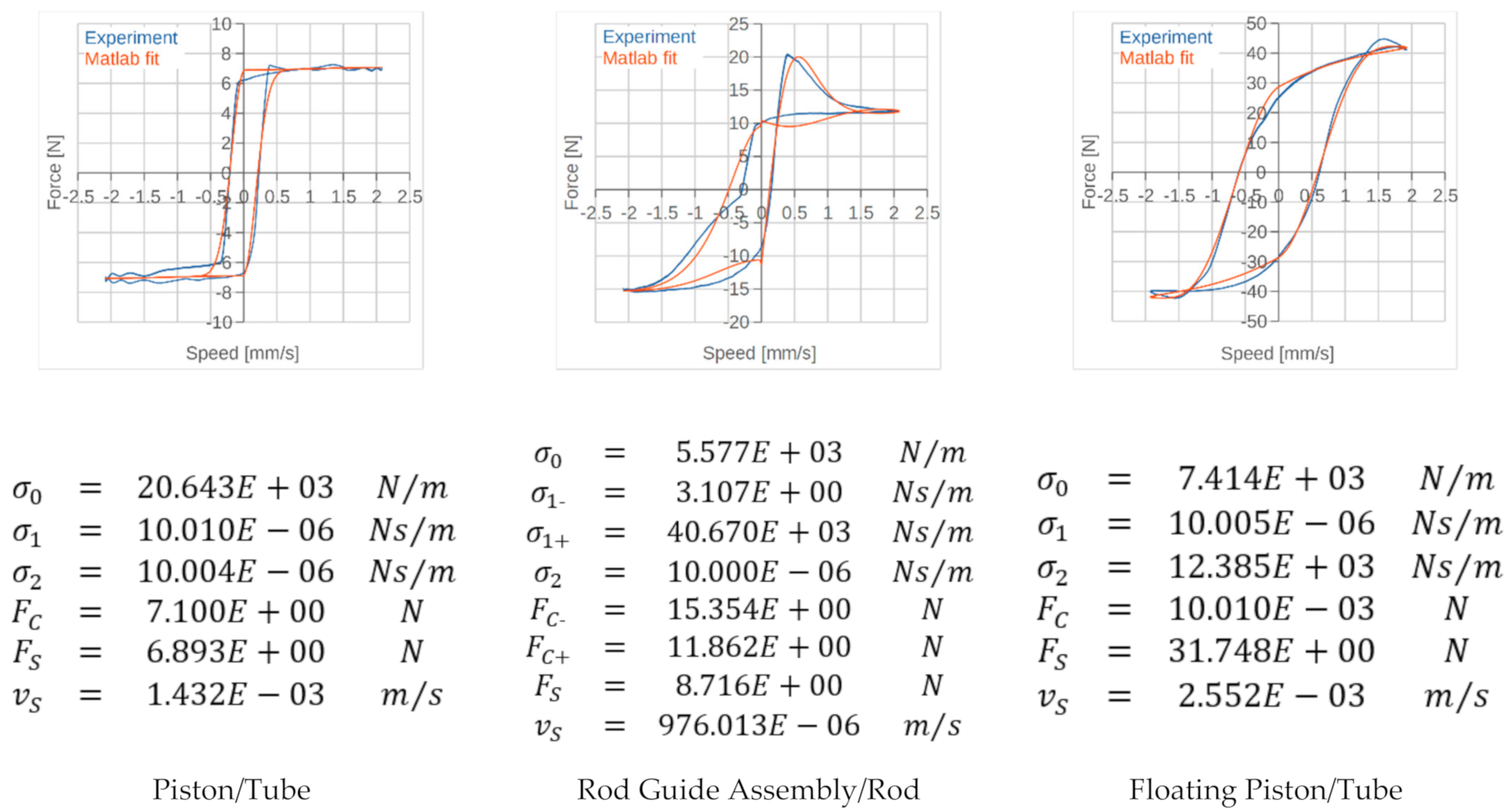
Appendix A. Friction Model Parameterization

The parameters determining the friction behavior of the LuGre model are σ 0 , σ 1 , σ 2 , F C , F S and v S (see Equations (4)–(6)). An efficient way of obtaining these parameters from reference single friction point measurements (see part 2 of this study) is performing optimizations, e.g., by use of the lsqcurvefit function within Matlab. All three single friction points are parameterized with one parameter set, respectively. This also applies to the rod guide assembly/rod friction point, even if it contains two actual friction points (see Figure 1), since efficiently measuring scraper/rod or oil seal/rod friction independently, but under realistic operating conditions, is virtually impossible. However, dependent on an appropriate initial guess, very well matching friction graphs are achieved as shown in Figure A1, which also presents the respective parameter sets for each single friction point.
Figure A1. Parameterization results for each single friction point, showing a sufficiently accurate match of the respective force-speed graphs.
Vehicles 03 00014 g0a1
Remarkable specifics of the parameterization concern the rod guide assembly/rod friction point and the floating piston/tube friction point. For the former, the significantly asymmetric force-speed behavior demands for a partly speed direction-dependent parameter set, where the respective parameters σ 1 + / and F C + / are blended near zero speed via a tanh function of the form:
σ 1 = σ 1 + + σ 1 2 + σ 1 + σ 1 + + σ 1 2 t a n h v a m p
with a m p determining the slope of the tanh function near zero speed. Since this blending has also to be implemented to the friction model applied to the FEM simulation’s contact zones, a m p has to be chosen high (about 10e6) during the parameterization process, but smaller (about 3000) during the FEM simulation to ensure a sufficient compromise of smooth blending and accurate near-zero speed friction description. For the latter, the floating piston/tube friction point, the much smaller (about 9.3%) sliding distance compared to the other friction points during the reference friction recording cycle leads to a slightly differing parameterization approach. This smaller sliding distance is caused by the indirect actuation of the floating piston only caused by the volume compensation of the entering rod (see Figure 1). Since some of the LuGre parameters are mainly determining the high-speed friction behavior (e.g., σ 2 and v S ), the aforementioned small sliding distance measurement data is no sufficient basis for the fitting of these parameters. Instead, a ten times larger friction recording sequence was used for the parameterization of the floating piston/tube friction point, which brought well matching simulation results even for smaller sliding distances, as presented in the results section of this article.

References

  1. Shyrokau, B.; Wang, D.; Savitski, D.; Hoepping, K.; Ivanov, V. Vehicle Motion Control with Subsystem Prioritization. Int. J. Mechatron. 2015, 30, 297–315. [Google Scholar] [CrossRef]
  2. Alfonso, J.; Rodriguez, J.M.; Salazar, J.C.; Orús, J.; Schreiber, V.; Ivanov, V.; Augsburg, K.; Castellanos, J.A. Distributed Simulation and Testing for the Design of a Smart Suspension (12-03-02-0011). SAE Int. J. Connect. Autom. Veh. 2020, 3, 129–138. [Google Scholar]
  3. Heipl, O.P. Experimentelle und numerische Modellbildung zur Bestimmung der Reibkraft translatorischer Dichtungen. Ph.D. Thesis, Fakultät für Maschinenwesen, RWTH Aachen, Aachen, Germany, 2013. [Google Scholar]
  4. Mofidi, M. Tribology of elastomeric seal materials. Ph.D. Thesis, Department of Applied Physics and Mechanical Engineering, Division of Machine Elements, Luleå University of Technology, Luleå, Sweden, 2009. [Google Scholar]
  5. Wangenheim, M. Untersuchungen zu Reibmechanismen an Pneumatikdichtungen. Ph.D. Thesis, Institut für Dynamik und Schwingungen, Gottfried Wilhelm Leibniz Universität Hannover, Hannover, Germany, 2012. [Google Scholar]
  6. Al-Bender, F. Fundamentals of Friction Modeling; Department of Mechanical Engineering, Division PMA Katholieke Universiteit Leuven: Leuven, Belgium, 2010. [Google Scholar]
  7. Wojewoda, J.; Stefanski, A.; Wiercigroch, M.; Kapitaniak, T. Hysteretic effects of dry friction: Modelling and experimental studies. In Philosophical Transactions of the Royal Society A | Mathematical, Physical & Engineering Sciences; Division of Dynamics, Technical University of Łódź: Łódź, Poland; Centre for Applied Dynamics Research, School of Engineering, University of Aberdeen, King’s College Aberdeen: Aberdeen, UK, 2008. [Google Scholar]
  8. Armstrong-Hélouvry, B.; Dupont, P.; de Wit, C.C. A Survey of Models, Analysis Tools and Compensation Methods for the Control of Machines with Friction; Elsevier Science Ltd.; University of Wisconsin: Milwaukee, WI, USA, 1994. [Google Scholar]
  9. Rudermann, M. Zur Modellierung und Kompensation dynamischer Reibung in Aktuatorsystemen. Ph.D. Thesis, Fakultät für Elektrotechnik und Informationstechnik, Lehrstuhl für Regelungssystemtechnik, Technische Universität Dortmund, Dortmund, Germany, 2012. [Google Scholar]
  10. Dahl, P.R. A Solid Friction Model; The Aerospace Corporation: El Segundo, CA, USA, 1968. [Google Scholar]
  11. de Wit, C.C.; Olsson, H.; Åström, K.J.; Lischinsky, P. A New Model for Control of Systems with Friction. IEEE Trans. Autom. Control 1995, 40, 419–425. [Google Scholar] [CrossRef] [Green Version]
  12. Dupont, P.; Armstrong, B.; Hayward, V. Elasto-Plastic Friction Model: Contact Compliance and Stiction. In Proceedings of the American Control Conference, Chicago, IL, USA, 28–30 June 2000; Aerospace & Mechanical Engineering, Boston University: Boston, MA, USA, 2002. [Google Scholar]
  13. Shyrokau, B.; Wang, D.; Augsburg, K.; Ivanov, V. Vehicle Dynamics with Brake Hysteresis. Imeche Part. D J. Automob. Eng. 2013, 227, 139–150. [Google Scholar] [CrossRef] [Green Version]
  14. Swevers, J.; Al-Bender, F.; Ganseman, C.G.; Prajogo, T. An Integrated Friction Model Structure with Improved Presliding Behavior for Accurate Friction Compensation. IEEE Trans. Autom. Control 2000, 45, 675–686. [Google Scholar] [CrossRef]
  15. Lampaert, V.; Al-Bender, F.; Swevers, J. A generalized Maxwell-slip friction model appropriate for control purposes. In Proceedings of the IEEE International Workshop on Workload Characterization (IEEE Cat. No.03EX775), St. Petersburg, Russia, 20–22 August 2003; Department of Mechanical Engineering, Katholieke Universiteit Leuven: Leuven, Belgium, 2003. [Google Scholar]
  16. Blok, H. Inverse problems in hydrodynamic lubrication and design directives for lubricated flexible surfaces. In Proceedings of the International Symposium on Lubrication and Wear, Houston, TX, USA, 1 January 1963. [Google Scholar]
  17. van Leeuwen, H.J.; Schouten, M.J.W. Die Elastohydrodynamik: Geschichte und Neuentwicklungen. In VDI Berichte Nr. 1207; Eindhoven University of Technology: Eindhoven, The Netherlands, 1995. [Google Scholar]
  18. Kaiser, F. Ein Simulationsmodell zur Analyse des Schmierfilms von Stangendichtungen. In Dissertation; Lehrstuhl für Maschinenelemente und Getriebetechnik, TU Kaiserslautern: Kaiserslautern, Germany, 2015. [Google Scholar]
  19. Frick, A.; Stern, C. Einführung in die Kunststoffprüfung—Prüfmethoden und Anwendungen; Carl Hanser Verlag: München, Germany, 2017. [Google Scholar]
  20. ANSYS, Inc. ANSYS Mechanical APDL Theory Reference Version 2020 R1; ANSYS, Inc.: Canonsburg, PA, USA, 2020. [Google Scholar]
  21. Åström, K.J.; de Wit, C.C. Revisiting the LuGre friction model. IEEE Control Syst. Mag. 2008, 100–114. [Google Scholar]
  22. van Geffen, V. A Study of Friction Models and Friction Compensation; Technische Universiteit Eindhoven, Department Mechanical Engineering, Dynamics and Control Technology Group: Eindhoven, The Netherlands, 2009. [Google Scholar]
  23. Al-Bender, F.; Swevers, J. Characterization of Friction Force Dynamics. IEEE Control. Syst. Mag. 2008, 28, 64–81. [Google Scholar]
  24. Ruderman, M.; Bertram, T. Modified Maxwell-Slip model of presliding friction. In Proceedings of the 18th IFAC World Congress, Milan, Italy, 28 August–2 September 2011. [Google Scholar]
  25. Al-Bender, F.; Lampaert, V.; Swevers, J. A novel generic model at asperity level for dry friction force dynamics. In Tribology Letters; Department of Mechanical Engineering, Katholieke Universiteit Leuven: Leuven, Belgium, 2003; Volume 16. [Google Scholar]
  26. Lampaert, V.; Swevers, J.; Al-Bender, F. Modification of the Leuven Integrated Friction Model Structure. IEEE Trans. Autom. Control 2002, 47, 683–687. [Google Scholar] [CrossRef] [Green Version]
Figure 1. Reference damper overview with details of the single friction points. (A) Rod guide assembly/rod; (B) piston/tube; (C) floating piston/tube.
Vehicles 03 00014 g001
Figure 2. Solution approach overview; three main parameter groups are included in the simulation either directly or indirectly via experimental parameterization.
Vehicles 03 00014 g002
Figure 3. Comparison of the equivalent stress distribution in a rotational symmetric FEM setup (left) and a flat 2.5 D FEM setup (right) with the resulting contact area A O T and circumferential O-ring/tube contact normal force F N O T .
Vehicles 03 00014 g003
Figure 4. Geometry abstraction and mesh (undeformed) for the FEM simulation; left: 4° wedge of the rod guide assembly/rod friction point; center: 4° wedge of the piston/tube friction point; right: 4° wedge of the floating piston/tube friction point.
Vehicles 03 00014 g004
Figure 5. Comparison of constant stress test results versus constant stress FEM simulation for each seal material modeled with the Prony shear relaxation material model.
Vehicles 03 00014 g005
Figure 6. Program flow chart of the userfric subroutine.
Vehicles 03 00014 g006
Figure 7. Program flow chart of the LuGre subroutine.
Vehicles 03 00014 g007
Figure 8. Comparison of the equivalent stress distribution of the rod guide assembly/rod FEM setup, divided into the scraper/rod contact (top) and the oil seal/rod contact (bottom) before (left) and after (right) material relaxation time, with the resulting contact areas A S R and A OR and the circumferential scraper/rod and oil seal/rod contact normal forces F N S R and F N OR .
Vehicles 03 00014 g008
Figure 9. Contact normal force change (in percentage) during the material relaxation phase, depicted for each seal/counterpart FEM contact.
Vehicles 03 00014 g009
Figure 10. Comparison of the FEM simulations and the single friction point measurements of the friction behavior of all three friction points.
Vehicles 03 00014 g010
Figure 11. Left panel: FEM model of the piston/tube friction point including the end lip of the piston band (A) and the displacement application face of the piston (B). Right panel: comparison of the displacement boundary condition applied to the piston (orange) and the distance between (A) and (B) (blue) during the friction recording phase.
Vehicles 03 00014 g011
Table 1. Material model data for the FEM simulation, containing density, stiffness, lateral stiffness and the Prony model parameters.
MaterialDensity ρ k g / m 3 Young’s Modulus E ; E 0 M P a Poisson’s Ratio ν 1 Relative Moduli α i G 1 Relaxation Time τ i G s
NBR70 (O-Ring)12147.780.49(1)0.0707(1)1448.6
(2)0.0735(2)130.2
(3)0.0395(3)8.8
NBR75 (Static Seal)12758.240.49(1)0.0339(1)470.2
(2)0.0148(2)161.3
(3)0.0689(3)11.7
NBR82 (Scraper)144815.870.49(1)0.0787(1)1860.2
(2)0.0827(2)216.8
(3)0.1321(3)8.7
FKM88 (Oil Seal)201026.470.49(1)0.1336(1)1655.2
(2)0.0834(2)103.8
(3)0.0694(3)7.2
PTFE (Piston Band)2300680.970.49(1)0.1167(1)149.0
(2)0.2027(2)1748.9
Steel (All Others)7850200,0000.3--
Publisher’s Note: MDPI stays neutral with regard to jurisdictional claims in published maps and institutional affiliations.

