
A Survey of Path Planning Algorithms for Mobile Robots


1
Department of Electrical and Computer Engineering, Michigan State University, East Lansing, MI 48824, USA
2
Halla Mechatronics, 3933 Monitor Rd, Bay City, MI 48706, USA
3
Department of Computer Science and Engineering, Michigan State University, East Lansing, MI 48824, USA
*
Author to whom correspondence should be addressed.
Vehicles 2021, 3(3), 448-468; https://0-doi-org.brum.beds.ac.uk/10.3390/vehicles3030027
Submission received: 27 May 2021
/
Revised: 19 July 2021
/
Accepted: 25 July 2021
/
Published: 4 August 2021
(This article belongs to the Special Issue Electrified Intelligent Transportation Systems)
Abstract
:Path planning algorithms are used by mobile robots, unmanned aerial vehicles, and autonomous cars in order to identify safe, efficient, collision-free, and least-cost travel paths from an origin to a destination. Choosing an appropriate path planning algorithm helps to ensure safe and effective point-to-point navigation, and the optimal algorithm depends on the robot geometry as well as the computing constraints, including static/holonomic and dynamic/non-holonomically-constrained systems, and requires a comprehensive understanding of contemporary solutions. The goal of this paper is to help novice practitioners gain an awareness of the classes of path planning algorithms used today and to understand their potential use cases—particularly within automated or unmanned systems. To that end, we provide broad, rather than deep, coverage of key and foundational algorithms, with popular algorithms and variants considered in the context of different robotic systems. The definitions, summaries, and comparisons are relevant to novice robotics engineers and embedded system developers seeking a primer of available algorithms.
Autonomous Vehicles (AVs) have the potential to dramatically reduce the contribution of human driver error and negligence as the cause of vehicle collisions. These AVs must move from point A to point B safely and efficiently with respect to time, distance, energy, and other factors. Path planning is key in determining and evaluating plausible trajectories in support of these goals.
While performing navigational tasks, robotic systems, such as AVs, make use of capabilities that involve modeling the environment and localizing the system’s position within the environment, controlling motion, detecting and avoiding obstacles, and moving within dynamic contexts ranging from simple to highly complicated environments. The four general problems of navigation are perception, localization, motion control, and path planning [1,2,3].
Among these areas, it may be argued that path planning is the most important for navigation processes. Path planning is the determination of a collision-free path in a given environment, which may often be cluttered in a real world situation [4]. To best take advantage of these capabilities while accomplishing the system’s design and use objectives, an appropriate path planning technique must be identified and implemented. Often, the best-performing technique will vary with the system type and operating environment.
As mobile AVs have proliferated and increasingly require path planning or path finding, these capabilities have become a recent area of focus in the field of autonomous control. Since mobile robots are used in a range of applications, researchers have developed methods for effectively fitting their requirements to overcome some of the significant challenges faced while implementing fully or partially autonomous navigation in cluttered environments.
In order to simplify the path planning problem and ensure that the robot runs/moves smoothly while avoiding obstacles in a cluttered environment, the configuration space must be matched with the algorithm being used. Multiple path planning and path finding algorithms exist with varied applicability determined by the system’s kinematics, the environment’s dynamics, robotic computation capabilities, and sensor- and other-sourced information availability. Algorithm performance and complexity trade-offs also depend on the use case.
For a novice practitioner, selecting just one approach is daunting—particularly for those individuals without a background in controls. Yet, as AVs become increasingly widespread, engineers are forced into such roles without adequate training. This document aims to provide a summary of commonly used foundational techniques for path planning suitable for individuals with limited expertise in controls and seeking to identify areas of exploration in support of new AV functionality.
We consider the applicability of algorithms in static and dynamic environmental contexts and review common path planning algorithms used in autonomous vehicles and robotics to serve as a primer for novice practitioners in the fast-evolving field of autonomy. Representative algorithms are explored, though the coverage is not exhausted and not intended to reflect the state-of-the-art in AV path planning.
1. Path Planning
Path planning is a non-deterministic polynomial-time (“NP”) hard problem [5] with the task of finding a continuous path connecting a system from an initial to a final goal configuration. The complexity of the problem increases with an increase in degrees of freedom of the system. The path to follow (the optimal path) will be decided based on a constraints and conditions, for example, considering the shortest path between end points or the minimum time to travel without any collisions. Sometimes constraints and goals are mixed, for example seeking to minimize energy consumption without causing the travel time to exceed some threshold value.
Path planning has attracted attention since the 1970s, and, in the years since, it has been used to solve problems across fields from simple spatial route planning to the selection of an appropriate action sequence that is required to reach a certain goal. Path planning can be used in fully known or partially known environments, as well as in entirely unknown environments where information is received from system-mounted sensors and update environmental maps to inform the desired motion of the robot/AV.
Path planning algorithms are differentiated based upon available environmental knowledge. Often, the environment is only partially known to the robot/AV. Path planning may be either local or global. Global path planning seeks an optimal path given largely complete environmental information and is best performed when the environment is static and perfectly known to the robot. In this case, the path planning algorithm produces a complete path from the start point to the final end point before the robot starts following the planned trajectory [6]. Global motion planning is the high level control for environment traversal.
By contrast, local path planning is most typically performed in unknown or dynamic environments. Local path planning is performed while the robot is moving, taking data from local sensors. In this case, the robot/AV has the ability to generate a new path in response to the changes within the environment. Obstacles, if any exist, may be static (when its position and orientation relative to a known fixed coordinate frame is invariant in time), or dynamic (when the position, orientation, or both change relative to the fixed coordinate frame) [6].
An effective path planning algorithm needs to satisfy four criteria. First, the motion planning technique must be capable of always finding the optimal path in realistic static environments. Second, it must be expandable to dynamic environments. Third, it must remain compatible with and enhance the chosen self-referencing approach. Fourth, it must minimize the complexity, data storage, and computation time [7]. In this paper, we present an overview of the most frequently used path planning algorithms applicable to robots/AVs and discuss which algorithm is the best suited for a static/dynamic environment.
2. Path Planning Algorithms
The paper begins with Dijkstra algorithm [8] and its variants, which are commonly used in applications, such as Google Maps [9] and other traffic routing systems. To overcome Dijkstra’s computational-intensity doing blind searches, A* [10] and its variants are presented as state of the art algorithms for use within static environments.
However, A* and A* re-planner are used for shortest path evaluation based on the information regarding the obstacles present in the environment, and the shortest path evaluation for the known static environment is a two-level problem, which comprises a selection of feasible node pairs and shortest path evaluation based on the obtained feasible node pairs [11]. Both of the above mentioned criteria are not available in a dynamic environment, which makes the algorithm inefficient and impractical in dynamic environments.
To support path planning in dynamic environments, D* [12] and its variants are discussed as efficient tools for quick re-planning in cluttered environments. As D* and its variants do not guarantee solution quality in large dynamic environments, we also explore Rapidly-exploring Random Trees (RRTs) [13] and a hybrid approach combining Relaxed A* ( RA*) [14] and one meta-heuristic algorithm. The hybrid approach comprises two phases: the initialization of the algorithm using RA* and a post-optimization phase using one heuristic method that improves the quality of solution found in the previous phase. Three meta-heuristic algorithms are also discussed: namely, the Genetic, Ant colony, and Firefly algorithms. These are aimed at providing effective features in pursuit of a hybrid approach to path planning.
We chose these algorithms because they represent the foundational algorithms used within contemporary real time path planning solutions. Novel research builds on these algorithms to find additional performance and efficiency. The list of covered algorithms is, therefore, not exhaustive, but provides coverage of several common algorithms used in the context of path planning for autonomous vehicles and robotic systems. Other path planning algorithms are discussed in [15].
2.1. Dijkstra Algorithm
The Dijkstra algorithm works by solving sub-problems computing the shortest path from the source to vertices among the closest vertices to the source [8]. It finds the next closest vertex by maintaining the new vertices in a priority-min queue and stores only one intermediate node so that only one shortest path can be found.
Dijkstra finds the shortest path in an acyclic environment and can calculate the shortest path from starting point to every point. We find many versions of Improved Dijkstra’s algorithm, this is based on specific applications we find around us. Every Improved Dijkstra’s algorithm is different, to reflect the diversity of use cases and applications for the same. Variants of the improved Dijkstra’s algorithm are discussed in this article.
The traditional Dijkstra algorithm relies upon a greedy strategy for path planning. It is used to find the shortest path in a graph. It is concerned with the shortest path solution without formal attention to the pragmatism of the solution. The modified Dijkstra’s algorithm aims to find alternate routes in situations where the costs of generating plausible shortest paths are significant. This modified algorithm introduces another component to the classical algorithm in the form of probabilities that define the status of freedom along each edge of the graph [16]. This technique helps to overcome computational shortcomings in the reference algorithm, supporting its use in novel applications.
Another improved Dijkstra algorithm reserves all nodes with the same distance from the source node as intermediate nodes, and then searches again from all the intermediate nodes until traversing successfully through to the goal node, see Figure 1. Through iteration, all possible shortest paths are found [17] and may then be evaluated.
The Dijkstra algorithm cannot store data apart from the nodes that have previously been traversed. To overcome this disadvantage, a storage scheme is introduced that implements a multi-layer dictionary [18] for the storage of data, which consists of two dictionaries and a list of data structure organized in hierarchical order. The first dictionary maps each and every node to its neighboring nodes. The second dictionary stores the path information of each neighboring pathway [18].
A multi-layer dictionary provides a comprehensive data structure for Dijkstra algorithm in an indoor environment application where Global Navigation Satellite System (GNSS) coordinates and compass orientation are not reliable. The path information in the data structure helps to determine the degree of rotational angle the robot needs to execute at each node or junction. The proposed algorithm produces the shortest path in terms of length while also providing the most navigable path in terms of the lowest necessary total angle of turns in degrees, which is infeasible to compute within the traditional Dijkstra algorithm [18].
The Floyd algorithm is a popular graph algorithm for finding the shortest path in a positive or negative weighted graph [19], whereas Dijkstra works best for finding the single-source (finding shortest paths from a source vertex to all other vertices present in the graph) shortest path in a positive weighted graph [19].
Dijkstra is a reliable algorithm for path planning. It is also memory heavy [20] as it has to compute all the possible outcomes in order to determine the shortest path, and it cannot handle negative edges. Its computation complexity is O(n2) with n being the number of nodes in the network [21]. Due to its limitations, many improved variants arose based on the applications. As we discussed earlier for a memory drawback, a new memory scheme was introduced [18], there was also a solution to map with a huge cost factor [16].
We can generalize that the Dijkstra algorithm is best suited for a static environment and/or global path planning as most of the data required are pre-defined for computation of shortest path; however, there are applications where the Dijkstra algorithm has been used for dynamic environments. In this case, the environment is partially known or completely unknown, and thus the node information with respect to obstacles is computed on the fly; this is called local planning, and the Dijkstra algorithm is run for evaluation of the shortest path computation. Please see classification Table 1 for Dijkstra and its variants. However, we cannot use the Dijkstra algorithm alone within dynamic environments [22]
2.2. A* Algorithm
The A* Algorithm is a popular graph traversal path planning algorithm. A* operates similarly to Dijkstra’s algorithm except that it guides its search towards the most promising states, potentially saving a significant amount of computation time [23]. A* is the most widely used for approaching a near optimal solution [24] with the available data-set/node.
It is widely used in static environments; there are instances where this algorithm is used in dynamic environments [25]. The base function can be tailored to a specific application or environment based on our needs. A* is similar to Dijkstra in that it works based on the lowest cost path tree from the initial point to the final target point. The base algorithm uses the least expensive path and expands it using the function shown below
where is the actual cost from node n to the initial node, and is the cost of the optimal path from the target node to n.
The A* algorithm is widely used in the gaming industry [26], and with the development of artificial intelligence, the A* algorithm has since been improved and tailored for applications, including robot path planning, urban intelligent transportation, graph theory, and automatic control [27,28,29,30,31].
It is simpler and less computationally-heavy than many other path planning algorithms, with its efficiency lending itself to operation on constrained and embedded systems [32,33]. The A* algorithm is a heuristic algorithm that uses heuristic information to find the optimal path. The A* algorithm needs to search for nodes in the map and set appropriate heuristic functions for guidance, such as the Euclidean distance, Manhattan distance, or Diagonal distance [34,35]. An algorithm is governed by two factors for efficiency resources used for performance of the task and response time or computation time taken for performance of the task.
There is a trade off between speed and accuracy when the A* algorithm is used. We can decrease the time complexity of the algorithm in exchange for greater memory, or consume less memory in exchange for slower executions. In both cases, we find the shortest path. One simple application for the A* algorithm is to find the shortest path to an empty space within a crowded parking lot [33].
In the hierarchical A* algorithm, path searching is divided into few processes, the optimal solution for each process is found, and then the global optimal solution is obtained, which is the shortest path to the empty spot. Another improvement is done on this algorithm, with the improved hierarchical A* algorithm using the optimal time as an evaluation index, and, introducing a variable, a weighted sum is used along with the heuristic [33]:
where w is a weighted coefficient.
The weighted co-efficient is defined with respect to each application and in most cases it might be used to represent linear distance (e.g., Euclidean distance). Improved hierarchical A* is claimed to have improved efficiency and precision [36]. Another variation of this algorithm is used in valet parking where the ego-vehicle (cars that usually focus only on their local environment and do not take into account environmental context) has a direction of motion d that depends on the speed, gear, steering angle, and other parameters of the vehicle kinematics [34,37].
This algorithm is called the Hybrid A* Algorithm. The Hybrid A* search algorithm improves the normal A* algorithm when implemented on a non-holonomic robot (e.g., autonomous vehicles). This algorithm uses the kinematics of an ego vehicle to predict the motion of the vehicle depending on the speed, gear, and steering angle, and other parameters of the vehicle will add costs to the heuristic function. An improved version of Hybrid A* was introduced to the same application with the help of a visibility diagram path planner.
A visibility diagram was one of the very first graph-based search algorithms used in path planning in robotics [38,39]. This method guarantees finding the shortest path from the start to the final end position. The start, end, and obstacle positions are fed into as input to the Hybrid A* algorithm where A* is run on the results of the visibility diagram, which then provides the optimum distance. This is called the Guided Hybrid A* algorithm [37]. Common heuristic functions appear in Table 2.
The A* algorithm is computationally simple relative to other path planning algorithms. With adjustments for vehicle kinematics, steering angle, and vehicle size, A* is suitable for automotive applications. New cost functions can be created with respect to equal step sampling, as in the case of Equation (3). The shown cost function includes both distance and steering costs, penalizing each step by using the cost on every movement. The above considerations avoid sudden turns and in this manner improve the path smoothness [40].
where are weights with a positive value, and are the same as the base A* function, and is the penalty factor based on the turning cost.
Lifelong Planning A* (LPA*) [41] combines the best techniques of both incremental and heuristic search methods. It promises to find the shortest paths while the edge costs of a graph change or vertices are added or deleted due to addition or deletion of obstacles. The algorithm initializes the g-values (start distances) of the vertices encountered to infinity and their rhs-values (one-step look ahead values) according to the Equation (4) and performs A* search in the beginning.
In the subsequent stages, it updates the rhs-values and keys (5) of the vertices affected by changed edge costs as well as decides their membership based on the local consistency in the priority queue and ultimately recalculates the shortest path from start to goal upon expanding locally inconsistent (when g-value not equals to rhs-value) vertices in order of their priorities, until the goal vertex is locally consistent and the key of the next vertex to expand is no less than the goal key. However, when people use the LPA* algorithm, they need to re-plan the route from the starting point to the target point [42].
The algorithm is faster than the two search methods individually because it reuses parts of the previous search tree that are identical to the new tree and applies heuristic knowledge to focus the search.
To summarize, see Table 3 for a list of A* and its variants used in path planning within static and dynamic contexts.
2.3. D* Algorithm
Path planning in partially known and dynamic environments in an efficient manner is increasingly critical, e.g., for automated vehicles. To solve this problem, the D* (or Dynamic A*) algorithm is used to generate a collision-free path amidst moving obstacles. D* is an informed incremental search algorithm that repairs the cost map partially and the previously calculated cost map.
The D* algorithm processes a robot’s state until it is removed from the open list, and, at the same time, the states sequence is computed along with back pointers to either direct the robot to goal position or update the cost due to a detected obstacle and place the affected states on the open list. The states in the open list are processed until the path cost from the current state to the goal is less than a minimum threshold, the cost changes are propagated to next state, and the robot continues to follow back pointers in the new sequence towards the goal [45]. D* is over 200-times faster than an optimal re-planner [45,46]. The main drawback of the D* algorithm is its high memory consumption when compared with other D* variants [47].
The D* Lite algorithm [48] builds upon LPA* by exchanging the start and goal vertex and reversing all edges algorithmically. The algorithm finds the shortest path from the goal node to the start node in an unknown dynamic environment by minimizing rhs values calculated using Equation (4). The key values of vertices are calculated and updated using Equation (5) when a connection changes with variation in its connecting edge weights. With these changes, the heuristics are updated from the estimated cost from the goal to the original start to the estimated cost from the goal node to the new start node.
Since the heuristic value decreases by a value (start original and start new), the same value is added to all the new calculated keys. This method avoids traversing the priority queue every time connections change. Therefore, the D* Lite algorithm has a lower computational cost compared to LPA* as it avoids reordering of the priority queue. This algorithm is suitable for path planning of autonomous vehicles in cluttered environments, where the algorithm can reach a quick re-planning result when unexpected obstacles are encountered [49].
The Enhanced D* Lite algorithm [50] is an improvement of the D* Lite algorithm, indeed, it keeps the same path finding principle but overcomes its problems through enhancements that emphasize avoiding complicated obstacles, preventing the robot from traversing between two obstacles and across obstacles’ sharp corners, creating virtual walls if necessary and removing unnecessary pathways yielding the shortest path from the goal position towards the starting position. The algorithm was implemented in a real-world system using a Team AmigoBot equipped with sonar sensors for detecting obstacles [50].
The idea of using interpolation to produce better value functions for discrete samples over a continuous state space is not new. This approach has been used in dynamic programming to compute the value of successors that are not in the set of samples [38,51,52]. The algorithm Field D* [53] is an extension of the widely-used D* family of algorithms that uses linear interpolation to produce globally smooth, low-cost paths.
As with D* and D* Lite, our approach focuses its search towards the most relevant areas of the state space during both initial planning and re-planning. It is effective in practice and is currently employed as the path planner in a wide range of fielded robotic systems, such as Pioneers [54] that are used in indoor environments and Automated All Terrain Vehicles [55] for outdoor extreme environments.
The algorithm D* and its variants can be employed for any path cost optimization problem where the path cost changes during the search for the optimal path to the goal. D* is most efficient when these changes are detected closer to the current node in the search space. The D* algorithm has wide range of applications, including planetary rover mission planning [56]. Please see classification Table 4 for D* and its variants.
2.4. Rapidly-Exploring Random Trees
We have discussed algorithms like A*, which are static in nature and require a path specified to them upfront. Let us now discuss dynamic and online algorithms like RRT [13,38], which do not require a path to be specified upfront. Rather, they expand in all regions, and, based on weights assigned to each node, create a path from start to goal. RRT’s were introduced to handle broad classes of path planning problems. They were specifically designed to handle non-holonomic constraints (constraints that are non-integrable into positional constraints).
RRT’s and Probabilistic Road Maps (PRMs) share the same desirable properties, and both were designed with few heuristics and arbitrary parameters. This gives better performance and consistency in the results. PRM’s may require connections of thousands of configurations or states to find a solution, whereas RRT’s do not require any connections to be made between states to find a solution. This helps in applying RRT’s to non-holonomic and kinodynamic planning [57].
RRT’s expand by rapidly sampling the space, grow from the starting point, and expand until the tree is sufficiently close to goal point. In every iteration, the tree expands to the nearest vertex of the randomly generated vertex. This nearest vertex is selected in terms of a distance metric. It can be Euclidean, Manhattan, or any other distance metric.
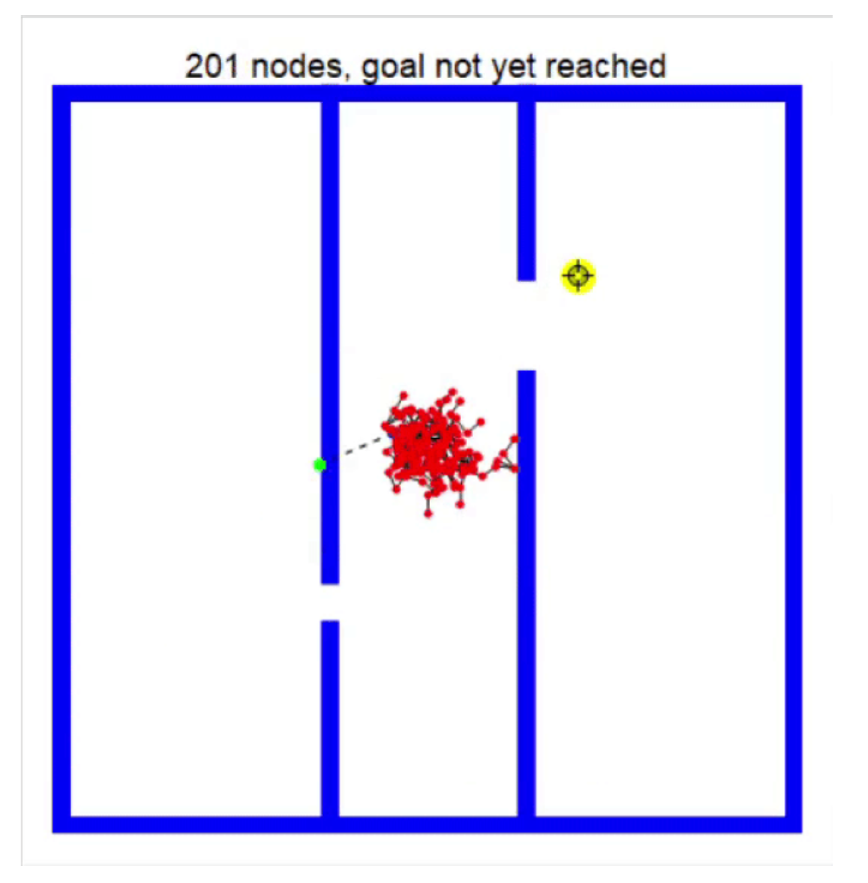
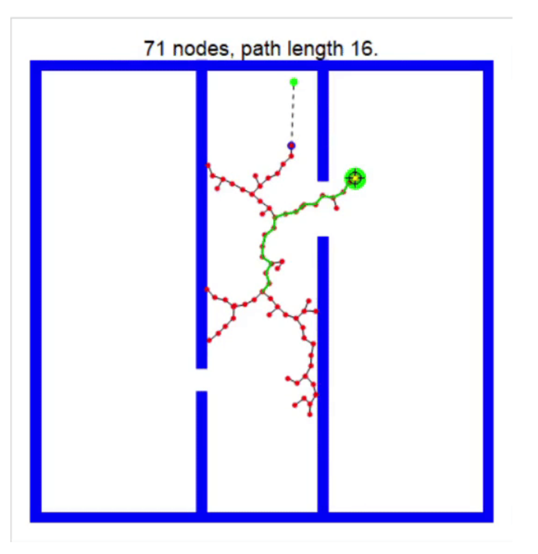
RRT expands heavily in unexplored portions of the configuration space of the robot when compared to naive random trees, who tend to expand heavily in places that are already explored (see Figure 2 and Figure 3). Thus, we can say that RRT is biased to unexplored regions. The vertices of RRT follow a uniform distribution. The algorithm is relatively simple and RRTs always stay connected even though the number of edges is minimal.
Since RRT algorithms are able to cope with non-holonomic constraints, they can be applied to almost any wheeled system. Depending on the user’s needs, they can select a variant of RRTs [59].
RRT Connect or bi-directional RRTs combine two RRTs, one at the starting position and a second at the goal position, connecting them using a heuristic. This approach is suitable for problems not involving differential constraints. During each iteration, one tree is extended, and the new vertex is connected to the nearest vertex of the other tree. Then, each tree’s role is reversed with both the trees exploring the free configuration space. This algorithm is suitable to plan motions for a robotic arm with high degrees of freedom [60].
In Sensor-based Random Trees (SRTs), a road map of the explored area is created with an associated Safe Region (SR) [61,62]. The Local Safe Area(LSR) is detected by the sensors. Each node of the SRT consists of a free configuration with associated Local Safe Region. The safe region consists of all local safe regions. It is an estimate of the free space surrounding the robot at a given configuration. The shape of the LSR depends on the sensor characteristics (e.g., the angular resolution) of the robot. The LSR shape can be a ball or a star.
The tree is expanded towards randomly-selected directions such that the new configuration and the path reaching towards the test robot are contained in the local safe region of the node. During each iteration, sensor data is collected and analyzed to generate a plausible region estimating the free space surrounding the robot at the current configuration. Then, a new node containing the current configuration and LSR is added to the tree. Depending on the robot’s sensors, different perception techniques can be used. The star-shaped LSR exploration strategy is more accurate as proven experimentally [61].
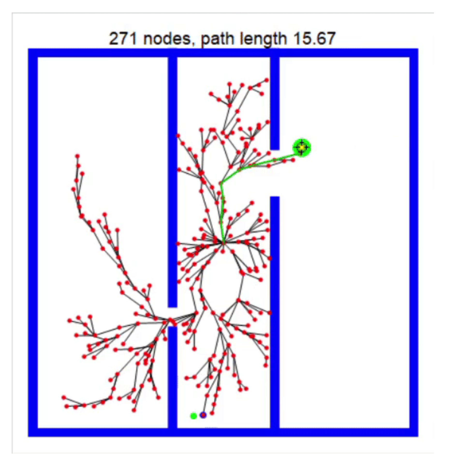
RRT* extends RRT to find the optimal path from a start to a goal node using triangle equality (see Figure 4). As the number of nodes increases, lower-cost (more optimal) paths are discovered. RRT-connect is particularly useful for robotic arms, like Programmable Universal Machine for Assembly (PUMA) robots [60]. The connect heuristic works most effectively when one can expect relatively open spaces for a majority of planning queries. The connect heuristic was originally developed with this kind of problem in mind [63]. Please see classification in Table 5 for RRT and its variants.
2.5. Genetic Algorithm
Discrete path planning algorithms, such as grid based algorithms and potential fields, require substantial CPU performance and/or require significant memory. In this section, we introduce genetic algorithms (GA), which help to overcome such limitations. For example, genetic algorithms can be applied with the advantage that such algorithms cover a large search space and use a minimal memory and CPU resources. They are also able to adapt to changing environments.
One disadvantage is that the solution found for the optimization problem may not always be a global minimum (e.g., the overall shortest path). One of the interesting applications of genetic algorithms is in small size humanoid robots that can play football [64]. We note that the robot needs to know the goal post in-order to kick the ball to the goal with the opposite team being obstacles, as the robot needs to avoid collisions and head towards the goal post to kick the ball into the goal. Thus, dynamic path planning is required in this case for the robot.
Since the algorithm is also applicable to dynamic environments, the optimal solution that finds a collision-free path between two points needs to be constantly updated according to change in surroundings. In this case, evolutionary methods converge upon an optimal solution. All possible solutions are represented as individuals of a population, with each gene representing a parameter. Individuals are formed by a complete set of genes.
A new generation is formed by selecting the best individuals from the parent generation and applying genetic operators, like crossover and mutation, to explore additional solutions. Each offspring from the new generation is tested with a fitness function devised for that problem. From all offspring, the best individuals are chosen as the parents of the next generation.
A fitness function is used to guide the simulation towards optimal design solutions. The fitness function must consider not only the shortest path but also the smoothness and clearance for dynamic path planning [65].
where and represent the weights on the total cost and , and are defined as follows:
where is the distance between two adjacent nodes
where is the angle between the extension of the two line segments connecting the ith knot point. is the desired steering angle, and a is a coefficient
where is the smallest distance from the ith segment to all the obstacles, and is the desired clearance distance.
Genetic operators are used to evolve plausible paths for selected parents. The selection operator chooses the fittest individuals and lets them pass their genes to the next generation. The crossover operator selects crossover point chosen at random from the genes for each pair of parents to be mated. The mutation operator performs the flipping of some bits in the bit string to maintain diversity. The GA produces the optimal path and takes advantage of the GA’s optimization ability [66]. Al-Taharwa et al. [67] described how to employ the GA approach in solving the path planning problem in a non-dynamic environment.
Their results showed that the hired method was efficient in handling the path planning problem in different static fields. The important characteristic that made GA suitable for solving these kinds of problem is that GA is an inherently parallel search method and has the capability to search for the optimal path in a given environment [66,68]. These are useful for path planning in complex environments containing U-shaped obstacles [69].
2.6. Ant Colony Algorithm
Computer Scientists and biologists have been inspired from nature for the design of path planning optimization algorithms. The ant colony optimization (ACO) algorithm, which is based on a heuristic approach inspired by the collective behavior of trail-laying ants to find the shortest and collision-free path, is one such derivative algorithm. This algorithm was first proposed by Marco Dorigo in his doctoral thesis “Ant system: by colony of cooperating agents” in 1992 [70] to simulate the ant foraging for food in Ant System (AS) theory.
According to the different characteristics of the problem, a variety of algorithms have been derived, which are probabilistic heuristic algorithms to find the shortest path. When ants forage for foods, they release a substance along the road, called pheromones, which are chemical substances. The following ants will then choose a suitable route according to the pheromone concentration left by the previous ants, and the probability of any ant to select the path is the same. When the concentration of existing pheromone is higher, the probability of ants to choose the path becomes higher as well.
However, the pheromone concentration becomes lower by evaporation. When the number of searches for paths increases, the shorter path will have a higher pheromone concentration because more ants have visited this path, while the other paths’ concentration will be lowered because less ants visit and there is a natural evaporation of the pheromones, which means that ants can search according to the pheromone information to move toward a path with shorter distances [71].
However, the ACO algorithm has a simple modeling process attributed to collective outcomes corresponding to many actions. The striking features of ACO algorithm are positive feedback helping in discovering a goal rapidly, distributed computation avoiding premature convergence, and greedy heuristics aiding in finding a goal in the early stages. The algorithm [70] is based on pheromone deposits, which determine the probability of an artificial ant to go from one node to another node in the path. The transition probability from node i to j is given by:
where is the pheromone level indicating the number of ants choosing the same edge as previously, is a heuristic indicating the closeness of the goal position, and and are weights determining the importance of the pheromones and heuristics.
Based on the application, the values of , , and are chosen to determine which neighboring nodes will be selected in the path to the goal. The more pheromone is present on a path, higher the probability for an ant to take that path. The ACO algorithm is used for robot dynamic path planning and exploited to find the pre-optimized path for the vehicle routing problem [72]. The traditional ant colony algorithm has a slow convergence speed due to the limitations of heuristic searches. In the application of vehicle path planning, it is easy to fall into a local optimal solution at the initial stage of optimization, resulting in stagnation.
The Enhanced Ant Colony Algorithm (EACA) [73] overcomes the shortcomings of the traditional ant colony algorithm, as ants move randomly in the process of searching for food and returning to the nest using state transition probability function (7). is the inspiration function of the node i from the node l. The purpose of modifying the inspiration function is to enhance the ant’s perceptions of the target node at the current node, which will guide ant to move to, thus, reduce the search time and avoid falling into a local optimum [74]. This algorithm can speed up the convergence and effectively generate reasonable solutions even in complex scenarios, which inspired people to use this in collision avoidance system with some more improvements in the ACO algorithm [75,76,77].
The Improved Ant Colony Optimization algorithm [78] executes a pheromone update method after each cycle of target search process, and the optimal path is planned using an improved cost function. The algorithm enhances the calculation ability of ACO and converges to optimal path much faster. It is used to solve large-scale fleet assignment problem and path planning for multiple automated guided vehicles (AGV) in a dynamic environment [78]. It is used for the optimal path planning of unmanned aerial vehicles (UAVs) [79] as it has better effectiveness in dynamic environments and more efficient use of computing power.
The Adaptive Ant Colony (AAC) algorithm [80] improves the ACO algorithm by adaptively updating the value of the evaporation rate, using Equation (8) and updating pheromone on each path, which is then fed to the transition probability Equation (7) to find the path direction.
where is a random number uniformly distributed in .
The AAC algorithm finds the global optimal path, better stability, convergence, and operational speed overcoming the defects of prematurity and stagnation in the ACO algorithm. To solve the vehicle routing problem, AAC has been used in conjunction with the Adaptive memory programming algorithm (AMP), where the algorithm is run in two iterations. The first iteration AMP is run so that it can cover the drawback of AAC falling into local minimum and on the result of AMP, i.e., a second iteration of AAC is run. By doing this, we have seen that the path length is minimized for vehicle path planning used in logistics [81].
The Bidirectional Ant Colony algorithm generates a global optimal path from two sets of paths generated by positive ants N and negative ants M from the original to the terminal and the terminal to the original node, respectively. The positive ant selects the nodes that have stronger pheromones whereas negative ants prefer weaker pheromone consistency using the improved transition probability formula [82].
As one group of ants is always towards the better nodes and another is always towards the poorer nodes, thus the poorer nodes will have the chance to be chosen. Secondly, in order to speed up the convergence of the latter part of the algorithm, the descending strategy is taken to reduce the scale of reverse ants and increase the scale of positive ants. Thereby, the positive ants search paths mainly, and the positive feedback is enhanced. Finally, each path can be optimized locally. The algorithm overcomes the problem of premature convergence and low convergence speed posed by the ACO algorithm.
Bio-inspired optimization methods resulted in the slime mold-based optimization algorithm (SLIMO). The SLIMO algorithm [83] mimics a true slime mold that connects food sources and distributes nutrients through a self-assembled resource distribution network of tubes with varying diameters evolving with changing environmental conditions. The advantage of SLIMO path planning is that only a partial re-growth followed by short tube dynamics needs to be conducted to find the optimal path automatically in response to a dynamic environment. The application ranges from evacuation planning in uncertain or hazardous environments to path planning for real-world infrastructure networks—e.g., the Tokyo rail system [84].
ACO algorithm and its variants are types of parallel optimization algorithms, and thus they have good convergence and global optimization performance. The adaptive ant colony algorithm has a good global optimization ability, and it exhibits better optimization performance compared to other variants of the ACO algorithm. Please see classification in Table 6 for ACO and its variants.
2.7. Firefly Algorithm
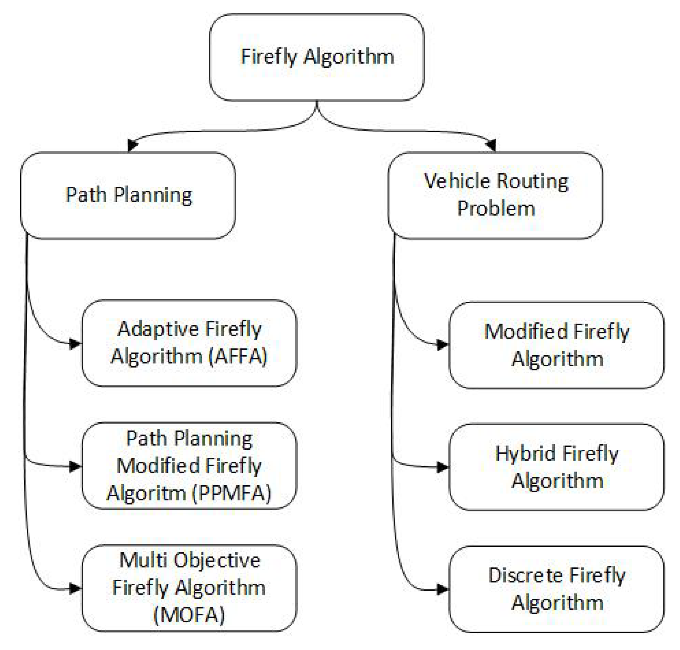
The Firefly algorithm is a meta-heuristic algorithm based on Firefly mating behavior. It is a promising swarm-intelligence-based algorithm inspired by the collective behavior of insects or animals who cooperate in order to solve complex problems. Colonies of insects act as decentralized, self-organized systems that prevent a single insect from acting. The algorithm is used for solving continuous and discrete optimization problems [85]. In order to tackle optimization problems efficiently, many variants of the Firefly algorithm have been developed, see Figure 5.
The Firefly algorithm works on huge data sets and can be applied on path planning. Path planning can widely be divided into two branches: Global Path Planning [86] and Local Path Planning. Global planning is done on a larger set, and calculation of the shortest path is done from the start node to the goal node. The Local Planner begins when an obstacle is found to move around, and this is done on previous nodes and near nodes, which are available in the global set.
The Modified Firefly Algorithm (MFA) is appropriate for global path planning and has yielded better results [88] as Modified Firefly uses a Gaussian random walk to replace the fixed-size step of the Standard Firefly Algorithm (SFA). Multiple checking methods enhance the success of the Firefly movement during the iteration process. The Modified Firefly algorithm overcomes one of the weaknesses of the conventional Firefly algorithm, which is slow convergence.
The number of iterations that are required is based on the distance between two fireflies and the intensity of the next brightest Firefly, enabling faster convergence during the final stages of the search. The complexity of three-dimensional (3D) path planning for Autonomous Underwater Vehicles (AUVs) requires optimization algorithms. The required optimization algorithm must have a fast convergence speed. The modified Firefly algorithm overcomes the convergence slowness of the basic Firefly algorithm. This is helpful in 3D underwater planning as we can achieve faster optimization [87].
The Adaptive Firefly Algorithm (AFA) was proposed [89] by utilizing the composite benefit of Firefly Algorithm (FA) for global exploration and Temporal Difference Q-Learning (TDQL) for local tuning of the absorption coefficient. A relative comparison AFA technique with classical FA and Particle Swarm Optimization (PSO) demonstrated that the AFA algorithm outperformed all its competitors with respect to accuracy and the run-time required for convergence [89].
The Developed Firefly Algorithm (DFA) provides a shorter path length and path smoothness in multi-objective path planning [90]. In SFA, the attraction of the fireflies is depended by the Euclidean distance. However in DFA, the Pareto-based method (here, the objective function is no longer a scalar value, but rather a vector) is used to estimate the brightness of the fireflies. By using this approach it helps to balance the optimized solution, yielding a smooth passable path as the result.
The Firefly algorithm is often used where large data sets exist and is suitable for dynamic environments. As discussed above, the Firefly algorithm is very popular in AUVs [89] where a 3D optimal path is found from the start point to the destination with the shortest path length and with collision free navigation with any obstacles in the working space. Please see classification in Table 7 for Firefly and its variants.
3. Conclusions
Recent years have seen the rapid growth of artificial intelligence in driverless vehicles and other automated mobile systems. As a result, the amount of research into path planning has increased dramatically. In the last decade, many new methods of path planning have been developed; however, it is difficult to find a comprehensive survey on the most popular path planning algorithms suitable for the novice practitioner.
In this paper, we presented several widely used path planning algorithms and their variants, categorized based primarily upon whether the environment in which the robot operates is static or dynamic. In each section, we covered the methodology of all the algorithms as well as their advantages and disadvantages, creating a comparative table in each section for where each algorithm was suited best based on a static or dynamic environment. The advances in computing and perception hardware have enabled us to use complex algorithms for path planning.
As both D* Lite and Enhanced D* Lite are based on A* it could be concluded that the added complexity tends to cost computational time [91]. Field D* is one such algorithm that stands out as one of the best algorithms suited for a dynamic environment as this is shown to decrease the computational time significantly. This helps in the presence of dynamic obstacles where the reaction time is very important, particularly with faster moving dynamic obstacles.
We conclude that, for a given map the algorithm A* is a strong-performing option for static environments because of the low memory usage, computational speed, less implementation complexity, and efficiency making it suitable also for use in embedded system deployment. One of the main limitations of bio-inspired algorithms is that they do not have excellent results in real-time path planning as they have a possibility of becoming stuck in local minima.
It is our hope that the reader, having witnessed a brief survey of the path planning landscape for AVs and other mobile robotic systems, will gain an awareness of the vocabulary needed and design considerations to take into account in designing, comparing, and implementing a path planning system with particular goals and constraints.
Though not exhaustive, this coverage provides a simplified summary for these techniques and their use cases and trade-offs to help readers become up-to-speed quickly such that a system might be implemented rapidly and safely and be optimized over time. The field of path planning continues to grow, and we encourage readers to seek out the latest and greatest algorithms suitable for their respective domains after reading this primer text.
Author Contributions
Conceptualization, K.K., N.S. and C.D.; methodology, K.K., N.S., C.D. and J.E.S.; investigation, K.K., N.S. and C.D.; writing—original draft preparation, K.K., N.S. and C.D.; writing—review and editing, K.K., N.S., C.D. and J.E.S.; visualization, K.K.; supervision, J.E.S.; project administration, J.E.S. and K.K. All authors have read and agreed to the published version of the manuscript.
Funding
There was no external funding provided for this research.
Institutional Review Board Statement
Not applicable.
Informed Consent Statement
Not applicable.
Data Availability Statement
Not applicable.
Conflicts of Interest
The authors declare no known conflicts of interest.
References
- Zheng, C.; Green, R. Vision-based autonomous navigation in indoor environments. In Proceedings of the 2010 25th International Conference of Image and Vision Computing New Zealand, Queenstown, New Zealand, 8–9 November 2010; pp. 1–7. [Google Scholar] [CrossRef]
- Sariff, N.; Buniyamin, N. An Overview of Autonomous Mobile Robot Path Planning Algorithms. In Proceedings of the 2006 4th Student Conference on Research and Development, Shah Alam, Malaysia, 27–28 June 2006; pp. 183–188. [Google Scholar] [CrossRef]
- Sariff, N.; Buniyamin, N. Ant colony system for robot path planning in global static environment. In Proceedings of the 9th WSEAS International Conference on System Science and Simulation in Engineering (ICOSSSE’10), Takizawa, Japan, 4–6 October 2010; pp. 192–197. [Google Scholar]
- Mac, T.; Copot, C.; Tran, D.; Keyser, R. Heuristic approaches in robot path planning: A survey. Robot. Auton. Syst. 2016, 86. [Google Scholar] [CrossRef]
- Chen, B.; Quan, G. NP-Hard Problems of Learning from Examples. In Proceedings of the 2008 Fifth International Conference on Fuzzy Systems and Knowledge Discovery, Jinan, China, 8–20 October 2008; Volume 2, pp. 182–186. [Google Scholar] [CrossRef]
- Klančar, G.; Zdešar, A.; Blazic, S. Wheeled Mobile Robotics; Butterworth-Heinemann: Oxford, UK, 2017. [Google Scholar]
- Janet, J.A.; Luo, R.C.; Kay, M.G. The essential visibility graph: An approach to global motion planning for autonomous mobile robots. In Proceedings of the 1995 IEEE International Conference on Robotics and Automation, Nagoya, Japan, 21–27 May 1995; Volume 2, pp. 1958–1963. [Google Scholar] [CrossRef]
- Dijkstra, E. A note on two problems in connexion with graphs. Numer. Math. 1959, 1, 269–271. [Google Scholar] [CrossRef] [Green Version]
- Zhang, Y.; Tang, G.; Chen, L. Improved A* Algorithm For Time-dependent Vehicle Routing Problem. In Proceedings of the 2012 International Conference on Computer Application and System Modeling, ICCASM 2012, Taiyuan, China, 27–29 July 2012. [Google Scholar] [CrossRef] [Green Version]
- Hart, P.E.; Nilsson, N.J.; Raphael, B. A Formal Basis for the Heuristic Determination of Minimum Cost Paths. IEEE Trans. Syst. Sci. Cybern. 1968, 4, 100–107. [Google Scholar] [CrossRef]
- Dudi, T.; Singhal, R.; Kumar, R. Shortest Path Evaluation with Enhanced Linear Graph and Dijkstra Algorithm. In Proceedings of the 2020 59th Annual Conference of the Society of Instrument and Control Engineers of Japan (SICE); 2020; pp. 451–456. Available online: https://sice2020.sice.jp/ (accessed on 9 October 2020).
- Stentz, A. Optimal and efficient path planning for partially known environments. In Intelligent Unmanned Ground Vehicles; Springer: Berlin/Heidelberg, Germany, 1997; pp. 203–220. [Google Scholar]
- LaValle, S.M. Rapidly-Exploring Random Trees: A New Tool for Path Planning. 1998. Available online: http://lavalle.pl/papers/Lav98c.pdf (accessed on 9 October 2020).
- Ammar, A.; Bennaceur, H.; Chaari, I.; Koubaa, A.; Alajlan, M. Relaxed Dijkstra and A* with linear complexity for robot path planning problems in large-scale grid environments. Soft Comput. 2015, 20, 1–23. [Google Scholar] [CrossRef]
- Majeed, A.; Hwang, S.O. Path Planning Method for UAVs Based on Constrained Polygonal Space and an Extremely Sparse Waypoint Graph. Appl. Sci. 2021, 11, 5340. [Google Scholar] [CrossRef]
- Gbadamosi, O.A.; Aremu, D.R. Design of a Modified Dijkstra’s Algorithm for finding alternate routes for shortest-path problems with huge costs. In Proceedings of the 2020 International Conference in Mathematics, Computer Engineering and Computer Science (ICMCECS), Lagos, Nigeria, 18–21 March 2020; pp. 1–6. [Google Scholar] [CrossRef]
- Qing, G.; Zheng, Z.; Yue, X. Path-planning of automated guided vehicle based on improved Dijkstra algorithm. In Proceedings of the 2017 29th Chinese control and decision conference (CCDC), Chongqing, China, 28–30 May 2017; pp. 7138–7143. [Google Scholar] [CrossRef]
- Syed Abdullah, F.; Iyal, S.; Makhtar, M.; Jamal, A.A. Robotic Indoor Path Planning Using Dijkstra’s Algorithm with Multi-Layer Dictionaries. In Proceedings of the 2015 2nd International Conference on Information Science and Security (ICISS), Seoul, Korea, 14–16 December 2015. [Google Scholar] [CrossRef]
- Kang, H.; Lee, B.h.; Kim, K. Path Planning Algorithm Using the Particle Swarm Optimization and the Improved Dijkstra Algorithm. In Proceedings of the 2008 IEEE Pacific-Asia Workshop on Computational Intelligence and Industrial Application, Wuhan, China, 19–20 December 2009; Volume 18, pp. 1002–1004. [Google Scholar] [CrossRef]
- Fuhao, Z.; Jiping, L. An Algorithm of Shortest Path Based on Dijkstra for Huge Data. In Proceedings of the 2009 Sixth International Conference on Fuzzy Systems and Knowledge Discovery, Tianjin, China, 14–16 August 2009; Volume 4, pp. 244–247. [Google Scholar] [CrossRef]
- Fu, M.; Li, J.; Deng, Z. A practical route planning algorithm for vehicle navigation system. In Proceedings of the Fifth World Congress on Intelligent Control and Automation (IEEE Cat. No.04EX788), Hangzhou, China, 15–19 June 2004; Volume 6, pp. 5326–5329. [Google Scholar] [CrossRef]
- Silva, M.C.; Garcia, A.C.B.; Conci, A. A Multi-agent System for Dynamic Path Planning. In Proceedings of the 2010 Second Brazilian Workshop on Social Simulation, Sao Paulo, Brazil, 24–25 October 2010; pp. 47–51. [Google Scholar] [CrossRef]
- Ferguson, D.; Likhachev, M.; Stentz, A. A Guide to Heuristic-based Path Planning. In Proceedings of the International Workshop on Planning under Uncertainty for Autonomous Systems, International Conference on Automated Planning and Scheduling (ICAPS), Monterey, CA, USA, 5–10 June 2005; pp. 9–18. [Google Scholar]
- Gass, S.I.; Harris, C.M. Near-optimal solution. In Encyclopedia of Operations Research and Management Science; Gass, S.I., Harris, C.M., Eds.; Springer: New York, NY, USA, 2001; p. 555. [Google Scholar] [CrossRef]
- Hernández, C.; Baier, J.; Achá, R. Making A* run faster than D*-lite for path-planning in partially known terrain. In Proceedings of the International Conference on Automated Planning and Scheduling, ICAPS, Portsmouth, NH, USA, 21–26 June 2014; Volume 2014, pp. 504–508. [Google Scholar]
- Cui, X.; Shi, H. A*-based Pathfinding in Modern Computer Games. Int. J. Comput. Sci. Netw. Secur. 2010, 11, 125–130. [Google Scholar]
- Gunawan, S.A.; Pratama, G.N.P.; Cahyadi, A.I.; Winduratna, B.; Yuwono, Y.C.H.; Wahyunggoro, O. Smoothed A-star Algorithm for Nonholonomic Mobile Robot Path Planning. In Proceedings of the 2019 International Conference on Information and Communications Technology (ICOIACT); 2019; pp. 654–658. Available online: https://icoiact.org/ (accessed on 9 October 2020). [CrossRef]
- Zhou, Y.; Cheng, X.; Lou, X.; Fang, Z.; Ren, J. Intelligent Travel Planning System based on A-star Algorithm. In Proceedings of the 2020 IEEE 4th Information Technology, Networking, Electronic and Automation Control Conference (ITNEC), Chongqing, China, 12–14 June 2020; Volume 1, pp. 426–430. [Google Scholar] [CrossRef]
- Belhaous, S.; Baroud, S.; Chokri, S.; Hidila, Z.; Naji, A.; Mestari, M. Parallel implementation of A* search algorithm for road network. In Proceedings of the 2019 Third International Conference on Intelligent Computing in Data Sciences (ICDS), Marrakech, Morocco, 28–30 October 2019; pp. 1–7. [Google Scholar] [CrossRef]
- Dong, G.; Yang, F.; Tsui, K.L.; Zou, C. Active Balancing of Lithium-Ion Batteries Using Graph Theory and A-Star Search Algorithm. IEEE Trans. Ind. Inform. 2021, 17, 2587–2599. [Google Scholar] [CrossRef]
- Liu, H.; Shan, T.; Wang, W. Automatic Routing Study of Spacecraft Cable based on A-star Algorithm. In Proceedings of the 2020 IEEE 5th Information Technology and Mechatronics Engineering Conference (ITOEC), Chongqing, China, 12–14 June 2020; pp. 716–719. [Google Scholar] [CrossRef]
- Kider, J.T.; Henderson, M.; Likhachev, M.; Safonova, A. High-dimensional planning on the GPU. In Proceedings of the 2010 IEEE International Conference on Robotics and Automation, Anchorage, AK, USA, 3–7 May 2010; pp. 2515–2522. [Google Scholar] [CrossRef] [Green Version]
- Cheng, L.; Liu, C.; Yan, B. Improved hierarchical A-star algorithm for optimal parking path planning of the large parking lot. In Proceedings of the 2014 IEEE International Conference on Information and Automation (ICIA), Hailar, Hulun Buir, China, 28–30 July 2014; pp. 695–698. [Google Scholar] [CrossRef]
- Yao, J.; Lin, C.; Xie, X.; Wang, A.; Hung, C.C. Path Planning for Virtual Human Motion Using Improved A* Star Algorithm. In Proceedings of the 2010 Seventh International Conference on Information Technology: New Generations, Las Vegas, NV, USA, 12–14 April 2010; pp. 1154–1158. [Google Scholar] [CrossRef]
- Chen, T.; Zhang, G.; Hu, X.; Xiao, J. Unmanned aerial vehicle route planning method based on a star algorithm. In Proceedings of the 2018 13th IEEE Conference on Industrial Electronics and Applications (ICIEA), Wuhan, China, 31 May–2 June 2018; pp. 1510–1514. [Google Scholar] [CrossRef]
- Goto, T.; Kosaka, T.; Noborio, H. On the heuristics of A* or A algorithm in ITS and robot path-planning. In Proceedings of the 2003 IEEE/RSJ International Conference on Intelligent Robots and Systems (IROS 2003) (Cat. No.03CH37453), Las Vegas, NV, USA, 27–31 October 2003; Volume 2, pp. 1159–1166. [Google Scholar]
- Sedighi, S.; Nguyen, D.V.; Kuhnert, K.D. Guided Hybrid A-star Path Planning Algorithm for Valet Parking Applications. In Proceedings of the 2019 5th International Conference on Control, Automation and Robotics (ICCAR), Beijing, China, 19–22 April 2019; pp. 570–575. [Google Scholar] [CrossRef]
- LaValle, S.M. Planning Algorithms; Cambridge University Press: Cambridge, UK, 2006. [Google Scholar]
- De Berg, M.; van Kreveld, M.; Overmars, M.; Schwarzkopf, O. Computational Geometry: Algorithms and Applications, 2nd ed.; Springer: Berlin/Heidelberg, Germany, 2000; p. 367. [Google Scholar]
- Yijing, W.; Zhengxuan, L.; Zhiqiang, Z.; Zheng, L. Local Path Planning of Autonomous Vehicles Based on A* Algorithm with Equal-Step Sampling. In Proceedings of the 2018 37th Chinese Control Conference (CCC), Wuhan, China, 25–27 July 2018; pp. 7828–7833. [Google Scholar] [CrossRef]
- Koenig, S.; Likhachev, M.; Furcy, D. Lifelong Planning A*. Artif. Intell. 2004, 155, 93–146. [Google Scholar] [CrossRef] [Green Version]
- Xie, K.; Qiang, J.; Yang, H. Research and Optimization of D-Start Lite Algorithm in Track Planning. IEEE Access 2020, 8, 161920–161928. [Google Scholar] [CrossRef]
- Baker, Z.K.; Gokhale, M. On the Acceleration of Shortest Path Calculations in Transportation Networks. In Proceedings of the 15th Annual IEEE Symposium on Field-Programmable Custom Computing Machines (FCCM 2007), Piscataway, NJ, USA, 23–25 April 2007; pp. 23–34. [Google Scholar] [CrossRef]
- Seo, W.; Ok, S.; Ahn, J.; Kang, S.; Moon, B. An Efficient Hardware Architecture of the A-star Algorithm for the Shortest Path Search Engine. In Proceedings of the 2009 Fifth International Joint Conference on INC, IMS and IDC, Seoul, Korea, 25–27 August 2009; pp. 1499–1502. [Google Scholar] [CrossRef]
- Stentz, A. Optimal and Efficient Path Planning for Unknown and Dynamic Environments; The Robotics Instilute Carnegie Mellon University: Pittsburge, PA, USA, 2003; Volume 10. [Google Scholar]
- Nilsson, N.J. Principles of Artificial Intelligence; Morgan Kaufmann Publishers Inc.: San Francisco, CA, USA, 1980. [Google Scholar]
- Stentz, A. The D* Algorithm for Real-Time Planning of Optimal Traverses. 2011. Available online: https://www.ri.cmu.edu/pub_files/pub3/stentz_anthony__tony__1994_2/stentz_anthony__tony__1994_2.pdf (accessed on 9 October 2020).
- Koenig, S.; Likhachev, M. D*Lite. In Eighteenth National Conference on Artificial Intelligence; American Association for Artificial Intelligence: Menlo Park, CA, USA, 2002; pp. 476–483. [Google Scholar]
- Wang, J.; Garratt, M.A.; Anavatti, S.G. Dynamic path planning algorithm for autonomous vehicles in cluttered environments. In Proceedings of the 2016 IEEE International Conference on Mechatronics and Automation, Harbin, China, 7–10 August 2016; pp. 1006–1011. [Google Scholar]
- Yun, S.C. Enhanced D * Lite Algorithm for Autonomous Mobile Robot Velappa Ganapathy. 2011. Available online: https://www.researchgate.net/publication/251979681_Enhanced_D_Lite_Algorithm_for_mobile_robot_navigation (accessed on 9 October 2020).
- Larson, R.E.; Casti, J.L. Principles of Dynamic Programming; M. Dekker: New York, NY, USA, 1978; p. 2. [Google Scholar]
- Larson, R. A survey of dynamic programming computational procedures. IEEE Trans. Autom. Control 1967, 12, 767–774. [Google Scholar] [CrossRef]
- Ferguson, D.; Stentz, A. Field D*: An Interpolation-Based Path Planner and Replanner. In Robotics Research; Springer: Berlin/Heidelberg, Germany, 2005; Volume 28, pp. 239–253. [Google Scholar] [CrossRef] [Green Version]
- Zlot, R.; Stentz, A.; Dias, M.B.; Thayer, S. Multi-robot exploration controlled by a market economy. In Proceedings of the 2002 IEEE International Conference on Robotics and Automation (Cat. No.02CH37292), Washington, DC, USA, 11–15 May 2002; Volume 3, pp. 3016–3023. [Google Scholar] [CrossRef]
- Thayer, S.; Dias, M.; Nabbe, B.; Digney, B.; Hebert, M.; Stentz, A. Distributed Robotic Mapping of Extreme Environments. Proceedings of SPIE—The International Society for Optical Engineering; 2001; Volume 4195. Available online: https://www.spiedigitallibrary.org/conference-proceedings-of-spie/4195/0000/Distributed-robotic-mapping-of-extreme-environments/10.1117/12.417292.short?SSO=1 (accessed on 9 October 2020). [CrossRef]
- Singh, S.; Simmons, R.; Smith, T.; Stentz, A.; Verma, V.; Yahja, A.; Schwehr, K. Recent progress in local and global traversability for planetary rovers. In Proceedings of the 2000 ICRA. Millennium Conference. IEEE International Conference on Robotics and Automation. Symposia Proceedings (Cat. No.00CH37065), San Francisco, CA, USA, 24–28 April 2000; Volume 2, pp. 1194–1200. [Google Scholar] [CrossRef] [Green Version]
- LaValle, S.M.; Kuffner, J.J., Jr. Randomized kinodynamic planning. Int. J. Robot. Res. 2001, 20, 378–400. [Google Scholar] [CrossRef]
- Huang, L. Rapidly Exploring Random Tree (RRT) and RRT*. 2018. Available online: http://wolfram.com/knowledgebase/source-information (accessed on 20 March 2019).
- Souissi, O.; Benatitallah, R.; Duvivier, D.; Artiba, A.; Belanger, N.; Feyzeau, P. Path planning: A 2013 survey. In Proceedings of the 2013 International Conference on Industrial Engineering and Systems Management (IESM), Rabat, Morocco, 28–30 October 2013; pp. 1–8. [Google Scholar]
- Kuffner, J.J.; LaValle, S.M. RRT-connect: An efficient approach to single-query path planning. In Proceedings of the 2000 ICRA. Millennium Conference. IEEE International Conference on Robotics and Automation. Symposia Proceedings (Cat. No. 00CH37065), San Francisco, CA, USA, 24–28 April 2000; Volume 2, pp. 995–1001. [Google Scholar]
- Oriolo, G.; Vendittelli, M.; Freda, L.; Troso, G. The SRT method: Randomized strategies for exploration. In Proceedings of the IEEE International Conference on Robotics and Automation, 2004. Proceedings. ICRA ’04, New Orleans, LA, USA, 26 April–1 May 2004; Volume 5, pp. 4688–4694. [Google Scholar] [CrossRef] [Green Version]
- Yiping, Z.; Jian, G.; Ruilei, Z.; Qingwei, C. A SRT-based path planning algorithm in unknown complex environment. In Proceedings of the 26th Chinese Control and Decision Conference (2014 CCDC), Changsha, China, 31 May–2 June 2014; pp. 3857–3862. [Google Scholar] [CrossRef]
- Kuner, J.; Latombe, J.c.; Guibas, L.; Bregler, C. Autonomous Agents For Real-Time Animation. Ph.D. Thesis, Stanford University, Stanford, CA, USA, 2000. [Google Scholar]
- Burchardt, H.; Salomon, R. Implementation of Path Planning using Genetic Algorithms on Mobile Robots. In Proceedings of the 2006 IEEE International Conference on Evolutionary Computation, Vancouver, BC, Canada, 16–21 July 2006; pp. 1831–1836. [Google Scholar] [CrossRef]
- Elshamli, A.; Abdullah, H.A.; Areibi, S. Genetic algorithm for dynamic path planning. In Proceedings of the Canadian Conference on Electrical and Computer Engineering 2004 (IEEE Cat. No.04CH37513), Niagara Falls, ON, Canada, 2–5 May 2004; Volume 2, pp. 677–680. [Google Scholar] [CrossRef]
- Samadi, M.; Othman, M.F. Global Path Planning for Autonomous Mobile Robot Using Genetic Algorithm. In Proceedings of the 2013 International Conference on Signal-Image Technology Internet-Based Systems, Kyoto, Japan, 2–5 December 2013; pp. 726–730. [Google Scholar] [CrossRef]
- L-Taharwa, I.A.; Sheta, A.; Al-Weshah, M. A Mobile Robot Path Planning Using Genetic Algorithm in Static Environment. J. Comput. Sci. 2008, 4, 341–344. [Google Scholar] [CrossRef] [Green Version]
- Thomaz, C.; Pacheco, M.; Vellasco, M. Mobile robot path planning using genetic algorithms. In International Work-Conference on Artificial Neural Networks; Springer: Berlin/Heidelberg, Germany, 2006; Volume 1606, pp. 671–679. [Google Scholar] [CrossRef]
- Yanrong, H.; Yang, S.X. A knowledge based genetic algorithm for path planning of a mobile robot. In Proceedings of the IEEE International Conference on Robotics and Automation, 2004. Proceedings. ICRA ’04. 2004, New Orleans, LA, USA, 26 April–1 May 2004; Volume 5, pp. 4350–4355. [Google Scholar] [CrossRef]
- Dorigo, M.; Maniezzo, V.; Colorni, A. Ant system: Optimization by a colony of cooperating agents. IEEE Trans. Syst. Man Cybern. Part B (Cybern.) 1996, 26, 29–41. [Google Scholar] [CrossRef] [PubMed] [Green Version]
- Yu, K.; Lee, M.; Chi, S. Dynamic path planning based on adaptable Ant colony optimization algorithm. In Proceedings of the 2017 Sixth International Conference on Future Generation Communication Technologies (FGCT), Dublin, Ireland, 21–23 August 2017; pp. 1–7. [Google Scholar] [CrossRef]
- Meng, L.; Lin, C.; Huang, H.; Cai, X. Vehicle routing plan based on ant colony and insert heuristic algorithm. In Proceedings of the 2016 35th Chinese Control Conference (CCC), Chengdu, China, 27–29 July 2016; pp. 2658–2662. [Google Scholar] [CrossRef]
- Zhou, Z.; Nie, Y.; Min, G. Enhanced Ant Colony Optimization Algorithm for Global Path Planning of Mobile Robots. In Proceedings of the 2013 International Conference on Computational and Information Sciences, Shiyan, China, 21–23 June 2013; pp. 698–701. [Google Scholar] [CrossRef]
- Wang, Y.; Lu, X.; Zuo, Z. Autonomous Vehicles Path Planning With Enhanced Ant Colony optimization. In Proceedings of the 2019 Chinese Control Conference (CCC), Guangzhou, China, 27–30 July 2019; pp. 6633–6638. [Google Scholar] [CrossRef]
- Wang, H.; Guo, F.; Yao, H.; He, S.; Xu, X. Collision Avoidance Planning Method of USV Based on Improved Ant Colony Optimization Algorithm. IEEE Access 2019, 7, 52964–52975. [Google Scholar] [CrossRef]
- Huadong, Z.; Chaofan, L.; Nan, J. A Path Planning Method of Robot Arm Obstacle Avoidance Based on Dynamic Recursive Ant Colony Algorithm. In Proceedings of the 2019 IEEE International Conference on Power, Intelligent Computing and Systems (ICPICS), Shenyang, China, 12–14 July 2019; pp. 549–552. [Google Scholar] [CrossRef]
- He, J.; Wang, H.; Liu, C.; Yu, D. UUV Path Planning for Collision Avoidance Based on Ant Colony Algorithm. In Proceedings of the 2020 39th Chinese Control Conference (CCC), Shenyang, China, 27–29 July 2020; pp. 5528–5533. [Google Scholar] [CrossRef]
- Juntao, L.; Tingting, D.; Yuanyuan, L.; Yan, H. Study on Robot Path Collision Avoidance Planning Based on the Improved Ant Colony Algorithm. In Proceedings of the 2016 8th International Conference on Intelligent Human-Machine Systems and Cybernetics (IHMSC), Hangzhou, China, 27–28 August 2016; Volume 2, pp. 540–544. [Google Scholar] [CrossRef]
- Qiannan, Z.; Ziyang, Z.; Chen, G.; Ruyi, D. Path planning of UAVs formation based on improved ant colony optimization algorithm. In Proceedings of the 2014 IEEE Chinese Guidance, Navigation and Control Conference, Yantai, China, 8–10 August 2014; pp. 1549–1552. [Google Scholar] [CrossRef]
- Chen, M. Toward Adaptive Ant Colony Algorithm. In Proceedings of the 2010 International Conference on Measuring Technology and Mechatronics Automation, Changsha, China, 13–14 March 2010; Volume 3, pp. 1035–1038. [Google Scholar] [CrossRef]
- Wang, R.; Zheng, D.; Zhang, H.; Mao, J.; Guo, N. A solution for simultaneous adaptive ant colony algorithm to memory demand vehicle routing problem with pickups. In Proceedings of the 2016 Chinese Control and Decision Conference (CCDC), Yinchuan, China, 28–30 May 2016; pp. 2172–2176. [Google Scholar] [CrossRef]
- Wu, Y.; Shi, L.; Li, Q.; Chen, Y. Novel path planning of robots based on bidirectional ant colony algorithm. In Proceedings of the 2010 Sixth International Conference on Natural Computation, Yantai, China, 10–12 August 2010; Volume 5, pp. 2403–2406. [Google Scholar] [CrossRef]
- Kropat, E.; Meyer-Nieberg, S. A Multi-layered Adaptive Network Approach for Shortest Path Planning During Critical Operations in Dynamically Changing and Uncertain Environments. In Proceedings of the 2016 49th Hawaii International Conference on System Sciences (HICSS), Koloa, HI, USA, 5–8 January 2016; pp. 1369–1378. [Google Scholar] [CrossRef]
- Tero, A.; Takagi, S.; Saigusa, T.; Ito, K.; Bebber, D.; Fricker, M.; Yumiki, K.; Kobayashi, R.; Nakagaki, T. Rules for Biologically Inspired Adaptive Network Design. Science 2010, 327, 439–442. [Google Scholar] [CrossRef] [PubMed] [Green Version]
- Fister, I., Jr.; Perc, M.; Kamal, S.; Fister, I. A review of chaos-based Firefly algorithms: Perspectives and research challenges. Appl. Math. Comput. 2015, 252. [Google Scholar] [CrossRef]
- Fister, I.; Fister, I., Jr.; Yang, X.S.; Brest, J. A comprehensive review of Firefly algorithms. Swarm Evol. Comput. 2013, 13, 34–46. [Google Scholar] [CrossRef] [Green Version]
- Chandrawati, T.; Sari, R. A Review of Firefly Algorithms for Path Planning, Vehicle Routing and Traveling Salesman Problems. In Proceedings of the 2018 2nd International Conference on Electrical Engineering and Informatics (ICon EEI), Batam, Indonesia, 16–17 October 2019. [Google Scholar] [CrossRef]
- Chen, X.; Zhou, M.; Huang, J.; Luo, Z. Global path planning using modified Firefly algorithm. In Proceedings of the 2017 International Symposium on Micro-NanoMechatronics and Human Science (MHS), Nagoya, Japan, 3–6 December 2017; pp. 1–7. [Google Scholar] [CrossRef]
- Ghosh Roy, A.; Rakshit, P.; Konar, A.; Bhattacharya, S.; Kim, E.; Nagar, A. Adaptive Firefly Algorithm for nonholonomic motion planning of car-like system. In Proceedings of the 2013 IEEE Congress on Evolutionary Computation, Cancun, Mexico, 20–23 June 2013; pp. 2162–2169. [Google Scholar] [CrossRef]
- Duan, P.; Li, J.; Sang, H.; Han, Y.; Sun, Q. A Developed Firefly Algorithm for Multi-Objective Path Planning Optimization Problem. In Proceedings of the 2018 IEEE 8th Annual International Conference on CYBER Technology in Automation, Control, and Intelligent Systems (CYBER), Tianjin, China, 19 July–23 July 2018; pp. 1393–1397. [Google Scholar] [CrossRef]
- Anavatti, S.G.; Biswas, S.; Colvin, J.T.; Pratama, M. A hybrid algorithm for efficient path planning of autonomous ground vehicles. In Proceedings of the 2016 14th International Conference on Control, Automation, Robotics and Vision (ICARCV), Phuket, Thailand, 13–15 November 2016; pp. 1–6. [Google Scholar] [CrossRef]
Short Biography of Authors
Karthik Karur received the bachelor’s degree from the Visvesvaraya Technological University Belguam, Karnataka, India, and the Master’s from Illinois Institute of Technology, Chicago, USA in 2007 and 2010, respectively. He is currently pursuing Ph.D. degree in Electrical and Computer Engineering from Michigan State University, East Lansing, MI, USA. He also works as an Embedded Software Engineer with Halla Mechatronics, Bay City, MI, USA, where he focuses on developing motor control algorithms and lead integrator for automotive software. His current research interests include machine learning, motor control, sensor fusion, and artificial intelligence.
Chinmay Dharmatti received the bachelor’s degree in Electronics and Telecommunications Engineering from the University of Pune, India, in 2017 and a Master’s degree in Electrical and Computer Engineering from Michigan State University in 2020. He is currently working at Halla Mechatronics as a Controls engineer with a focus on precision motor control. His areas of interest include optimization and control theory, robotics and artificial intelligence.
Nitin Sharma received the bachelor’s degree from the SRM University, Chennai, India in 2013 and currently pursuing a Master’s degree from the Michigan State University. He has worked with Johnson Controls as Systems Engineer on various key projects in HVAC. He is currently working as an administrative intern with Changan US Research and Development Center in Plymouth, MI. His areas of interest include control systems and robotics.
Joshua E. Siegel received the bachelor’s, master’s, and Ph.D. degrees from the Massachusetts Institute of Technology in 2011, 2013, and 2016, respectively. He is an Assistant Professor in the Computer Science and Engineering Department at Michigan State University where he leads the Deep Tech Lab. His research interests include connected vehicles, pervasive sensing, and secure and efficient architectures for the Internet of Things. He received the Lemelson-MIT National Collegiate Student “Drive It” Prize in 2015.
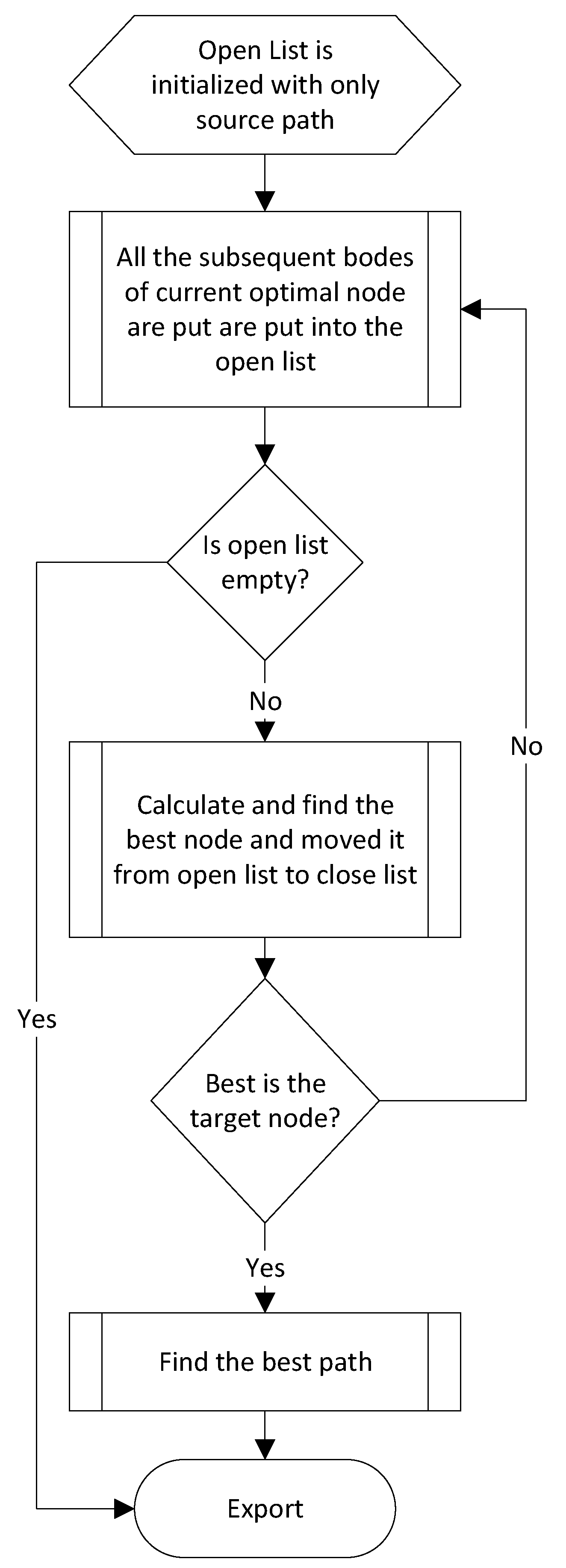
Figure 1.
Flowchart of the improved Dijkstra algorithm used in path planning.

Figure 2.
Exploration of naive random tree selects a node at random from the tree and adds an edge in a random direction [58].
Figure 2.
Exploration of naive random tree selects a node at random from the tree and adds an edge in a random direction [58].

Figure 3.
Exploration of rapidly-exploring random tree are designed to efficiently explore paths in a high-dimensional space [58].
Figure 3.
Exploration of rapidly-exploring random tree are designed to efficiently explore paths in a high-dimensional space [58].

Figure 4.
Exploration of RRT*, which improves on the existing tree by rewiring the tree to form the shortest paths [58].
Figure 4.
Exploration of RRT*, which improves on the existing tree by rewiring the tree to form the shortest paths [58].

Figure 5.
Variants of Firefly algorithm usage, adapted from [87].
Figure 5.
Variants of Firefly algorithm usage, adapted from [87].


Table 1.
Suitability of the Dijkstra algorithm and its variants as classified based upon static and dynamic environmental constraints.
Table 1.
Suitability of the Dijkstra algorithm and its variants as classified based upon static and dynamic environmental constraints.
| Algorithm | Static Constraints | Dynamic Constraints |
|---|---|---|
| Dijkstra | x | |
| Improved Dijkstra | x | |
| Multi-layer dictionary | x | x |
| Floyd and Dijkstra | x |
Table 2.
Most Common Types of Heuristic Functions Used In Path Planning Algorithms.
| Function | Equation |
|---|---|
| Euclidean distance | |
| Manhattan distance | |
| Octile distance | max |
Table 3.
Classification of the A* algorithm and its variants based on static and dynamic constraints.
Table 3.
Classification of the A* algorithm and its variants based on static and dynamic constraints.
| Algorithm | Static Constraints | Dynamic Constraints |
|---|---|---|
| A* | x | |
| Hierarchical A* | x | |
| Improved Hierarchical A* | x | |
| Hybrid A* | x | |
| Guided Hybrid A* | x | |
| A* with equal step sampling | x | |
| Diagonal A* | x | |
| A* with smart heuristics | x | |
| Lifelong Planning A* | x | x |
Table 4.
Summary of D* and its variants.
| Algorithm | Static Constraints | Dynamic Constraints |
|---|---|---|
| D* | x | |
| D* Lite | x | |
| Enhanced D* Lite | x | |
| Field D* | x |
Table 5.
Classification of the RRT algorithm and its variants based on static and dynamic constraints.
Table 5.
Classification of the RRT algorithm and its variants based on static and dynamic constraints.
| Algorithm | Static Constraints | Dynamic Constraints |
|---|---|---|
| RRT | x | |
| RRT Connect | x | |
| Sensor-based Random Tree | x | |
| RRT* | x |
Table 6.
Classification of the ant colony algorithm and its variants based on static and dynamic constraints.
Table 6.
Classification of the ant colony algorithm and its variants based on static and dynamic constraints.
| Algorithm | Static Constraints | Dynamic Constraints |
|---|---|---|
| Ant Colony Optimization | x | |
| Slime mold based optimization | x | x |
| Improved ant colony optimization | x | |
| Adaptive ant colony | x | |
| Enhanced Ant Colony Algorithm | x | |
| Bidirectional ant colony | x |
Table 7.
Classification of the Firefly algorithm and its variants based on static and dynamic constraints.
Table 7.
Classification of the Firefly algorithm and its variants based on static and dynamic constraints.
| Algorithm | Static Constraints | Dynamic Constraints |
|---|---|---|
| Firefly | x | |
| Adaptive Firefly | x | |
| Developed Firefly | x | |
| Modified Firefly | x |
Publisher’s Note: MDPI stays neutral with regard to jurisdictional claims in published maps and institutional affiliations. |
© 2021 by the authors. Licensee MDPI, Basel, Switzerland. This article is an open access article distributed under the terms and conditions of the Creative Commons Attribution (CC BY) license (https://creativecommons.org/licenses/by/4.0/).
Share and Cite
MDPI and ACS Style
Karur, K.; Sharma, N.; Dharmatti, C.; Siegel, J.E. A Survey of Path Planning Algorithms for Mobile Robots. Vehicles 2021, 3, 448-468. https://0-doi-org.brum.beds.ac.uk/10.3390/vehicles3030027
AMA Style
Karur K, Sharma N, Dharmatti C, Siegel JE. A Survey of Path Planning Algorithms for Mobile Robots. Vehicles. 2021; 3(3):448-468. https://0-doi-org.brum.beds.ac.uk/10.3390/vehicles3030027
Chicago/Turabian StyleKarur, Karthik, Nitin Sharma, Chinmay Dharmatti, and Joshua E. Siegel. 2021. "A Survey of Path Planning Algorithms for Mobile Robots" Vehicles 3, no. 3: 448-468. https://0-doi-org.brum.beds.ac.uk/10.3390/vehicles3030027