Machine Learning-Based Control for Fuel Cell Hybrid Buses: From Average Load Power Prediction to Energy Management

Abstract

In this work, a machine learning-based energy management system is developed using a long short-term memory (LSTM) network for fuel cell hybrid buses. The neural network implicitly learns the complex relationship between various factors and the optimal power control from massive data. The selection of the neural network inputs is inspired by the adaptive Pontryagin’s minimum principle (APMP) strategy. Since an estimated value of the global average fuel cell power is required in the machine learning-based energy management strategy (EMS), some global features of driving cycles are extracted and then applied in a feedforward neural network to predict the average fuel cell power appropriately. The effectiveness of the machine learning-based energy management, with the integration of the mechanism of estimating the average fuel cell power based on the forward neural network, is tested under two different driving cycles from the training environment, with comparisons to a commercially used rule-based strategy. Based on the simulation results, the learning-based strategy outperforms the rule-based strategy regarding the charge-sustaining mode conditions and fuel economy. Moreover, compared to the best offline hydrogen consumption, the machine learning-based strategy consumed 0.58% and 0.36% more than the best offline results for both driving cycles. In contrast, the rule-based strategy consumed 1.80% and 0.96% more than optimal offline results for the two driving cycles, respectively. Finally, simulations under battery and fuel cell aging conditions show that the fuel economy of the machine learning-based strategy experiences no performance degradation under components aging compared to offline strategies.

1. Introduction

1.1. Background

Due to the cost problem, the market of passenger vehicles using renewable energy is dominated by full battery electric vehicles instead of fuel cell hybrid vehicles [1]. However, in railway transportation, medium and long-range aircraft, and heavy-duty commercial vehicles, the hybrid power system consisting of fuel cells and batteries is promising due to the limited battery energy density [2,3]. In 2017, the world’s first fuel cell hybrid train began its service in Germany, provided by the company Alstom [4]. Siemens is also working with Deutsche Bahn to test the fuel cell hybrid trains, and the train will begin passenger service between Tübingen, Horb and Pforzheim in 2024 [5]. Compared to fuel cell trains and airplanes, the fuel cell hybrid bus on the street is more often seen. Regionalverkehr Köln GmbH (RVK) operates 35 fuel cell buses, and no company in Europe currently has more fuel cell buses in operation [6]. Furthermore, the RVK receives funding notification for 108 hydrogen-powered fuel cell hybrid buses [7].

Due to the constraints on the change rate of the output power of the fuel cell system and the demand for regenerative braking, another battery system is often applied to provide and absorb high dynamic power. As a result, the fuel cell system’s rated power is scaled down to the average power level. The battery system’s rated power is oriented to the peak power during acceleration and regenerative braking phases. The power distribution between batteries and fuel cells can be utilized to save hydrogen consumption, considering various constraints on components. In the following part, the state-of-the-art energy management for fuel cell hybrid vehicles will be given, and insights based on the authors’ research experience will be shared.

1.2. Literature Survey

Many researchers have studied the energy management for fuel cell hybrid vehicles. Thereby, some good review works can be found in [8,9], and thus a comprehensive review of energy management is not the goal of this work here. Instead, a literature study with a combination of the authors’ research experience will be given.

For fuel cell hybrid vehicles without an extra charger, the hybrid vehicles work in the charge-sustaining mode. In this case, the electrical energy provided by the fuel cell system covers the load energy and the ohmic losses in the battery system. According to the energy balance, the average fuel cell power equals the sum of the average load power and the average battery loss power. The driving cycles primarily determine the average load power, and the energy management does not influence it. In contrast, energy management determines the power distribution between fuel cells and batteries, and then the battery current and the state-of-charge (SoC) trajectories will be directly influenced. Since the battery power losses depend on the battery current and inner resistance, which is strongly dependent on the SoC, it can be concluded that energy management strongly influences the average battery losses. Therefore, two aspects must be considered when designing energy management strategies to reduce hydrogen consumption. On the one side, the fuel cell system must be operated in the high-efficiency range; On the other side, the battery losses must be reduced.

Regarding the first aspect, many works claim to have developed various rules with hyper-parameters to enable the fuel cell system to work within its high-efficiency range. However, the high-efficiency range is not well understood in literature because the high-efficiency range is intrinsically varying and depends on the load conditions. For example, although the fuel cell system has its maximal efficiency in the part-load range, it is not reasonable to operate the fuel cells in the part-load range if the average load lies far higher than the part-load range. The reason lies in the constraint of a charge-sustaining operational mode. Therefore, based on the concept that the high-efficiency range of a fuel cell system varies, a rule-based strategy utilizing the average fuel cell power is proposed by the authors in [10]. The concept of the average fuel cell power utilizes convexity in the specific consumption curve of fuel cell systems. The convexity in this case means that the efficiency at the average fuel cell power is larger than the average efficiency of the fuel cell power trajectory. Further information about utilizing convexity in energy management for fuel cell hybrid vehicles can be found in [10].

Regarding the second aspect of reducing the ohmic battery losses, a compromise of distributing dynamic power during acceleration and regenerative braking between fuel cells and batteries has to be found. For example, suppose the fuel cell power is strictly kept at the average load power value. Then, the battery system must afford the full dynamic power, which is the difference between the transient load power and the average load power. As a result, the battery charge and discharge currents are large, and the corresponding battery power losses also increase. Therefore, to reduce the ohmic battery losses, the fuel cell system is suggested to share some dynamic power as long as the fuel cell power dynamic constraints are not violated. Then, the next task is to find a compromise in distributing the dynamic power between fuel cells and batteries. On the one hand, the battery losses are reduced, and on the other hand, the fuel cell system’s operation is not far from the average load power mentioned before. The authors developed an adaptive Pontryagin’s minimum principle (APMP)-based strategy in [11,12] for reasonable dynamic power distribution. An analytical formula for calculating the costate defined in the optimal control theory is derived and validated. It is worth mentioning that the equivalent consumption minimization strategy (ECMS) is mathematically the same as the APMP because the equivalent factor in ECMS is linked to the costate in the APMP. However, it is suggested by the authors to use the APMP instead of ECMS because the ECMS is a simplified version of the APMP, which has poorer performance compared to the APMP. Using the analytical formula to estimate the costate in APMP, the fuel cell power is slightly higher than the average fuel cell power during acceleration phases and slightly lower than the average fuel cell power during regenerative braking. However, the fuel cell power is almost equal to the average power during the rest driving time. Summarily, the fuel cell system under the APMP strategy is operated around its average power to enable high-efficiency operation on one side. On the other side, the fuel cell power oscillates around its mean value during acceleration and regenerative braking to reduce the battery current, reducing battery ohmic losses. Therefore, the developed APMP-strategy represents the state-of-the-art energy management for fuel cell hybrid vehicles.

Nevertheless, there is still room for improvement regarding average fuel cell power estimation. In [10], the history information, including load power, battery ohmic losses and gradient, is used to estimate the fuel cell power. The deviation in estimating the average fuel cell power decreases with more history information collected. However, there is not enough history information at the beginning of driving cycles. Therefore, the method provided in [10] cannot estimate the average fuel cell power in the beginning phases of driving cycles. In order to handle this problem, a feedforward neural network will be utilized to estimate the average fuel cell power based on features of driving cycles such as average speed along the routes, average gradient, average number of stops along the trip and average total weight of the hybrid vehicles. Since average values of features are used instead of time series data, it is much less challenging to realize the average power estimation. Since the feedforward neural network will be used in this work, many driving cycles with different values in the average speed, gradients, number of stops, and weight must be prepared. One way to collect training data for the neural network is to collect real driving cycles, which is time-consuming and challenging to collect enough driving cycles, since more than a thousand driving cycles is required for training networks. Therefore, data extension methods are applied to generate enough driving cycles with different features in this work based on some real driving cycles.

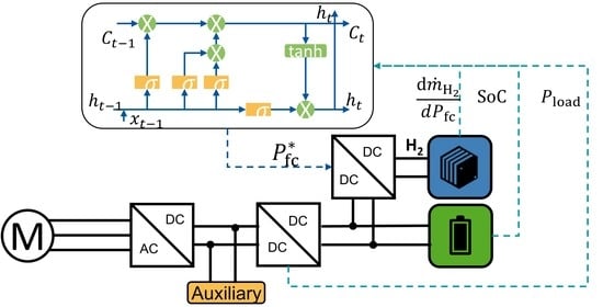
Besides the improvement in estimating the average fuel cell power, reducing battery ohmic losses can be done to have a more energy-efficient energy management strategy than the APMP-based strategy. Since the ohmic battery losses are dependent not only on the battery current but also on the varying inner resistance, it is suggested to have a small battery current and low inner resistance. The battery current is reduced under the APMP-based strategy because the fuel cell power shares part of the dynamic power during vehicle acceleration. Besides that, keeping the battery inner resistance low is another way to improve the fuel economy, which can be understood as follows. As the fuel cell vehicles work in the charge-sustaining mode, the start and ending SoC of the battery system must be equal. However, the number of SoC trajectories having the same start and end SoC values is endless. Thereby, there are two typical types of trajectories. One type of the SoC trajectory can first go down, then go up, and finally reach the same value as the beginning value. In contrast, the second type of the SoC trajectory can first go up, then go down, and finally reach the same value as the beginning. After comparison, in the second type of SoC trajectory, the SoC average value is higher than that in the first type of SoC trajectory, which leads to lower inner battery resistance and fewer ohmic battery losses. Furthermore, an SoC trajectory with higher average values results in a higher average open-circuit voltage, which reduces battery currents if the same battery power is required. In this way, the ohmic battery losses are reduced because of the lower inner resistance and the lower battery current for the same amount of battery power. From this aspect, the fuel cell power must be decreased tendentially along with the driving cycles. At the beginning of the driving cycles, the fuel cell power can be increased above the estimated average fuel cell power even in the phase of cruising, which leads to a tendential going up of the SoC trajectory. Then, along with the driving cycles, the fuel cell power is decreased below the estimated average value even in the phase of cruising to let the SoC trajectory come down, which is necessary for the charge-sustaining mode. This phenomenon of the SoC trajectory first going up and then coming down is also found in the offline PMP results. Thereby, the costate amplitude at the beginning of driving cycles is larger than that at the end. However, the formula in the so-far developed APMP-based strategy in [11] calculates the same costate values for the driving cycles’ initial and end time points. Therefore, reducing the battery inner resistance by increasing fuel cell power in the beginning phases of driving cycles to above-average values to improve fuel economy is not included in the APMP strategy. In this work, this kind of time effect of enlarging fuel cell power at the beginning of driving cycles and decreasing along the trip will be considered using an LSTM network. Since machine learning is used in this work, several works about using machine learning will be introduced in the following parts.

With machine learning technology evolved, machine learning-based strategies attract more and more attention in energy management. They can be divided into unsupervised learning, supervised learning, and reinforcement learning-based strategies. Unsupervised learning is not actively used and is mainly used to classify driving profiles through clustering. Reinforcement learning is a learning process of the policy principle by utilizing the interaction between agents and the environment under the pre-definition of a reward function. The advantage of reinforcement learning is that it can learn long-term accumulated rewards. However, for hybrid vehicles, its most significant drawback lies in the limited transferability of the trained control models. This limitation lies in that the data used in training can not cover all the driving situations. Moreover, the control policy is updated based on the maximization of accumulated reward function during training after each time step. Furthermore, various goals have to be considered to define the reward function, which leads to a lack of physical meanings. For example, different factors, including fuel consumption, component aging, and charge sustaining, are integrated into the reward function using weighting coefficients. However, the coefficients lack physical meaning, whose tuning is challenging without a reasonable universal solution for all changeable driving conditions. Due to the problems in using reinforcement learning, this method will not be used in this work.

Supervised learning is active in research, including the forward and recurrent neural networks. The forward neural network aims to identify the nonlinear relationship between the inputs and the output. However, the forward neural network cannot capture the sequential information needed to process sequential data in the input data, which the recurrent neural network can do. One of the recurrent neural networks is the so-called long short-term memory (LSTM) network, which is good at identifying the time effects included in the input variables. Due to the advantages of different neural networks, there are two common applications for hybrid vehicles. The first application is to use machine learning-based models to predict future driving information, e.g. velocity profiles [13,14,15], roadway types [16], traffic congestion levels [17] and driver’s driving styles [18]. In [13], the vehicle speed is first predicted through a Markov decision process, then model predictive control (MPC) utilizes the predicted speed trajectory. In [19], the future 10-second velocity profile is predicted by an LSTM network, and the predicted velocity is then used as an input for the dynamic programming algorithm. In [18], the concept of driving pattern recognition is used. In each representative driving pattern, control parameters of a parallel hybrid electric vehicle are optimized offline. First, the driving pattern is recognized in the real-time application, and then the driving control algorithm is switched to the corresponding one. Summarily, to our best knowledge, an estimation of the average power based on machine learning has not been found, and this work will fill this gap.

The second application area of machine learning in fuel cell hybrid vehicles is to develop energy management using data generated by the offline optimal control strategy. In [16], besides the roadway type and traffic congestion level predictor, another neural network is used to determine battery power and engine rotational speed with traffic congestion and driving trends as inputs. The training data are obtained offline by dynamic programming. In [20], a neural network is used to predict the equivalent factor in the ECMS. First, three input features are chosen, including the load power, battery SoC and the ratio of distance traveled to the total distance. Then, the offline results of ECMS construct the training data, and the neural network is trained to predict the current equivalent factor using instantaneous load power, battery SoC and the distance ratio. In [21], several neural networks are applied for driving environment prediction and optimal power control. Summarily, supervised learning is promising for developing energy management strategies. However, the input variables of the neural network, as found in literature, are not chosen physically, which leads to the trained network’s lack of transferability to different driving cycles from the training environment. Therefore, to fill this gap, the neural network’s input variables in this work are chosen physically, enabling the trained model to have powerful adaptivity.

1.3. Main Work

Following major contributions are included in this work:

• A feedforward neural network is applied to predict the average fuel cell power, which can be further used in the machine learning-based strategy.
• Data extension methods generate enough training data so that collecting lots of real driving cycles is not required.
• An LSTM network-based energy management is developed to consider the so-called time effect to improve fuel economy further, compared to the APMP-based strategy which represents the state-of-the-art.
• The input variables of the LSTM network are chosen based on the physical correlation between them and the output fuel cell power so that the trained network works well under different driving cycles from the training environment.
• The robustness of the LSTM network-based energy management against fuel cell and battery aging regarding fuel economy is verified based on simulations.

1.4. Paper Organization

The system modeling required for analyzing the fuel economy is shortly introduced in Section 2. In Section 3, a feedforward neural network is constructed to support the estimation of average fuel cell power. In Section 4, an energy management strategy using the LSTM network is developed and verified by using simulations. Finally, a short conclusion will be given in Section 5.

2. Driveline

The configuration of the fuel cell hybrid bus is shown in Figure 1. The required power is offered by the fuel cell and battery system together. The fuel cell system actively offers the average load power with low dynamic, and the battery system offers the remaining power with high dynamic. The total power flows through DC/DC and inverters into the electrical machine, converted into mechanical power. Finally, the torque provided by the electrical machine is transferred through the gears and axle into the wheels, and, therefore, the vehicle moves forward. When braking, the electrical machine switches to generator mode, and the power flows in the reverse direction. Thus, the battery system becomes charged. It has to be mentioned that the power demand for the auxiliary devices, including air condition, is assumed constant in this work.

2.1. Fuel Cell System

A fuel cell system provides electrical energy resulting from a chemical reaction between the supplied fuels. Accurately modeling the entire fuel cell system in multiple domains is complicated. Therefore, using a quasi-static fuel cell model is general in energy management applications. In this model, the hydrogen consumption rate depends on the fuel cell power. The relationship between hydrogen consumption rate and power is shown in Figure 2, where the convexity is also identified because the line segment between any two points is higher than the value of the function between these two points. The maximum fuel cell power is 85 kW.

2.2. Lithium-Ion Battery System

Since the fuel cells can only deliver a maximum power of 85 kW, a battery system is also applied so that the peak power demand during acceleration can be met. The use of the battery also enables regenerative braking. The SoC, which is the ratio of the amount of charge stored in the battery to the total amount of charge that the battery can store, is defined as follows:

$$SoC=\frac{Q\left(t\right)}{Q_{\mathrm{norm}}},$$

(1)

where $Q_{\mathrm{norm}}$ is the total rated capacity and $Q\left(t\right)$ is the currently stored amount of charge. The dynamic of the battery SoC is determined by:

$$\dot{x}\left(t\right)=\dot{SoC}\left(t\right)=-\frac{I\left(t\right)}{Q_{\mathrm{norm}}},$$

(2)

where the $I\left(t\right)$ is the battery discharge current. The internal resistance $R_0$ and open-circuit voltage $V_{\mathrm{oc}}$ of a lithium-ion high-performance cell are dependent on the SoC and the dependency is described in Figure 3. The battery system has three parallel branches, and each branch has 227 cells connected in serials with a nominal voltage of 584 V and a maximal power of 175 kW.

2.3. Electrical Machines

The electrical machine is modeled by using look-up tables. The torque demand M and the rotational speed $n_{\mathrm{Motor}}$ are inputs. Four look-up tables are used here: power losses $P_{\mathrm{loss}}(M,n_{\mathrm{Motor}})$, motor current $I(M,n_{\mathrm{Motor}})$ motor voltage $U(M,n_{\mathrm{Motor}})$, and power factor $cos\varphi (M,n_{\mathrm{Motor}})$.

The total electrical power of the electric machine is calculated as follows:

$$P_{\mathrm{el},\mathrm{motor}}=P_{\mathrm{loss},\mathrm{motor}}+P_{\mathrm{mech}}=P_{\mathrm{loss},\mathrm{motor}}+\frac{2\pi n_{\mathrm{Motor}}·M}{60},$$

(3)

where $P_{\mathrm{mech}}$ is the demanded mechanical power. Since the power loss $P_{\mathrm{loss},\mathrm{motor}}$ is always positive, $P_{\mathrm{el},\mathrm{motor}}$ is larger than $P_{\mathrm{mech}}$ in motor operation and $P_{\mathrm{el},\mathrm{motor}}$ is smaller than $P_{\mathrm{mech}}$ in generator operation regarding amplitude.

The power losses in inverters and DC/DC converters are also modeled by using look-up tables, which are simulated by using the software Plecs. The look-up table for modeling inverter losses requires inputs, such as motor current, motor voltage, power factors, and rotational speed. The look-up table for modeling the DC/DC converter requires inputs, such as the battery voltage and power demand on the DC-link. Detailed modeling descriptions can be found in [11].

2.4. Driving Cycles

Four bus routes are collected, named line 1 to line 4 in this work. Line 1 is the route on which the novel van Hool A330 FC fuel cell bus has been operated since 2020. The bus runs between Bensberg Central Bus Station and Cologne/Bonn Airport. Line 2 locates in Interlaken, Switzerland. Line 3 is located in the German city Aachen, and line 4 is in the Chinese city Beijing.

The relative elevations along the routes compared to their start positions are displayed in Figure 4. Line 2 is the most aggressive compared to other lines, which presents a more significant challenge for energy management because the power demand dynamic is relatively large. On the other hand, the gradient change of line 4 is small and, therefore, is ignored.

It is worth mentioning that the driving cycles above are not directly given. Instead, a two-dimensional dynamic programming method proposed in [22] is used to generate velocity profiles using available information, such as timetables, altitude, and velocity limits along the routes. The stopping time between two sub-driving cycles is randomly generated according to Gaussian distribution. These lines have the same average stopping time at stations, which is predefined in advance. The generated velocity profiles are shown in Figure 5. In the following, lines 1 and 2 will be used to construct the training and validation data, respectively. Training is used to update parameters of the neural work, and validation is utilized to determine if the phenomenon of overfitting happens and then choose the model with the best performance on the validation dataset. Lines 3 and 4 will be used as testing data in the online simulation environment. Testing is applied to evaluate the performance of the trained model under a different environment from training data.

3. Machine Learning-Based Average Power Prediction

It has been shown that global average fuel cell power is essential for energy management in [10,11]. The concept of operating the fuel cell system close to the average load power has been used to develop a rule-based strategy in [10] and the APMP in [11], respectively. In this work, the global fuel cell power will also be utilized for the machine learning-based EMS in the next section. The global average fuel cell power cannot be known in advance in the real-time application, and it has to be estimated on-the-fly. In [10,11], a history information-based method is proposed to estimate the average fuel cell power. However, due to the limited amount of historical information at the start of driving cycles, a large deviation usually occurs at the beginning. To mitigate this deviation, we propose to use some global features to complement the prediction. These global features contain helpful information about driving cycles to be driven and are used in a feedforward neural network to predict the global average fuel cell power. This section is organized as follows. First, the previous work’s estimation method of the global average fuel cell power is reviewed, including the average power’s definition, meaning, and estimation. Second, an estimation algorithm using a feedforward neural network is presented. Finally, the experiments and estimation results are presented.

3.1. Review of the Concept of Estimating the Average Fuel Cell Power

The average fuel cell power of the journey with total travel time T is defined as:

$${\overline{P}}_{\mathrm{fc}}=\frac{{\int }_{t=0}^T{P}_{\mathrm{fc}}\left(t\right)dt}{T}.$$

(4)

According to the principle of energy conservation, the following equation related to average fuel cell power, battery power, load power, and battery power losses can be derived:

$${\overline{P}}_{\mathrm{fc}}={\overline{P}}_{\mathrm{load}}+{\overline{P}}_{\mathrm{bat},\mathrm{loss}}+\frac{\Delta E_{\mathrm{bat}}}{T},$$

(5)

where ${\overline{P}}_{\mathrm{load}}$ represents the average load power, ${\overline{P}}_{\mathrm{bat},\mathrm{loss}}$ represents the average battery loss, and $\Delta E_{\mathrm{bat}}$ represents the energy difference corresponding to SoC variations of the battery system. Because the fuel cell hybrid bus is operated in the charge-sustaining mode, $\Delta E_{\mathrm{bat}}$ equals zero. Therefore, the average fuel cell power is determined by the load power and the battery losses as follows:

$${\overline{P}}_{\mathrm{fc}}=\frac{{\int }_0^T{P}_{\mathrm{load}}\left(t\right)+P_{\mathrm{bat},\mathrm{loss}}\left(t\right)dt}{T}.$$

(6)

From the results of dynamic programming in [23] and the offline Pontryagin’s minimum principle (PMP) in [11], it can be seen that the fuel cell system works around its global average power. The reason lies in the convexity of the specific consumption curves of fuel cell systems. Based on this observation, an adaptive rule-based strategy and an APMP-based strategy are proposed in [10,11], respectively. Both of them have achieved better results than previous work. It helps the fuel economy and the fulfillment of the charge-sustaining-mode condition. So far, the importance of the average fuel cell power is verified.

In order to make use of the global average fuel cell power, a history-based method was proposed in [10,11] to predict the average fuel cell power, which utilized the history power information. It is formulated as follows:

$${\overline{P}}_{\mathrm{fc}}\left(t\right)=\frac{{\int }_0^t{P}_{\mathrm{load}}\left(\tau \right)+P_{\mathrm{bat},\mathrm{loss}}\left(\tau \right)d\tau }{t}.$$

(7)

As the fuel cell power is overestimated in the acceleration stage, the updated instance of the estimation is chosen as the departure of the vehicle, as shown in Figure 6. In addition, the gradient force leads to considerable differences in load power between uphill and downhill, i.e., if the vehicle first goes uphill and then downhill, the average load power will be overestimated and vice versa. Therefore, the instantaneous gradient is replaced by the average gradient when calculating the load power. For a more detailed description, please refer to [10,11].

This method is simple to implement because only the gradient information, the history load power, and battery losses are needed, and they are easy to collect. Moreover, it can achieve high accuracy under enough historical information. However, as this method is mainly based on historical information, the estimation is not accurate at the beginning of the journey because the historical information is insufficient.

3.2. Average Power Estimation with Global Features

There is some pre-known information about the entire driving cycle for buses, such as the total distance and number of bus stops. If congestion is not considered, the total travel time is also known in advance. These pieces of information are helpful because they strongly influence the average power demand of the driving cycle. In the initial stage of the journey, as the historical information is quite limited, it is believed that these pieces of information are more helpful than the limited historical information in predicting the average power. In order to improve the estimation accuracy in the initial phase, some global features of driving cycles will be extracted to complement the average power estimation. These features must strongly influence average load power and battery losses. They are also expected to be collected conveniently and accurately on-the-fly. In this work, some intuitive features are first selected and then further validated by experiments, and they are:

• Average speed $\overline{v}=\frac{S}{T}$, where S is the total distance of the driving cycle and T is the total travel time.
• Average gradient along the route $\overline{g}=\frac{1}{S}{\int }_{s=0}^S|tan\left(\theta \right)|d\left(s\right)$, where S is the total distance of a driving cycle, $\theta$ is the slop angle along the route.
• Average distance between two nearby stops $\overline{d}=\frac{S}{N}$, where N is the number of stops. As the vehicle can stop because of traffic lights and congestion, the "stop" here means the point where the speed is zero.
• Average mass $\overline{m}=m_{\mathrm{bus}}+\frac{1}{T}{\int }_0^T{m}_{\mathrm{pass}}\left(t\right)dt$, where $m_{\mathrm{bus}}$ and $m_{\mathrm{pass}}$ represent the vehicle mass and total passengers mass, respectively.

In order to test the effect of the selected features on the average power, some artificial driving cycles are created by using data extension methods. In addition, several driving cycles are created to have other features be the same except for the feature to be tested during testing a feature.

3.2.1. Influence of Average Speed on the Mean Power

In order to test the influence of the average speed on the average power, three driving cycles with different average speeds are used. Part of the driving cycles and the result are shown in Figure 7. It can be seen that the average load power and the average speed are positively correlated. Therefore, the average speed value strongly influences the average load power level.

3.2.2. Influence of Average Gradient on the Mean Power

In order to test the influence of the average gradient on the average power, three driving cycles with different average gradients are used. These journeys have the same features except for the gradients. The result is shown in Figure 8. Similar to the average speed, the mean load power and the average gradients are also positively correlated.

3.2.3. Influence of Average Distance between Nearby Stops on the Mean Power

More stops for a typical driving cycle means more accelerations and brake phases. The used driving cycles for feature tests and the corresponding results are in Figure 9. From the result, it can be seen that a larger average distance between stops leads to less mean power.

3.2.4. Influence of Average Weight on the Mean Power

In order to test the influence of average weight on the average power, the driving cycle with different averaged passengers’ total weight is used, keeping other factors the same. In this work, the weight of each passenger is set to be 70 kg, and the number of passengers is variable from time to time. However, the mean values of the passenger number remain constant throughout the journey. We also tested the effect of variance of weight distributions on the average power. The passengers’ number is created with Gaussian distribution, with the same mean value but different variance.

The results are shown in Figure 10. It can be seen that the mean power increases with the increase in the average passenger number. Therefore, the total weight strongly influences the mean power. However, the average load power remains almost the same under different variances of Gaussian distribution.

In addition to the features mentioned above, the vehicle acceleration is intuitively closely relevant to the load power. Therefore, we have also conducted simulations to test its influence on the average power. For that purpose, driving cycles with different accelerations are used, while the other features remain the same. It has to be noted that the average acceleration is only calculated in the acceleration and brake phases, i.e., the driving phase, when the speed is almost constant, is excluded. Part of the driving cycles with different acceleration and results are shown in Figure 11. The results show that the difference in the mean power under the different accelerations is minimal, and, also, there is no clear correlation between the mean power and the acceleration. Therefore, the acceleration is not chosen to be a feature for estimating the average power.

In the real-time application, the total distance is almost fixed for a pre-defined route, and the travel time of a bus line is known in advance if congestion is not taken into account. Therefore, the average speed can be known in advance. Furthermore, the average gradient is also known since the terrain information is also available. Unfortunately, the number of stops cannot be known in advance due to congestion and traffic lights. However, with the development of intelligent transportation systems, predicting future locations can be accurate. Therefore, the number of stops is assumed to be known in advance in this work. As for the passengers’ number, it is generally assumed that it follows a Poisson distribution. Additionally, the average weight of each passenger is available. Then, the total weight of the passengers can be estimated on-the-fly and, therefore, the average weight can also be estimated.

After determining the representative features, the next question is how to use them to predict the average power. A straightforward option is to build a look-up table. However, a multi-dimensional look-up table is enormous and requires a lot of storage space. In addition, as the global features do not include the driving details and only represent a tendency, they are not one-to-one mapping to the average fuel cell power. Therefore, a look-up table is not an optimal option. Another simple, modern, and elegant option is to use a neural network, which is well suited for approximating complex functions. Moreover, it can achieve high accuracy with quite limited parameters. Therefore, the neural network is chosen for the mean power prediction.

The feedforward neural network is chosen as the model architecture because the prediction target has a global feature, and the inputs are also average values instead of time-series data. The inputs are the following features, including average speed, average gradient, average distance, and average weight:

$$\mathit{x}={[\overline{v},\overline{g},\overline{d},\overline{m}]}^T.$$

(8)

The task is to train a neural network to predict the mean power of a journey. Thus, the target is the actual mean power, denoted as y, a scalar. The output of the neural network is the estimated mean power, denoted $\widehat{y}$. Given the prediction and the target, we can calculate the loss, e.g., using absolute error loss or square error loss, and update the parameters using a gradient descent algorithm.

3.3. Training of the Feedforward Neural Network

3.3.1. Driving Cycles Expansion

In order to train a neural network, the quantity and quality of data are extremely important because the model learns knowledge from the data. Therefore, the data should be extensive, rich, and diverse, and the data samples should be of high quality. Without enough data, sufficient learning is not possible. Furthermore, sufficient data is also required for reliable evaluation of the model. In our case, the driving cycles must cover a variety of average speeds, gradients, and distances between two stops. Unfortunately, collecting so many realistic driving cycles with enough diversity is time-consuming. Therefore, some data extension methods are applied to increase the variety of the existing driving cycles.

Average Speed

The average speed is expanded by multiplying a ratio from 0.9 to 1.1 with an interval of 0.05, i.e., 0.9, 0.95, 1.0, 1.05, and 1.1. Correspondingly, the driving time is adjusted to keep the total distance unchanged. For example, the average speed of the original bus line 1, as shown in Figure 5a, is 8.66 m/s, so the expanded training data covers a range from 7.74 m/s to 9.46 m/s (for simplicity, stopping time is not considered). This range is sufficient to check the effectiveness of the algorithm. A larger average speed range can be created to cover a more extensive search range if necessary.

Average Gradient

Similar to expanding the average speed range, the average gradient is also expanded by multiplying it by a ratio to the original gradient.

Average Distance between Nearby Stops

In order to achieve a greater variety of average distance between two stops, the number of stops and their positions are adjusted. The process of expanding the number of driving cycles with a different average distance between two nearby stops consists of four steps:

• Choose an average distance $\overline{d}$ between two stops.
• Calculate the number of stops, $N_{\mathrm{stops}}=\frac{S}{\overline{d}}$, where S is the total distance. The $N_{\mathrm{stops}}$ will be rounded to the closest integer number, if the division result is not an integer. In that case, the average distance $\overline{d}$ will be recalculated based on the integer number of stops.
• The position of each stop is randomly set within a reasonable distance range between two stops.
• Create new driving cycles using the two-dimensional dynamic programming method.

An example is illustrated in Figure 12. Assume the total distance is 5 km. There are five stops during the journey. Then, the initial average distance between two nearby stops is 1000 m. If we want to have an average distance of 1250 m, the new number of stops is four. As the first and last stop positions are fixed, the other three stops are randomly set between the first and the last stop, whereby the distance between two stops is within a reasonable range, e.g., from 500 m to 1500 m.

Average Weight

In order to cover a variety of different average weights, different passengers’ numbers are used. They vary from 10 to 50, with an interval of 10. Summarily, bus line 1 is expanded to more than 4000 driving cycles, and bus line 2 is expanded to more than 1000 driving cycles. However, bus lines 3 and 4 are not expanded, and they are used for the final test in online simulations. The results of the data expansion methods are listed in

Table 1. Range of features of the driving cycles 1 and 2 after data expansion.

Features	Bus Line 1	Bus Line 2
average speed	(7.39 m/s, 9.48 m/s)	(7.88 m/s, 9.17 m/s)
average gradient	(0, 0.055)	(0, 0.0335)
average distance	(951 m, 2075 m)	(1000 m, 1250 m)
average weight	(14.3 t, 17.8 t)	(14.3 t, 17.1 t)

.

3.3.2. Configurations

As mentioned earlier, the training data are constructed based on the expanded driving cycle of line 1, and the validation data are constructed using the driving cycle of line 2. The corresponding ranges of features are listed in Table 1. Min–max normalization is applied to both the inputs and the target. The neural network has one hidden layer with a size of 25 and an output layer. ReLU (Rectified Linear Unit [24]) is used as the activation function. The loss function is the mean square error (MSE), and the L2 regularization method is used to avoid overfitting. The learning rate is 0.001 and remains constant throughout the training process. The Adam optimizer with default hyper-parameters is used. In addition, a batch gradient descent with a batch size of 50 is used.

3.3.3. Evaluation Metrics in Network Training

In order to measure the performance of the model, various metrics can be used, and one is the mean square error loss. However, this is not very intuitive, and people cannot obtain an immediate sense of the performance. Therefore, another metric is used, which is called relative difference here and denoted as ${\Delta }_{\mathrm{rel}}$. It is the relative difference between a prediction y to its target $\widehat{y}$. Given N predictions and the corresponding targets, it is calculated as follows:

$${\Delta }_{\mathrm{rel}}=\frac{{\sum }_{i=1}^N{\displaystyle \frac{|{\widehat{y}}_i-y_i|}{y_i}}}{N}.$$

(9)

3.3.4. Results and Ablation Study

The best results after training are displayed in

Table 2. Training and validation results.

Training Loss in kW${}^2$	Validation Loss in kW${}^2$	${\mathbf{\Delta }}_{\mathbf{ref}}$
0.0001788	0.0001794	1.2%

,

where the training loss is the loss on the training data, the validation loss is the loss on the validation data, and ${\Delta }_{\mathrm{ref}}$ is the relative difference between the predicted mean power and the actual mean power on the validation dataset, as defined in (9). As the training loss and the validation loss are very similar, it is concluded that no overfitting occurs. The relative difference between the predictions and the targets is relatively small, which validates the effectiveness of the neural network.

Ablation experiments are performed to investigate the influence of some setups of the neural network. The learning rates of the following experiments are all tuned to obtain good results. First, the type of normalization is considered. For this purpose, experiments with mean-variance normalization and min–max normalization are performed. The results are shown in

Table 3. Results of ablation studies on different normalization types.

Normalization Type	Training Loss	Validation Loss	$\mathbf{\Delta }$rel
	in kW${}^2$	in kW${}^2$	-
Min–max normalization	0.0001788	0.0001794	1.2%
Min–max normalization (only to inputs)	1.260	1.278	2.9%
Mean-variance normalization	0.001287	0.001968	3.9%

. Since different normalization methods are applied to the target, we cannot directly compare the loss, but we can compare the relative difference between the prediction and the target. It can be seen that applying the min–max normalization to the inputs and the target gives the best results. On the other hand, if we apply the min–max normalization only to the inputs, we obtain worse results. However, it is still better than the mean-variance normalization. The reason for the worse performance under the mean-variance normalization lies in that the original training data inputs have a significant variance, e.g., the average distance has a range from 951 m to 2075 m and variance of 115,602 ${\mathrm{m}}^2$. However, if the mean-variance normalization is applied, all the inputs after normalization cannot be distinguished. So in the following experiments, the min–max normalization is applied to inputs and targets.

Furthermore, we test the influence of the model size, i.e., the number of layers and the size of the hidden layers. The results are shown in

Table 4. Results of ablation studies on different model size.

Model Size		Training Loss in kW${}^2$	Validation Loss in kW${}^2$	$\mathbf{\Delta }$rel
Layers	Hidden Size
1	15	0.000216	0.000262	1.60%
1	25	0.000179	0.000179	1.20%
2	15	0.000212	0.000257	1.40%
2	25	0.000174	0.000195	1.20%

. It can be seen that the models with a hidden layer size of 25 achieve the best results. Since the model with one hidden layer has a smaller model size, it is preferred for real-time applications regarding memory and speed.

3.4. Online Simulation

Once the training process is completed, the model with the best result on the validation set is selected for use in the online simulation environment. The accuracy of the estimated average power by using the neural network-based method is evaluated and compared with the history-based strategy.

As mentioned above, traffic congestion is not considered in this work. Therefore, the total travel time is assumed to be known in advance. As the total distance is fixed, the average speed can be taken as given. The average gradient can also be determined since the entire route is also known. Furthermore, the number of stops because of traffic lights is assumed to be predicted by other means, e.g., an intelligent traffic system. The average distance between two stops is therefore also accurately predictable. Finally, the total number of passengers follows a Poisson distribution, and the average number of passengers is estimated as follows:

$${\overline{m}}_{\mathrm{esti}}=\frac{{\int }_{\tau =0}^{t}m\left(\tau \right)d\tau }{t},$$

(10)

where $m\left(\tau \right)$ is the total weight of the bus and passengers. The estimated average weight ${\overline{m}}_{\mathrm{esti}}$ is only updated at the departure of the bus. So far, the input variables have been obtained, and the mean power can be estimated using the feedforward neural network model.

The machine learning-based model predicts the mean power based on prior knowledge of the driving cycle. Therefore, it is expected to achieve a better result than the history-based strategy in the initial stage. On the contrary, the history-based strategy is more promising for obtaining a better estimation if sufficient history information is given. Therefore, the two methods are combined with a weighting factor $\alpha$ in estimating the mean fuel cell power. Formally, the final estimated mean power is formulated as follows:

$${\overline{P}}_{\mathrm{fc},\mathrm{esti}}=\alpha \left(t\right)·{\overline{P}}_{\mathrm{fc},\mathrm{ml}}+(1-\alpha \left(t\right)){\overline{P}}_{\mathrm{fc},\mathrm{hist}},$$

(11)

where ${\overline{P}}_{\mathrm{fc},\mathrm{ml}}$ is the predicted fuel cell average power based on the machine learning model, ${\overline{P}}_{\mathrm{fc},\mathrm{hist}}$ is the estimation by using the history-based method. A heuristic formula is designed for the weighting factor $\alpha$ dependent on time:

$$\alpha \left(t\right)=\left\{\begin{array}{cc}1\hfill & \frac{t}{T}<{\alpha }_{\mathrm{th}},\hfill \\ 1-\frac{t}{T}\hfill & \mathrm{else}.\hfill \end{array}\right.$$

(12)

The ${\alpha }_{\mathrm{th}}$ denotes the empirical ratio threshold, above which enough history information is collected to estimate the average power accurately. In this work, 0.5 is used for this threshold value ${\alpha }_{\mathrm{th}}$. Although the machine learning model is used combined with the history-based strategy, for simplicity, we still call it a machine learning-based estimating method.

As described in Section 2, another two bus lines, different from the training environment, are used for the online tests. One is line 3 in the German city Aachen with a relatively large average gradient. The second one is line 4 in Beijing in China, whose average gradient is zero. Different average ridership is used for the two lines. It must be noted that a Gaussian distribution is used to approximate the Poisson distribution for reasons of mathematical approximation, and different means and variances in the passenger number are used to model the ridership. Their parameters are summarized in the

Table 5. Characteristics of the driving cycles for online simulation tests.

Features	Bus Line 3	Bus Line 4
average speed	7.4 m/s	8.5 m/s
average distance	1016 m	999 m
average gradient	0.0193	0
ridership	mean/variance	mean/variance
	40/40	30/30

.

The results are as shown in Figure 13.

In line 3, it is evident that the estimated mean power of the history-based strategy has a significant deviation from the global mean power, while the deviation is much smaller for the learning-based strategy. For line 4, the history-based strategy obtained an excellent estimate, as expected, due to the zero gradient and the uniform velocity distribution in bus line 4. Nevertheless, it can be seen that the learning-based strategy still has a slightly lower deviation in the initial phase.

The results show that the learning-based strategy has successfully mitigated the significant deviation problem of the history-based strategy at the beginning of driving cycles.

4. Machine Learning-Based Energy Management

The energy management strategy for fuel cell hybrid buses is crucial and complicated to realize optimum under various constraints. It is almost impossible to consider all the relevant factors explicitly. This section proposes a machine learning-based EMS strategy, which aims to learn the optimal strategy from the data implicitly. This section is structured as follows. First, the choice of the neural network and input variables is explained. After that, the details of the neural network training and the online experiment results are presented. Finally, robustness tests of the machine learning-based strategy against battery and fuel cell aging are performed.

4.1. Choice of the Neural Network and Input Variables

Unlike the last section’s average fuel cell power estimation, a so-called time effect is observed in the fuel cell power trajectory resulting from optimal offline control. The time effect describes the phenomenon that the average fuel cell power at each time stage is not equal to the global value but decreases with time. The time effect is evident when the total travel time becomes longer. Figure 14 illustrates a offline optimal fuel cell power trajectory for a fuel cell hybrid train in [11]. Under this fuel cell power trajectory with decreasing tendency, the SoC can be kept at a relatively higher level than a constant average fuel cell power throughout the journey. The higher level of SoC corresponds to larger battery voltage and lower battery internal resistance. Then, the battery losses will be reduced due to lower battery current and inner resistance for the same amount of battery power.

In order to consider the time effect, the LSTM network, a famous variant of the recurrent neural network, is chosen, which is capable of learning time dependency implicitly. Compared to the LSTM network, other network is not good at learning this kind of time effect.

The APMP algorithm in [11] inspires the choice of the neural network input variables. The APMP algorithm is a local optimization-based strategy where the fuel cell power at each time step is determined by minimizing a Hamiltonian function as follows:

$$H(SoC\left(t\right),P_{\mathrm{fc}}\left(t\right),\lambda \left(t\right),t)={\dot{m}}_{{\mathrm{H}}_2}\left(P_{\mathrm{fc}}\left(t\right)\right)+\lambda \left(t\right)·\dot{SoC}\left(t\right),$$

(13)

where ${\dot{m}}_{{\mathrm{H}}_2}$ is the mass flow of fuel cell system, which depends on the output fuel cell power, $P_{\mathrm{fc}}\left(t\right)$ is the fuel cell power at time step t, and $\lambda \left(t\right)$ is the costate defined in the theory of optimal control. Then, the optimal control variable is found with the following equation:

$$P_{\mathrm{fc}}^{*}\left(t\right)=\underset{P_{\mathrm{fc}}}{argmin}H(SoC\left(t\right),P_{\mathrm{fc}}\left(t\right),\lambda \left(t\right),t).$$

(14)

The crucial step in the APMP strategy is to estimate the costate $\lambda$. In [11], an analytical formula is derived as follows:

$$\lambda =-Q_{\mathrm{bat}}·V_{\mathrm{oc}}·\frac{d{\dot{m}}_{{\mathrm{H}}_2}}{d{P}_{\mathrm{fc}}}{|}_{P_{\mathrm{fc}}={\overline{P}}_{\mathrm{fc}}}.$$

(15)

It shows that the costate $\lambda$ depends on the battery capacity $Q_{\mathrm{bat}}$, battery open-circuit voltage $V_{\mathrm{oc}}$, as well as the derivative of the fuel cell specific consumption at the mean power of the fuel cell system ${\overline{P}}_{\mathrm{fc}}$. When combining (14) and (15), it is to identify that the control variable, namely the fuel cell power, depends on derivative of hydrogen mass flow with respective to fuel cell power $\frac{d{\dot{m}}_{{\mathrm{H}}_2}}{d{P}_{\mathrm{fc}}}$, SoC, battery capacity $Q_{\mathrm{bat}}$, battery voltage $V_{\mathrm{oc}}$ and the load power $P_{\mathrm{load}}$. Among these variables, two variables are special. One is the the battery capacity, which depends on the aging degree of the battery and changes little after a short time. Therefore, it can be seen as constant and will not be used as inputs for the neural network. The other special variable is the battery voltage, which can be determined by the SoC. It is worth mentioning that, unlike the mean fuel cell power estimation, the inputs of the LSTM network are time series data, i.e., $\mathit{x}=\left[\mathit{x}\right(1),\mathit{x}(2),\dots ,\mathit{x}(t),\dots ,\mathit{x}(T\left)\right]$, where $\mathit{x}\left(t\right)$ is the input variables at time step t. The target, or rather the optimal fuel cell power $P_{\mathrm{fc},\mathrm{opt}}\left(t\right)$ at each time step, is also time series data, which can be formulated as $\mathit{y}=[P_{\mathrm{fc},\mathrm{opt}}\left(1\right),P_{\mathrm{fc},\mathrm{opt}}\left(2\right),,\dots P_{\mathrm{fc},\mathrm{opt}}\left(t\right),\dots ,P_{\mathrm{fc},\mathrm{opt}}\left(T\right)]$.

4.2. Training of the LSTM Network

4.2.1. Dataset

The same driving cycles are used as in the average fuel cell power estimation, i.e., the expanded driving cycles based on line 1 are used to construct the training set, while the expanded driving cycles based on line 2 are used to construct the validation set. In order to obtain input-target pairs, the offline PMP is used. Thus, the trajectories under the optimal control are obtained for various driving cycles, including $[({\mathit{x}}_1,{\mathit{y}}_1),({\mathit{x}}_2,{\mathit{y}}_2),\dots ,({\mathit{x}}_i,{\mathit{y}}_i),\dots ,({\mathit{x}}_N,{\mathit{y}}_N)]$, where ${\mathit{x}}_i$ is the inputs from the offline PMP result of the i-th driving cycle and it composes of a series of data at different time instants, such as $[{\mathit{x}}_i\left(1\right),{\mathit{x}}_i\left(2\right),\dots ,{\mathit{x}}_i\left(t\right),\dots ,{\mathit{x}}_i\left(T\right)]$, where ${\mathit{x}}_i\left(t\right)$ is the input variables at time step t. The ${\mathit{y}}_i$ is the target resulting from offline PMP results for the i-th driving cycle and composes of output values at various time steps, in the form $[y_i\left(1\right),y_i\left(2\right),\dots ,y_i\left(t\right),\dots ,y_i\left(T\right)]$. Thereby, the $y_i\left(t\right)$ is the target at time step t for for the i-th driving cycle.

4.2.2. Configuration of the LSTM Network

The input variables are those selected above and min–max normalization is applied to both the inputs and the targets. The model has one hidden layer with a size of 25 and an output layer. The MSE is the loss function, and L2 regularization is used to avoid overfitting. A learning rate of 0.001 is applied, and it remains constant throughout the training process. The Adam optimizer with default hyperparameters is used. A batch gradient descent with a batch size of 50 is used.

The results of training are displayed in

Table 6. Results of different inputs combinations.

Input Variables	Training	Validation	$\mathbf{\Delta }$rel
	Loss in kW${}^2$	Loss in kW${}^2$	-
$P_{\mathrm{load}}$ + $\frac{d{\dot{m}}_{{\mathrm{H}}_2}}{d{P}_{\mathrm{fc}}}{|}_{P_{\mathrm{fc}}={\overline{P}}_{\mathrm{fc}}}$ + SoC	0.01347	0.01049	1.8%
$P_{\mathrm{load}}$ + $\frac{d{\dot{m}}_{{\mathrm{H}}_2}}{d{P}_{\mathrm{fc}}}{|}_{P_{\mathrm{fc}}={\overline{P}}_{\mathrm{fc}}}$ + SoC + $V_{\mathrm{oc}}$	0.01604	0.01539	2.3%

,

where the training loss is the loss on the training set, the validation loss is applied on the validation set, and ${\Delta }_{\mathrm{rel}}$ is the relative difference between the predictions and the targets as defined in (9). The validation loss is slightly smaller than the training loss. Therefore, there is no overfitting. Moreover, the relative difference between the predictions and the targets is around 1.8% and 2.3%. Therefore, it is already small enough. Thus, the trained neural network-based energy management can accurately predict based on the chosen input variables. The comparison of the two results shows that adding the open-circuit voltage $V_{\mathrm{oc}}$ to the inputs does not bring any advantage. On the contrary, the results become slightly worse. Since the open-circuit voltage $V_{\mathrm{oc}}$ depends on the SoC, it does not provide any new information for the trained model.

4.3. Online Simulation

With the integration of the machine learning-based average power estimation from the last section, LSTM network-based energy management is developed. Its performance will be evaluated in an online simulation environment with driving cycles of lines 3 and 4 for testing. Furthermore, a rule-based strategy using the load follower principle, which is currently used in commercial applications, will be used for comparison. In the rule-based strategy, the fuel cell power depends only on the SoC, as illustrated in Figure 15.

In Figure 16 and Figure 17, the fuel cell power and SoC trajectories under learning-based strategy and the load follower-based strategy of bus line 3 and line 4 are displayed, together with the offline PMP results. When comparing the fuel cell power trajectories with the offline results, it is evident that the machine learning-based strategy can work much more similarly to the offline PMP than the load follower strategy. Furthermore, its SoC trajectories are much closer to the offline results. The initial SoC is 0.7, and the final SoC of the learning-based strategy and the load follower strategy are 0.7040 and 0.6301 for bus line 3, as well as 0.6927 and 0.6107 for line 4, respectively. Therefore, the fulfillment of the condition of the charge-sustaining mode is much better achieved by the learning-based strategy. Regarding the fuel economy, the learning-based strategy consumes 0.58% and 0.36% more than the offline PMP strategy for bus lines 3 and 4. In contrast, the load follower strategy consumes 1.8% and 0.96%, more than the offline PMP. So the learning-based strategy achieves much better fuel economy than the load follower strategy. Summarily, the results are listed in

Table 7. Results of the machine learning-based strategies, with comparisons to offline PMP and a commercial rule-based strategy.

		Bus Line 3	Bus Line 4
Machine learning	final SoC	0.704	0.6927
	online $m_{{\mathrm{H}}_2}$	58.050 g/km	52.533 g/km
	offline PMP $m_{{\mathrm{H}}_2}$	57.715 g/km	52.344 g/km
	Compared to PMP	0.58%	0.36%
Load follower	final SoC	0.6301	0.6107
	online $m_{{\mathrm{H}}_2}$	54.862 g/km	47.143 g/km
	offline PMP $m_{{\mathrm{H}}_2}$	53.890 g/km	46.693 g/km
	Compared to PMP	1.80%	0.96%

.

4.4. Robustness Test of the Learning-Based Strategy against Components Aging

In the above experiments, the aging of the components is not taken into account because it occurs very slowly. However, as time goes on, some components degrade and influence the EMS performance, including the battery aging and fuel cell aging. Therefore, some experiments are performed to test the robustness of the learning-based strategy against battery aging and fuel cell aging.

4.4.1. Validation of the Robustness of the Machine Learning-Based Strategy against Battery Aging

When the battery aging occurs, the capacity decreases, and internal resistance increases. The battery capacity and resistance curves over time are displayed in Figure 18.

The Q and the $R_0$ are the current battery capacity and internal resistance, and $Q_{\mathrm{norm}}$ and $R_{0,\mathrm{norm}}$ are the nominal value of battery capacity and resistance without aging, respectively. In order to test the robustness of the machine learning-based strategy against battery aging, three levels of aging are chosen for tests: aging conditions at 300 days, 400 days, and one point in the extended region of the aging degree curve. As a result, the relative capacity is 0.989, 0.98, and 0.8, and the relative internal resistance is 1.07, 1.089, and 1.15, respectively. In addition, the number of passengers remains constant during the journey for the robustness investigation, which is 40 for bus line 3 and 30 for bus line 4.

Figure 19 shows the simulation results of the fuel cell power and SoC trajectories for the case with the battery system with the most significant aging degree. Here, the aging case is chosen to have a relative battery capacity of 0.8 and a resistance of 1.15 to investigate the robustness of the machine learning-based strategy under a severe battery aging condition. The robustness of the machine learning-based against battery aging can be identified from the comparisons between the results of the machine learning-based strategy and the offline PMP results, either for the case of no aging or for the case with battery aging.

From the fuel cell power trajectories, it can be seen that the online fuel cell power trajectories are still very close to the offline PMP results when battery aging occurs. However, when comparing the SoC trajectories, the SoC changes somewhat more dramatically due to the lower battery capacity and higher resistance. In terms of fuel economy, degradation caused by battery aging is not observed. More parameters about the hydrogen consumption are given in

Table 8. Comparison of the learning-based strategy to offline PMP under different battery aging degree for bus line 3.

$\mathit{Q}/{\mathit{Q}}_{\mathbf{norm}}$	${\mathit{R}}_0/{\mathit{R}}_{0,\mathbf{norm}}$	Final SoC	Online ${\mathit{m}}_{{\mathit{H}}_2}$	PMP	Ref. to PMP
1.0	1.0	0.7035	58.152 g/km	57.818 g/km	0.58%
0.989	1.07	0.7029	58.173 g/km	57.834 g/km	0.59%
0.98	1.089	0.7028	58.181 g/km	57.841 g/km	0.59%
0.8	1.15	0.7051	58.290 g/km	57.947 g/km	0.59%

and

Table 9. Comparison of the learning-based strategy to offline PMP under different battery aging degree for bus line 4.

$\mathit{Q}/{\mathit{Q}}_{\mathbf{norm}}$	${\mathit{R}}_0/{\mathit{R}}_{0,\mathbf{norm}}$	Final SoC	Online ${\mathit{m}}_{{\mathit{H}}_2}$	PMP	Ref. to PMP
1.0	1.0	0.6925	52.426 g/km	52.238 g/km	0.36%
0.989	1.07	0.6918	52.440 g/km	52.248 g/km	0.37%
0.98	1.089	0.6916	52.443 g/km	52.250 g/km	0.37%
0.8	1.15	0.6886	52.431 g/km	52.235 g/km	0.38%

.

It can be seen that the decrease in fuel economy due to battery aging is very small and negligible. We can conclude that the machine learning-based strategy is robust regarding fuel economy against battery aging.

4.4.2. Validation of the Robustness of the Machine Learning-Based Strategy against Fuel Cell Aging

As the fuel cell ages, more hydrogen is consumed, as shown in Figure 20. The derivation of the specific consumption of the fuel cell also changes accordingly. However, the neural network uses the original fuel cell data unless the setup changes, so its control strategy does not adapt to the aging fuel cell system. When computing the minimal hydrogen consumption with the offline PMP, the consumption model of the aged fuel cell systems will be used to obtain the actual results. The experiments results are listed in

Table 10. Comparison of the learning-based strategy to offline PMP under different fuel cell agings for bus line 3.

Aging Degree	Final SoC	Online ${\mathit{m}}_{{\mathbf{H}}_2}$	Offline PMP	Ref. PMP
no aging	0.7035	58.152 g/km	57.818 g/km	0.58%
minor aging	0.7035	63.967 g/km	63.600 g/km	0.58%
large aging	0.7035	69.782 g/km	69.382 g/km	0.58%

and

Table 11. Comparison of the learning-based strategy to offline PMP under different fuel cell agings for bus line 4.

Aging Degree	Final SoC	Online ${\mathit{m}}_{{\mathbf{H}}_2}$	Offline PMP	Ref. PMP
no aging	0.6925	52.426 g/km	52.238 g/km	0.36%
minor aging	0.6925	57.669 g/km	57.461 g/km	0.36%
large aging	0.6925	62.911 g/km	62.685 g/km	0.36%

.

There are three points to note about the results. First, the same final SoC is achieved because the same fuel cell model is used in the machine learning-based strategy and the control series are the same. Second, when comparing the online hydrogen consumption, the more aging of the fuel cell, the more hydrogen is consumed. Finally, when comparing the online and offline hydrogen consumption, the relative difference is the same, so there is no deterioration in fuel economy. It can be concluded that the machine learning-based strategy is robust regarding the fuel economy against fuel cell aging.

5. Conclusions

This work implements an energy management strategy using the LSTM network, integrating a mean power estimation algorithm using a feedforward neural network for a hybrid fuel cell bus. The average power estimation is based on the concept that the global features contain more helpful information than limited historical information at the beginning of driving cycles. For this purpose, some global features are first chosen based on studies. With these features as input variables, the feedforward neural network has successfully addressed the significant estimation deviation of the average fuel cell power in the initial phase of driving cycles. Furthermore, data extension methods are used to artificially create driving cycles to save the effort of collecting massive real driving cycles. After that, a machine learning-based strategy based on the LSTM network is developed to learn the optimal control based on data. The input variables of the LSTM network are reasonably selected based on their close physical relations to the output power of the fuel cell systems. Based on simulation results, the machine learning-based strategy, integrating the mechanism of estimating the average fuel cell power based on feedforward neural networks, achieves much better results than a commercially used rule-based strategy. Regarding the fuel economy, less than 1% hydrogen consumption than the offline PMP is found for various driving cycles, which are highly different from driving cycles. Furthermore, the robustness of the machine learning-based strategy regarding fuel economy against battery and fuel cell agings is verified using simulations. As an outlook, the proposed energy management can further utilize the technology of an intelligent traffic system, which provides a more accurate estimation of the average fuel cell power based on more data in real-time applications.

References

1. Trends and Developments in Electric Vehicle Markets. Available online: https://www.iea.org/reports/global-ev-outlook-2021/trends-and-developments-in-electric-vehicle-markets (accessed on 19 May 2022).
2. Fuel Cell Hybrid PowerPack for Rail Applications. Available online: https://verkehrsforschung.dlr.de/en/projects/fch2rail/. (accessed on 19 May 2022).
3. Fedele, E.; Iannuzzi, D.; Del Pizzo, A. Onboard energy storage in rail transport: Review of real applications and techno-economic assessments. Iet Electr. Syst. Transp. 2021, 11, 279–309. [Google Scholar] [CrossRef]
4. World’s First Hydrogen Train Coradia iLint Honoured. Available online: https://www.alstom.com/solutions/rolling-stock/coradia-ilint-worlds-1st-hydrogen-powered-train (accessed on 29 January 2021).
5. Premiere: Deutsche Bahn and Siemens Mobility Present New Hydrogen Train and Hydrogen Storage Tank Trailer. Available online: https://www.urban-transport-magazine.com/en/premiere-deutsche-bahn-and-siemens-mobility-present-new-hydrogen-train-and-hydrogen-storage-tank-trailer/ (accessed on 19 May 2022).
6. Cologne: RVK Tests Hydrogen Bus from CAETANO. Available online: https://www.urban-transport-magazine.com/en/cologne-rvk-tests-hydrogen-bus-from-caetano/ (accessed on 19 May 2022).
7. RVK erhält Förderbescheid für 108 Wasserstoffbetriebene Brennstoffzellen-Hybridbusse. Available online: https://www.fuelcellbuses.eu/public-transport-hydrogen/rvk-erh%C3%A4lt-f%C3%B6rderbescheid-f%C3%BCr-108-wasserstoffbetriebene-brennstoff%02zellen. (accessed on 19 May 2022).
8. Teng, T.; Zhang, X.; Dong, H.; Xue, Q. A comprehensive review of energy management optimization strategies for fuel cell passenger vehicle. Int. J. Hydrogen Energy 2020, 45, 20293–20303. [Google Scholar] [CrossRef]
9. Yue, M.; Jemei, S.; Gouriveau, R.; Zerhouni, N. Review on health-conscious energy management strategies for fuel cell hybrid electric vehicles: Degradation models and strategies. Int. J. Hydrogen Energy 2019, 44, 6844–6861. [Google Scholar] [CrossRef]
10. Peng, H.; Li, J.; Thul, A.; Deng, K.; Ünlübayir, C.; Löwenstein, L.; Hameyer, K. A Scalable, Causal, Adaptive Rule-Based Energy Management for Fuel Cell Hybrid Railway Vehicles Learned from Results of Dynamic Programming. eTransportation 2020, 4, 100057. [Google Scholar] [CrossRef]
11. Peng, H.; Li, J.; Löwenstein, L.; Hameyer, K. A scalable, causal, adaptive energy management strategy based on optimal control theory for a fuel cell hybrid railway vehicle. Appl. Energy 2020, 267, 114987. [Google Scholar] [CrossRef]
12. Peng, H.; Cao, H.; Dirkes, S.; Chen, Z.; Deng, K.; Gottschalk, J.; Ünlübayir, C.; Thul, A.; Löwenstein, L.; Sauer, D.U.; et al. Validation of robustness and fuel efficiency of a universal model-based energy management strategy for fuel cell hybrid trains: From analytical derivation via simulation to measurement on test bench. Energy Convers. Manag. 2021, 229, 113734. [Google Scholar] [CrossRef]
13. Xie, S.; He, H.; Peng, J. An energy management strategy based on stochastic model predictive control for plug-in hybrid electric buses. Appl. Energy 2017, 196, 279–288. [Google Scholar] [CrossRef]
14. Sun, C.; Hu, X.; Moura, S.J.; Sun, F. Velocity predictors for predictive energy management in hybrid electric vehicles. IEEE Trans. Control. Syst. Technol. 2014, 23, 1197–1204. [Google Scholar]
15. Liu, K.; Asher, Z.; Gong, X.; Huang, M.; Kolmanovsky, I. Vehicle Velocity Prediction and Energy Management Strategy Part 1: Deterministic and Stochastic Vehicle Velocity Prediction Using Machine Learning; Technical Report, SAE Technical Paper; SAE: Warrendale, PA, USA, 2019. [Google Scholar]
16. Murphey, Y.L.; Park, J.; Kiliaris, L.; Kuang, M.L.; Masrur, M.A.; Phillips, A.M.; Wang, Q. Intelligent hybrid vehicle power control—Part II: Online intelligent energy management. IEEE Trans. Veh. Technol. 2012, 62, 69–79. [Google Scholar] [CrossRef]
17. Sun, C.; Moura, S.J.; Hu, X.; Hedrick, J.K.; Sun, F. Dynamic traffic feedback data enabled energy management in plug-in hybrid electric vehicles. IEEE Trans. Control. Syst. Technol. 2014, 23, 1075–1086. [Google Scholar]
18. Jeon, S.i.; Jo, S.t.; Park, Y.i.; Lee, J.m. Multi-mode driving control of a parallel hybrid electric vehicle using driving pattern recognition. J. Dyn. Sys. Meas. Control 2002, 124, 141–149. [Google Scholar] [CrossRef]
19. Gaikwad, T.D.; Asher, Z.D.; Liu, K.; Huang, M.; Kolmanovsky, I. Vehicle Velocity Prediction and Energy Management Strategy Part 2: Integration of Machine Learning Vehicle Velocity Prediction with Optimal Energy Management to Improve Fuel Economy; Technical Report, SAE Technical Paper; SAE: Warrendale, PA, USA, 2019. [Google Scholar]
20. Xie, S.; Hu, X.; Qi, S.; Lang, K. An artificial neural network-enhanced energy management strategy for plug-in hybrid electric vehicles. Energy 2018, 163, 837–848. [Google Scholar] [CrossRef] [Green Version]
21. Murphey, Y.L.; Park, J.; Chen, Z.; Kuang, M.L.; Masrur, M.A.; Phillips, A.M. Intelligent hybrid vehicle power control—Part I: Machine learning of optimal vehicle power. IEEE Trans. Veh. Technol. 2012, 61, 3519–3530. [Google Scholar] [CrossRef]
22. Peng, H.; Chen, Y.; Chen, Z.; Li, J.; Deng, K.; Thul, A.; Löwenstein, L.; Hameyer, K. Co-optimization of total running time, timetables, driving strategies and energy management strategies for fuel cell hybrid trains. eTransportation 2021, 9, 100130. [Google Scholar] [CrossRef]
23. Peng, H.; Li, J.; Deng, K.; Thul, A.; Li, W.; Lowenstein, L.; Sauer, D.U.; Hameyer, K. An efficient optimum energy management strategy using parallel dynamic programming for a hybrid train powered by fuel-cells and batteries. In Proceedings of the 2019 IEEE Vehicle Power and Propulsion Conference (VPPC), Hanoi, Vietnam, 14–17 October 2019; pp. 1–7. [Google Scholar]
24. Nair, V.; Hinton, G.E. Rectified linear units improve restricted boltzmann machines. In Proceedings of the Icml, Haifa, Israel, 21–24 June 2010. [Google Scholar]
Figure 1. Structure of the whole drive-line system.
Vehicles 04 00072 g001
Figure 2. The specific consumption curve of the fuel cell system.
Vehicles 04 00072 g002
Figure 3. Dependence of R 0 and V oc on SoC in one battery cell.
Vehicles 04 00072 g003
Figure 4. Relative elevation along the routes of different bus lines.
Vehicles 04 00072 g004
Figure 5. Velocity trajectories of various bus lines. (a) Velocity profiles of bus line 1, (b) Velocity profiles of bus line 2, (c) Velocity profiles of bus line 3, (d) Velocity profiles of bus line 4.
Vehicles 04 00072 g005
Figure 6. Time instant to update the estimation of the average fuel cell power.
Vehicles 04 00072 g006
Figure 7. Results of feature tests using driving cycles with different average speeds. (a) Bus velocity trajectories with different average speeds, (b) Mean power under different average speeds.
Vehicles 04 00072 g007
Figure 8. Mean power of driving cycles under different average gradients.
Vehicles 04 00072 g008
Figure 9. Results of feature tests using driving cycles with different average distances between stops. (a) Bus velocity trajectories with different average distances between two stops, (b) Mean power under different average distance between two nearby stops.
Vehicles 04 00072 g009
Figure 10. Results of feature tests using driving cycles with different average weight and weight distribution. (a) Average power under different average passerger number, (b) Average power under different weight variances.
Vehicles 04 00072 g010
Figure 11. Results of feature tests using driving cycles with different acceleration amplitude. (a) Bus driving cycles with different acceleartions, (b) Average power of driving cycles with different accelerations.
Vehicles 04 00072 g011
Figure 12. Illustration of expansion of driving cycles with difference average distances. (a) Original positions of stops before data expansion, (b) Changed positions of stops after data expansion.
Vehicles 04 00072 g012
Figure 13. Trajectories of the estimated and true mean fuel cell power. (a) Trajectories for bus line 3, (b) Trajectories for bus line 4.
Vehicles 04 00072 g013
Figure 14. Fuel cell power trajectories resulting from offline PMP for a typical train driving cycle [11].
Vehicles 04 00072 g014
Figure 15. The control curve of the load follower strategy.
Vehicles 04 00072 g015
Figure 16. Online simulation results of the machine learning-based strategy and the rule-based strategy under the driving cycle of the bus line 3, with comparison to offline results. (a) Fuel cell power trajectories under the learning-based strategy, (b) SoC trajectories under the learning-based strategy, (c) Fuel cell power trajectories under the load follower strategy, (d) SoC trajectories under the load follower strategy.
Vehicles 04 00072 g016
Figure 17. Online simulation results of the machine learning-based strategy and the rule-based strategy under the driving cycle of the bus line 4, with comparison to offline results. (a) Fuel cell power trajectories under the learning-based strategy, (b) SoC trajectories under the learning-based strategy, (c) Fuel cell power trajectories under the load follower strategy, (d) SoC trajectories under the load follower strategy.
Vehicles 04 00072 g017
Figure 18. Battery aging curves over time. (a) Relative decrease of the battery capacity with time, (b) Relative increase of the battery resistance with time.
Vehicles 04 00072 g018
Figure 19. Results of the machine learning-based strategy compared to the offline PMP results for the driving cycle line 3 and 4 in the case without battery aging and the case with severe battery aging, whereby “online” represents the learning-based strategy, and the offline represents the PMP strategy. (a) Fuel cell power trajectories for bus line 3, (b) SoC trajectories for bus line 3, (c) Fuel cell power trajectories for bus line 4, (d) SoC trajectories for bus line 4.
Vehicles 04 00072 g019
Figure 20. Specific consumption curves of the fuel cell system at different fuel cell aging levels.
Vehicles 04 00072 g020