Time Operator, Real Tunneling Time in Strong Field Interaction and the Attoclock


Theoretical Physics, Institute for Physics, Department of Mathematics and Natural Science, University of Kassel, 34125 Kassel, Germany
Quantum Rep. 2020, 2(2), 233-252; https://0-doi-org.brum.beds.ac.uk/10.3390/quantum2020015
Submission received: 17 February 2020
/
Revised: 26 March 2020
/
Accepted: 1 April 2020
/
Published: 7 April 2020
Abstract
:Attosecond science, beyond its importance from application point of view, is of a fundamental interest in physics. The measurement of tunneling time in attosecond experiments offers a fruitful opportunity to understand the role of time in quantum mechanics. In the present work, we show that our real T-time relation derived in earlier works can be derived from an observable or a time operator, which obeys an ordinary commutation relation. Moreover, we show that our real T-time can also be constructed, inter alia, from the well-known Aharonov–Bohm time operator. This shows that the specific form of the time operator is not decisive, and dynamical time operators relate identically to the intrinsic time of the system. It contrasts the famous Pauli theorem, and confirms the fact that time is an observable, i.e., the existence of time operator and that the time is not a parameter in quantum mechanics. Furthermore, we discuss the relations with different types of tunneling times, such as Eisenbud–Wigner time, dwell time, and the statistically or probabilistic defined tunneling time. We conclude with the hotly debated interpretation of the attoclock measurement and the advantage of the real T-time picture versus the imaginary one.
1. Introduction
Attosecond science ( s) concerns primarily electronic motion and energy transport on atomic scales. In previous works [1,2,3], we presented a tunneling model and a formula to calculate the tunneling time (T-time) by exploiting the time-energy uncertainty relation (TEUR), precisely that time and energy are a (Heisenberg) conjugate pair. Our T-time is in good agreement with the attosecond (angular streaking) experiment for He-atom [1] with the experimental finding of Eckle et al. [4,5,6], and for hydrogen atoms [7] with the experimental finding of Sainadh et al. [8]. Our model presents a real T-time picture or a delay time with respect to the ionization time at atomic field strength (see below, compare Figure 1). Our T-time model is also interesting for the tunneling theory in general because it relates T-time to the energy gap or the height of the barrier [1,2].
Indeed, the role of time has been controversial since the appearance of quantum mechanics (QM). The best known example is the Bohr–Einstein weighing photon box Gedanken experiment (BE-pb-GE) [9] and [10] (p. 132). Our T-time picture [1] shows an intriguing similarity to the BE-pb-GE, where the former can be seen as a realization of the later [1,3]. Concerning the time operator in QM, recently Galapon [11,12,13] showed that there is no a priori reason to exclude the existence of a self-adjoint time operator, canonically conjugate to a semibounded Hamiltonian, contrary to the famous objection of Pauli (known as Pauli theorem). The result is, as noted earlier by Garrison [14], for a canonically conjugate pair of operators of a Heisenberg type (i.e., uncertainty relation), the Pauli theorem does not apply, unlike a pair of operators that form a Weyl pair (or Weyl system.)
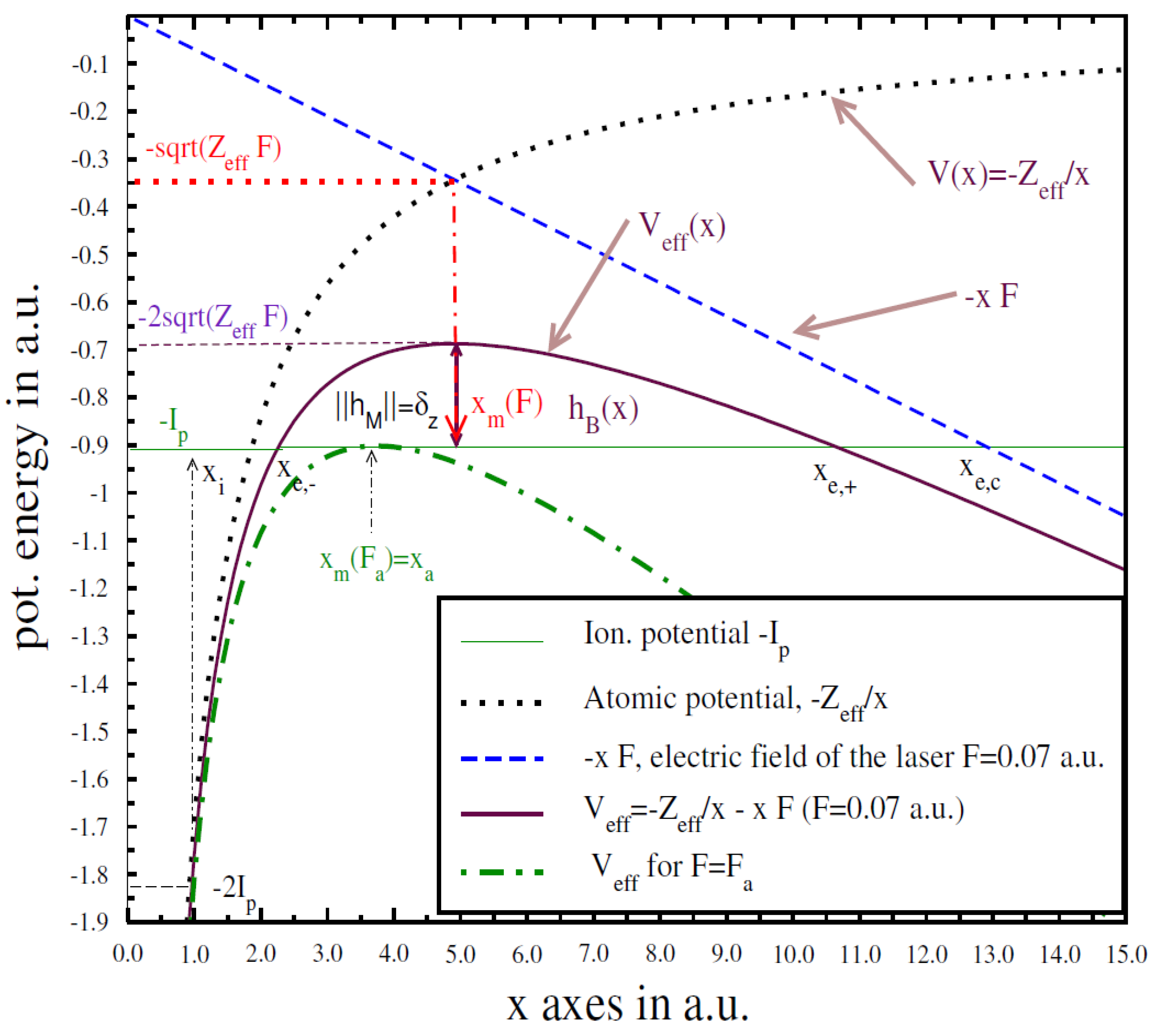
Our tunneling model was introduced in [1] (see Figure 1). We take a one-dimensional model along the x-axis as justified by Klaiber and Yakaboylu et al. [15,16]. Hereafter, we adopt the atomic units (au), where the electron’s mass and charge and the Planck constant are set to unity, . In this model, the effective potential of the atom-laser system is given by
where F (throughout this work) is the peak electric field strength (at maximum) of the laser pulse (quasistatic limit), and is the effective nuclear charge that can be found by treating the (active) electron orbital as hydrogen-like, similar to the well-known single-active-electron (SAE) model [17,18]. The choice of is easily recognized for many-electron systems and well-known in atomic, molecular, and plasma physics [19,20,21,22].
The active electron can be ionized by a short laser pulse with an electric field strength F, where ionization happens directly when F equals a threshold called atomic field strength (see below Equation (4)) [19,23], where is the ionization potential of the system (atom or molecule). However, for field strengths , ionization can happen by a tunneling mechanism, through a barrier built by the effective potential and the ionization potential, as seen in Figure 1. The barrier height at a position x is given by (see Figure 1)
that is equal to the difference between the ionization potential and effective potential of the system (atom+laser) at the position x. The crossing points of with the -line are given by [1]
is the barrier width, where is given below in Equation (5). is usually called the “classical” exit point; it is the intersection of the field line with -line, which equals what is usually called the “classical” barrier width .
We obtain the maximum from the derivative of Equation (2), . From , see Figure 1 (the lower green curve), we get the atomic field strength
Fortunately, Equation (4) can be generalized as the following. For a field strength :
the equality occurs at . Indeed, is a key quantity; it controls the tunneling process and determines the time “delay” due to the barrier () as we will see.
In Figure 1 (for details see [1]), the inner (entrance ) and outer (exit ) points, . Note that, for forward, backward tunneling, the entrance/exit, Equation (3) is exchanged, where the barrier hight (at maximum) is given by (compare Equation (4) . The energy gap is given by [2]. For (), the barrier disappears and at which the barrier-suppression ionization (BSI) starts.
In the (low-frequency) attosecond experiment, the laser field is comparable in strength to the electric field of the atom. Usually, intensities ∼10 W cm are used. It is usual to characterize the strong-field approximation (SFA) by the Keldysh parameter [24],
where is the central circular frequency of the laser pulse and denotes the Keldysh time. According to Keldysh or SFA, in Equation (6), at values , the dominant process is the multiphoton ionization (MPI). For (precisely ), the ionization (or field-ionization) happens by a tunneling process, which occurs for . SFA was developed and refined later by Faisal [25] and Reiss [26] and known under the term Keldysh–Faisal–Reiss (KFR) approximation, where the two regimes of multiphoton and tunneling are more or less not strictly defined by [27,28,29]. In the tunneling regime (for ) at a quasistatic limit, the electron does not ionize directly. It tunnels (tunnel-ionizes) though adiabatically, and escapes the barrier at the exit point to the continuum as shown in Figure 1 (a sketch for He-atom.)
With this model, we derived the following relations of the T-time [1],
As discussed in [1,2] (or ) correspond to the forward, backward tunneling, respectively. An intuitive picture is given by a physical reasoning of these relations [1] as the following: is the time delay with respect to the ionization time at atomic field strength . The latter is undoubtedly real and not zero . is the time delay for a particle to pass the barrier region and escapes at the exit point to the continuum [1]. is the time needed to reach the entrance point from the initial point , compare Figure 1. The two steps of the model coincide at the limit , and the total time becomes the ionization time at the atomic field strength , , . For , the BSI starts [30,31]. At the opposite side of the limit , and , hence, nothing happens, i.e., the electron remains in its ground state undisturbed, indicating that our model is consistent; for details, see [1,2,3]. For the first term , see below Section 3.
2. Tunneling Time and the Time Operator
2.1. Physical Reasoning
At first, we follow a reasoning in which the atomic potential plays a central role to determine the T-time. This is similar to our approach of deriving the T-time (Equation (7))) using the TEUR. The idea relies on the SFA approximation, where the electron escapes the tunnel exit with zero velocity and becomes free. It leads, in the adiabatic tunneling, to the fact that the (decreasing) atomic potential energy compensates for the dynamics directed by the electric field. Thus, in adiabatic tunneling, the momentum change (during the time interval ) due to the barrier corresponds to the change of the atomic potential, or the potential gradient in the barrier region, which we can express as the following:
In Equation (8), the factor is considered because tunneling is a half scattering (half collision) [32,33], whereas the symmetry of the process is given by forward and backward scattering [1]. Both issues will be discussed later in Section 3, where the tunneling process in SFA is viewed as a scattering process. We will also see later (Section 2.2.3) that (a time interval) in Equation (8) is the time of arrival between two points .
The constant factor is considered due to the dimensionality of the relation (note is a force field like F). Evaluating Equation (8) at the entrance/exit points as given above, leads to
In this relation, it is easy to see that for because the barrier height and width vanish, . In other words, we have to add the ionization time in the absence of the barrier, which is quantum mechanically (QMly) easily comprehensible. One tends to add T-time at atomic field strength . However, while is the ionization time at , we expect that at an enhancement in the ionization time occurs. Such an enhancement can be also inferred from the result of Aharonov et al. [9], where they discussed the TEUR and the BE-pb-GE. In our case, we have the electric field F instead of the gravitational field, and we expect the enhancement to be proportional to F relative , where the BSI region starts and the ionization becomes a classically allowed process. The enhancement can then be expressed with a simple form . Hence, the T-time as a delay time is:
which is the relation given in Equation (7). With the symmetry consideration, or changing exit, entrance points (forward, backward process), we carry out the same procedure and obtain , and hence the total time , see Equation (7). Regarding this result, the following points consider attention:
- Time like position is a relative observable [9]. One never measures its absolute values but time intervals by clocks. Throughout the present work ’s denotes time intervals, to distinguish it from a time variable usually called t.
- The way we obtained in Equation (10) is similar to the Eisenbud–Wigner–Smith (EWS) [34,35] time delay, where one adds the barrier-free motion term of the incident particle to the delay caused by the Coulomb potential of the scattering ion itself (note also the factor 1/2), where is the barrier width and v the velocity of the particle (wave packet), see further below Section 4.
- We note that our (Equation (9) fits exactly in the definition of the dwell time , the total time spent by a particle inside the barrier [34,35,36], despite the fact that the dwell time is defined in terms of transmission and reflected probabilities or coefficients, gained from the wave function of the tunneled particle(s). This makes it possible, inter alia, to link our T-time to the statistical picture of the T-time, see Section 6.
2.2. A Dynamical Time Operator
Our goal is to introduce a time operator which is a quantum mechanical (QMal) counterpart of its classical limit by the virtue of Bohr correspondence principle.
Classically and naively one usually assumes a classical dynamics with and , which leads to the Keldysh time , where according to SFA . Another classical way [2] is to take the (classical) barrier width over the (arithmetic) mean value of the velocity to escape the barrier region, , which again with leads to the Keldysh time . One notices that , which is important for the quantum counterparts, see Section 3, Section 4 and Section 5. However, it is well known that is too large and cannot describe the T-time, simply because it neglects completely the effect of the atomic Coulomb potential. Our objective is to calculate the T-time taking into account the atomic Coulomb potential. In this section, we introduce the QMal correspondence to , and, in Section 3, we encounter the correspondence to .
With the Bohr correspondence principle, we take the classical limit and make a transition to its QMal counterpart:
This is similar to the construction of the well-known Aharonow–Bohm time operator from its classical limit , see Section 3, and we assumed . The choice of the sign is related to symmetric antisymmetric form , furthermore in Section 3. The suggested notation Fujiwara–Kobe time operator (FKTO) [37,38] is explained below in Section 2.2.3. Our goal is to obtain the T-time form the time operator in Equation (11).
2.2.1. First Approach
By following Razavy [39], we use the Hamiltonian’s principle function , where , , is the Hamiltonian and are the the momentum, the coordinate, and the time variable; for details, see [39]. In our case, the Hamiltonian is not explicitly time-dependent, i.e., we take the quasistatic limit. We first show the antisymmetric form (or ), we obtain . Note that is the time of arrival discussed by Fujiwara [37] as explained in Section 2.2.3 (). Let be the Hamiltonian’s principle function and with
Accordingly, applying a time operator of the type (as in Equation (11)) with , we obtain
where as in Equation (10). A constant x − independent term C is unimportant because it cancels out for time intervals in the adiabatic tunneling dynamics. The same holds for nonadiabatic effects, which are expected to be small, especially for a short T-time period. It should be noted that nonadiabatic effects due to the oscillatory field, which causes small shifts in and a momentum drift, are small [40] and below the error bars of the experimental results [41]. p is the momentum (or momentum operator) and F the scalar electric field of the laser pulse at maximum (quasistatic limit). To get the T-time, i.e., the time to pass the barrier region, we evaluate this expression at the entrance/exit points of the tunneling region, i.e., we take the momentum difference caused by the barrier with , and, with , we get
where in the last line we applied the same argument as in Equation (10). Clearly, ionization time at atomic field strength is QMly real and not zero, and, for , a twofold time delay emerges with respect to the ionization at atomic field strength, as we noticed in Section 2.1. Actually, we can write (see Equations (10) and (14))
where can be considered as an enhancement factor, a delay caused by a field strength and the presence of the barrier . Furthermore, the first term in Equations (10) and (14) can be written in the form . Hence, we can write Equations (10) and (14) in the form
The significance of Equation (16) is obvious and its similarity to the is evident, as mentioned in the previous paragraph. Indeed, Equations (15) and (16) and the twofold delay time have a substantial consequence for the tunneling in strong field and the tunneling theory in general, a detailed investigation follows in [41] and future works. Furthermore, we see from Equations (16) and (14), due to the forward and backward tunneling , that is eliminated and the FKTO time of Equation (11) equals a pure ionization (delay) time (no tunneling part), which according to Winful (see below Equation (32)) is the self-interference part [42], , furthermore in Section 4. Finally, it is easy to show, by performing the same procedure as that of the symmetric form of Equation (11), we obtain , i.e., a constant term does not cancel out by (+) sign. However, this term is eliminated by the momentum representation as discussed by Allcock [43]; we came back to this later in Section 3.
2.2.2. Second Approach
We can obtain the same result by using what Allcock [43] called the momentum difference produced by the potential difference , in his discussion of TEUR, when he initiated the concept of time of arrival (arrival-time) in his seminal papers [43]. It actually goes back to Heisenberg original work on uncertainty relation with the Stern–Gerlach experiment [44]. Allcock defined it by
to obtain TEUR of the form
where , the distance traveled by the particle with the group velocity p, m the mass and T (actually ) is the time of transit (or equivalently arrival time) spent by the particle corresponds to the deflection angle . The momentum initiated by Allcock in Equation (17) is our dynamical observable, and we define the time operator as before in Section 2.2.1 , , where we again use a scalar field F (quasistatic limit). The difficulty is in defining . However, because L is the distance traveled by the particle (in our case the barrier region) and due to the adiabaticity, we can take on the right-hand side of Equation (17) a mean value (with ). As discussed in [45], see below Section 3, we have and we take the potential difference in the barrier region to obtain the time T corresponding to the deflection angle [43] while tunneling. For its interpretation as macroscopic quantity, see [43]. The only difference is that the deflection angle is caused by the atomic potential (scattering process), instead of the inhomogeneous field in Stern–Gerlach experiment when the atoms pass through the magnetic field. With Equation (17), we obtain
Since (the electron is decelerated), the minus sign of F is canceled, whereas for backward scattering we have , which leads to —where, unlike the Stern–Gerlach experiment, this is not the measured angle in the attoclock experiment. The delay time can be obtained with the same procedure, as we have done in Equations (10) and (14). One might argue that (the energy gap) and, by simply applying Equation (18) directly, one obtains . However, this has been discussed in [2], and it leads again to the same result . In the sense of the Allcock definition, our T-time, i.e., the time to pass the barrier region , uses the change of the atomic potential energy as a hand of the attoclock, switched on (off) at the entrance (exit) of the barrier that are themselves determined by the field strength F. However, F is quasistatic and is supposed to be known with a classical accuracy.
One notices that, in Equations (10), (14) and (19), we have calculated a time interval () from the evaluation on the two sides , of the barrier. Therefore, we get , the time interval (time difference) caused by the barrier itself (see Equation (16)), which is not the measured quantity (due to the self-interference term) in the attoclock experiment, e.g., the measurement by Eckle and Landsman et al. [4,5,6], see [1]. On the other side, constant terms cancel each other out, unless their values strongly depended on F in a nonadiabatic manner. One expects that such an effect is small, as already mentioned, since the tunneling happens in short time elapse around the peak of the field, which permits the employment of the quasistatical limit [41].
2.2.3. Final Remarks
It is worthwhile to mention that such a type of time observable or a self-adjoint operator in Equation (11) has been introduced in the past by Busch et al. [46] for a free falling particle with mass m in a gravitational (or force field) field g of the form . The operator was introduced as an example for a self-adjoint operator canonically conjugate to a Hamiltonian operator , and , where Q is the position variable (distance) and . It was our motivation to introduce the time operator in Equation (11), where in our case it is easy to show that the operator is an observable that satisfies the commutation relation with the Hamiltonian . Since the potential is a scalar quantity [47], the commutation relation is reduced to the position momentum commutation relation
We have to add that, after finishing the draft of the manuscript, we encountered earlier works [37,38] where the dynamical operator in Equation (11) and its commutation relation are discussed. Fujiwara [37] showed that a time operator of the form is well defined. This operator corresponds to the Hamiltonian and leads to time-energy uncertainty, where k is a constant uniform force field and are the position and momentum. He also showed that between two points is the arrival time. This is similar to our tunneling or delay time, compare Equation (8) (and Section 2.2.1 and Section 2.2.2). Furthermore, Kobe et al. [38] proposed the name tempus (operator) for the time operator and discussed a tempus conjugated to the Hamiltonian , where is a constant (electric) force field. Kobe et al. also showed that the Pauli argument does not apply in this case and that in general the energy and tempus satisfy the same commutation and uncertainty relations as do the operators and (the momentum and position.) The works of Fujiwara [37] and Kobe et al. [38] nicely confirm our claims of the present work. Thus, we called the time operator in Equation (11) Fujiwara–Kobe time operator .
3. Aharonov–Bohm Time Operator
In Section 2.2, we have seen that classically one obtains the Keldysh time from p/F (or Δp/F) and similarly from x/p (or ). In this section, we discuss a derivation of the T-time from the Aharonov–Bohm time operator (ABTO) the counterpart of classical form or , as we have done for the counterpart of in Section 2.2, the Fujiwara–Kobe time operator of Equation (11). The well known ABTO for a free particle with a momentum p and position x [48] is
where the second line is the momentum representation, and the third is the energy () representation, see Allcock [43], where a transformation of the wave function leads to
We first compare our T-time in Equation (7) with Equations (20) and (21). In the limit of , (ground states)
It is clear that at this limit (ground state) the electron can not escape the atom [1], whereas corresponds to the second term of ABTO in Equation (21). We will see later that correspond (forward, backward) to , the Olkhovsky time operator. Thus, the limit for reveals a connection between our T-time and ABTO. In the general case , we use Equation (21) as the following. When the electron interacts with the field, we can assume the quasistatic (adiabatic) dynamics tunneling model (QSTM). The electron moves through the barrier region adiabatically with a mean momentum , which, as discussed in [45], can be seen from
The QMal correspondence to (i.e., ) leads to as the following. With and , and noting that the QM correspondence to is , the time to reach the exit and entrance point, respectively, and their difference is the time due to the barrier itself, we get
The similarity between Equations (21) and (24) is obvious. It should be understood as a mean value due to the assumption . However, by comparing Equation (24) with Equation (20), we clearly see the difference in the minus sign. In Equations (24) and (25), the ABTO with the minus sign or corresponds to the time of arrival time (or transit time) as we have seen in Section 2.2.2, Equation (18) (where ), we discuss this later below (see Equation (29)).
Our total T-time is obtained by taking the plus sign. Then, with a mean momentum , and with Equation (20), we obtain
In fact, it has been already discussed in [1] that the symmetry of the tunneling process (forward, backward) leads respectively to and the total time , see Equation (7)—hence, the factor , which implies a relation of to the ABTO. Equation (26) might be considered as the symmetric form of ABTO, whereas Equation (24) is the antisymmetric form. QMly a symmetrization leads to a real quantity, which is obvious in Equation (26) (or (27)) and it is the time delay given in Equation (16) (see also Equation (33)). However, this is also the case in Equation (25), since is real which involves a tunnel ionization. Surprisingly, we obtain from ABTO a delay time (as given Equations (16) and (33)) of a process, in which the tunneling part (due to the barrier itself) cancels out, assigned a self-interference term by Winful [42]. The importance of this result especially to the nonadiabatic effects is discussed in [41].
Actually, as seen in Equation (27), the delay time due to the barrier itself is eliminated by the sum of the two process forward and backward in the immediate step (at second line), which invokes the question about the real, imaginary pictures of the T-time, whereas the antisymmetric form in Equation (25) eliminates the self-interference term and performs the delay time due to the barrier itself or the dwell time, compare Equation (32). A complex T-time picture can be obtained by the substitution or equivalently an imaginary barrier gap , which leads to the same result in Equation (26)
Apart from the fact that is classically allowed as discussed in [1] (see the physical reasoning of Equation (7)), which means no need to an imaginary part (i.e., is redundant), only the real part of the delay time (unlike , which is real) can be compared with the experimental and the Feynman Path Integral (FPI) results in the adiabatic tunneling picture [1,4], see discussion later in Section 6. Hence, in our view, the complex delay time of Equation (28) can not satisfactorily describe the delay time in the attoclock, Section 6.
However, the choice of the sign allows a question opened namely about the symmetric and the antisymmetric forms given by Equation (26) or Equation (24). In the former (), we obtain the self-interference term, which eliminates the tunneling part, or in other words no tunneling is involved is this case. This is in accordance with the well known observation of the numerical methods that the velocity gauge the SFA (see also Reiss [29]), in which no tunneling time is encountered, as we will discuss in Section 6. The later () corresponds to and we calculate , as done in Equations (10), (14) and (19). In this case, forward and backward processes eliminate the self-interference term and give the net time due to barrier itself, and leads to with a good agreement with the experimental result [1] in the adiabatic tunneling [1,4], as already mentioned. In terms of a classical point of view, it is nothing but the time to reach the exit point (forward tunneling ) minus the time to reach the entrance point (backward tunneling ) (multiplied by the factor for half scattering, which is of a QMal origin) and this is what makes equivalent to the time of arrival (Section 2.2.1 and Section 2.2.2), the Wigner time (further below Section 4), and the dwell time as we already noted in Section 2.1. Note, in all our time relations, that we can drop out the factor and we get, for example, , which fits exactly to the experimental data of Sainadh et al. for H-atom and the accompanied result of numerical integration of time-dependent Schrödinger equation (NITDSE). It makes, however, the agreement with the experimental data of Landsman et al. for He-atom lacking this factor.
The question is now which of the experimental data, He-atom [4], or H-atom [49] is the right choice to compare with. The factor is of a QMcal origin as we see from Equations (24) and (26); see further below Equation (29). Thus, we think that the data of Landsman et al. is reliable. On the experimental side, the difference comes from the evaluation of the experimental data, i.e., how the final photoelectron momentum distribution and the streaking offset angle difference transformed to a tunneling delay time. Finally, the same factor was also introduced by Wigner in the scattering or atomic collision to calculate the Eisenbud–Wigner time delay, as we will see in the next section. Note that it is only when is an imaginary quantity that we end with an imaginary T-time picture, the one supported by Sainadh et al. [49], see Section 4 and Section 6.
In the energy representation, the T-time is given by the form of a bilinear operator of Equation (22), see Olkhovsky [50]
where means to the left, right (or forward, backward) applied forms , . The comparison of Equations (26) and (29) with Equations (20)–(22) (and the transition ) makes it clear that ABTO can be used to derive the (or directly connected to our) T-time, though we take advantage of the QSTM. This is similar to the approach introduced by Allcock in his seminal work [43] to define the time of arrival (TOA) and obtain the TOA distribution or observable time after the classification of Busch [51] (chap. 3). In addition, it is again related to the similarity we encountered before with Fujiwara time of arrival , see Section 2.2.3. It turns out that a unified picture of the tunneling time is reliable, as we will see in Section 4.
Note that is a parameter with [52] for a small barrier when the electron escapes closer to the nucleus (large F). is better for a large barrier width when the electron moves far from the nucleus (small F), see Figure 4 of [1]. In a more reliable approximation, depends on the barrier width (or the distance to the nucleus). However, there is no such reliable approximation available so far.
4. Relation to Eisenbud–Wigner Delay Time
As we have seen in Section 3 and Equation (24), the barrier width can be used to obtain the delay time . Surprisingly, this is also useful to find a relation to Eisenbud–Wigner time or the more commonly used term mentioned in Section 2.1. The has a long history going back to atomic collision and particles scattering by a Coulombic potential. We find in [35,53] (and according to Wigner [54,55]) the following definition of the :
where are the barrier width and the velocity of the particle or the propagation velocity of the wave packet, respectively, and k is the wave vector of the monochromatic wave packet. Similar to Equation (24), we get for a tunneled electron (wave-packet) the time shift [35] due to the barrier ()
where again ( as mentioned above) is the mean velocity of the particle (propagation velocity of the wave-packet) in the tunneling region. Obviously, one has to add the barrier-free term to get the total EWS-time [35]. Thus, adding the self-interference term (see Equation (32)) or (Equation (16)) as we have done in Equations (10), (14), (19) and (26), we get immediately the time delay . Clearly, corresponds to the . Although this result is unexpected, we think it is not surprising. Then, from Equation (30), we see immediately the similarity to Equations (22) and (29) in the energy form , where the phase is related to the semiclassical action. We note that such a unified T-time picture was already found by Winful [42] for the quantum tunneling of a wave packet or a flux of particles scattering on a potential barrier. Winful showed in his work that the group delay or the Wigner time delay can be written in the form
where is the dwell time which corresponds to our as mentioned in Section 2, and is a self-interference term which corresponds to our in Equations (16) and (33), see further below Section 6. Recently, Han et al. [56] tried also to find a unified T-time picture, but they claimed that the concept of T-time depends on the model used to derive it. We think that the unified picture brought by Winful is more reliable, especially since it fits well with our result.
It is worthwhile to note that Bray et al. used a similar point of view with a semiclassical Keldysh–Rutherford (RK) model based on the Rutherford scattering [33,57]. They found a Coulombic origin of the attoclock offset angle (ACOA). Nevertheless, they claimed to confirm an imaginary T-time picture, which was justified by NITDSE with a short-range potential, see Section 6.
In the imaginary time picture as also done by Bray et al., one claims that experimentally measured ACOA is rooted to the tail of the potential, whereas the T-time is imaginary and its real part is zero (instantaneous tunneling) with a decomposition of the form (), where are the saddle point solution, the exit time and the T-time, respectively, see [49,58]. According to [58], the exit time is the time at which the electron leaves the tunneling barrier, or the ionization time that is in the tunneling picture corresponds to the moment at which the electron emerges in the classically allowed region [58].
As we found in this section, permits a scattering mechanism interpretation for the T-time where the ACOA corresponds to a real because and hence are real quantities.
An important point is that we now clearly see that the factor in Equation (30) (and the same in ) enters because the tunneling is half scattering. Taking a second factor by symmetrization (anti-symmetrization) as done in Equations (24)–(27) (and (28)) corresponds to forward, backward scattering. In our view, this again shows that the result of Landsman et al. [4] for He-atom [1], is more reliable than the result of Sainadh et [49] for H-atom [7] (which lacks a factor ), as already mentioned in Section 3.
Therefore, the adiabatic tunneling process can also be understood in term of scattering in which the ACOA is due to the scattering by Coulombic potential in the barrier region (not the tail of the potential) and corresponds to the T-time with real quantities (i.e., a real T-time), whereas Bray et al. [33,57] as mentioned above claims that their RK model confirms the imaginary time picture or that the ACOA is due to the tail of the Coulombic potential by comparing the model to a numerical result. In [57] by a comparison to experimental results for H-atom [49], they found that the latter confirms the dependence of RK-scattering curve (where I is the intensity of the laser pulse), which is in accordance with an dependence of the T-time, e.g., Equation (15) with an additional nonlinear term , which is quite smaller than unity (the first term).
Thus far, we see that our real T-time picture is highly consistent and fundamental. However, we have to add in regard to imaginary tunneling picture that it is common (rather fundamental) in QM that two pictures exist for a QMal physical process or phenomena [7]. Indeed, the debate continues and a complete picture of the T-time is not reached so far.
5. Discussion
In Section 2.2, we introduced a time operator and calculated the T-time Equations (14) and (19). Our approach is supported by the works of Busch et al. [46], Fujiwara [37], and Kobe et al. [38]. We also have shown in Section 3 that the Aharonov–Bohm time operator leads to the same result Equation (24), by taking advantage of a QSTM or an adiabatic tunneling with a mean value of the momentum . A similar conclusion is found in Section 4 with the Eisenbud–Wigner delay time . It turns out that the specific form of the time operator is not crucial, and a dynamical variable such p of the system under consideration maintains the time observable through an operator form, which represents this time observable. This is similar to the classical case or limits , which lead to the Keldysh time , as mentioned in Section 3. Thus, time operators representing a dynamical variable (intrinsic time) are equivalent.
Furthermore, to our knowledge, this is the first time where one encounters a close relation between T-time delay and time of arrival, see Section 2.2 last paragraph and Section 3. Time of arrival is widely used to calculate T-time. However, the usual belief is that time delay and time of arrival are two different definitions of the time observable, i.e., they result in two time intervals (different ’s) for the same process in quantum systems. According to our present work, we argue that intrinsic time can be represented equivalently by different well defined (dynamical) operators. The most known types, among others, are the delay time and the time of arrival. It is worthwhile to explain what we mean with the above stated well defined. An example is the definition of the Mandelstam–Tamm time operator (MTTO) [59,60,61] ( are two operators of the system, and is the wave function)
Recently, Gray et al. [60] argued that the TEUR-version of MTTO depends on the states that are not eigenvectors of an observable. It means that the Mandlestam–Tamm time (MT-time) is the infimum of the ratio of static uncertainty to dynamic uncertainty per unit time (see discussion in [2]). Messiah [62] used MTTO to define “the characteristic time of evolution”, whereas Gray et al. claimed that this formulation recommends itself since it does not promise too much. They also provided what they called a (mathematical) precise definition of MTTO [60]. However, following Kullie [2], the MTTO can be, in fact, brought in line with the time of arrival of ABTO and the time delay in Equation (7), by using p as a dynamical observable. Furthermore, this contrasts the claim of Orlando et al. [63] that the MT-time is equal to the Keldysh time. Our conclusion is that, under the same conditions, well-defined time operators by a dynamical observable equivalently represent one and the same intrinsic (dynamical) time or time observable of the system (called tempus by Kobe et al. [38]), a clock dynamically attached to the system. The remaining question concerns the equivalence between different time operators, which are defined on the basis of different dynamical observables of the system. In the present work, solely p was used as a dynamical observable.
6. Attoclock and Tunneling Time in Strong Field Interaction
Attosecond angular streaking experiments (termed attoclock) have triggered a hot debate about T-time, whether it is a real or an imaginary quantity. In adiabatic tunneling, for example [4,5,6] with a Helium (He) atom, we have found that T-time is real. It is a delay time with respect to the ionization at atomic field strength [1,2,3]. In an experiment with H-atoms, Sainadh et al. [49] argued using a short-range potential model and NITDSE that tunneling is instantaneous. Hence, they support the point of view that T-time, i.e., the time to traverse the barrier region, is an imaginary quantity. In [7], we found that the measured data in the experiment with H-atom of Sainadh et al. and the accompanied NITDSE [8,49] fits very well to our real T-time picture (Equation (7)). Solely the factor of (1/2) is still unclear; it is absent in the experimental data of Sainadh et al. [8,49], unlike the data of Landsman et al. [4] for the He atom, as discussed in Section 3 and Section 4. Furthermore, according to the imaginary time picture, one also claims that time is a parameter in QM and not an observable. Hence, no time operator exists in QM in line with the well known Pauli theorem. However, the later point has been clarified and the list of references is too large to be specified; see, for example, [11,12,13,37,38,39,45,64,65,66,67] and the references therein. The present work is a step in this direction.
Despite this, Rost et al. [68] argued that, thanks to the attoclock experiments with He- and H-atoms, one can be sure that a reasonably defined T-time is zero in these cases. Furthermore, Rost et al. concluded that, using classical back propagation of an ionized wave packet (determined QMly by Schrödiger equation), one arrives at the conclusion that the T-time defined at the exit point (as defined in their work) is zero for single-electron dynamics, see Ni et al. [69]. Tunneling is a QMal manifestation and a classical point of view is not appropriate anyway, a deterministic T-time is not expected. Furthermore, although they found a positive time at the exit point by back propagating with the position-based criterion, they claimed that the T-time is zero and the criterion can be considered as a misinterpretation of the attoclock experimental data based on models that do not take full and consistent account for nonadiabaticity, with the argument that they found a high non-tunneled fraction [70], we come back later to this important point. In the same work [69], they found that a static energy-based (again in their notation) adiabatic tunneling criterion fails completely.
The core point in the result (Equation (7)) of our tunneling model is the real T-time to overcome the barrier region as a delay time with respect to the ionization time at atomic field strength; the latter is undoubtedly real and QMly does not vanish. The issue becomes more evident by rewriting Equation (15) in the form (see also Equation (16))
where both terms are time delays and real, the second term is real because is a real quantity for [1]. The relation to , , and of ABTO that we have discussed in Section 3 and Section 4 confirms our point of view, in particular that provides a similar picture of a scattering particle on a Coulombic potential. However, it is not yet entirely clear whether the origin of the delay time is the Coulombic barrier, due to the similarity with , or due to the tail of the Coulomb potential, as claimed by th imaginary T-time picture [49,58]. The latter enforces a , which is not reflected in our comparison of the experimental data, especially for F values near the atomic field strength , where shows a good agreement with the experimental result [1]. Our model uses the length gauge or the dipole approximation of the interaction Hamiltonian [2] due to the Göppert–Mayer gauge-transformation [71]. However, to claim that it is a kind of a position criterion seems vague, apart from the fact that Equation (15) fits well with the experimental results, as shown in [1]. We think that the work of Ni et al. [69] indicates that numerical methods, such as back propagation including NITDSE imply a dependence on the applied concepts, e.g., the back propagation with the different criteria in the work of Ni et al. [69]. Hence, they end with inconclusive results and interpretations. A drawback of their approach is that they only consider backward propagation, which is not sufficient to give a clear tunneling picture (forward propagation is not considered).
Actually, we have already encountered such a matter in the work of Orlando et al. [63], where they claimed to obtain Keldysh time as a lower limit of the T-time from the NITDSE and the MTTO. However, we found in [2] and discussed in the present work that applying the MTTO in our tunneling model leads to the T-time relation in Equation (7), which agrees well with the experimental results. Reiss [29] divided the strong field approximation methods into two categories, strong electric-field approximation (SEFA) and strong propagating-field approximation (SPFA). He argued that they are critically different. The SEFA employs a tunneling model that trends to an adiabatic limit at low frequencies; the SPFA does not invoke the tunneling concept. This could be one of the reasons why Ni et al. get different results by applying different criteria. It is worth noting that earlier works using NITDSE [72,73] have also reached a similar conclusions like Ni et al. As a consequence, the conclusion of Ni et al. of an imaginary T-time, though possible, is not a closing answer and does not tell much concerning the T-time and tunneling theory in general. The imaginary T-time picture is in line with the fact that the tunneling is classically forbidden. This is important; nevertheless, it is not instructive in the case it obscures an insight and otherwise accessible conceptual understanding (See Carver Mead, the Nature Of Light What Are Photons, www.cns.caltech.edu). It offers a picture of tunneling mechanisms among other pictures, a situation that is common in QM. A complete picture to the tunneling in strong field science is still not available, where certainly it is crucial to distinguish between adiabatic and nonadiabatic tunneling.
Our T-time concept for adiabatic tunneling opens a new insight for the understanding and of a fundamental importance to the tunneling theory in general, as mentioned in Section 1. Note that a complex time point of view, i.e., real and imaginary parts, such as the one brought by Torlina et al. [58], would not change our conclusion. The difference is that Torlina et al. [58] claim that the measurement of the attoclock, the real part, corresponds to the tail of the atomic Coulomb potential by using a short-range potential model, whereas in our picture the atomic potential energy at the exit point of a single-active electron model determines the uncertainty in the energy and, by the virtue of TEUR, we get the real delay time measured in the attoclock; see our detailed discussion in [3]. The utilization of TEUR in our model is important to compare with the statistical point of view of the T-time and to the tunneling theory in general, as we will see in the following.
The measurement data in both experiments with He- and H-atom are of a statistical nature. Landsman et al. have shown [4] a good agreement between the experimental result and the FPI. Demir et al. [74] came to the same result of the T-time using a statistical approach to the T-time (SATT) based on FPI. Camus et al. [75] claim that the agreement between theory and experiment in their work with Ar-, Kr-atom provides clear evidence for a nonzero T-time delay, however without clear details about their tunneling picture, i.e., adiabatic or nonadiabatic, which is certainly a crucial point. In our T-time model, we have found a good agreement with FPI of Landsman et al. for He-atoms [1], and with NITDSER of Sainadh et al. for H-atoms [7]. Thus, as far as adiabatic tunneling is considered, we think the question is rather how to compare our result and model with the FPI, NITDSE and other statistical and wave packet dynamics model calculations. We will now discuss a possibility to resolve this puzzle.
First, as known, a single electron model and statistical or probabilistic interpretation inherently coexist in the QM. One thinks about a single electron atom such as the H-atom, the Bohr model, the radial Schrödiger equation, and the Born interpretation of its wave function.
Second, our model is not alone or a pure semiclassical single-active electron model because our T-time is derived by the virtue of the TEUR [1], and, in this sense, it is a QMal model with a direct relation to the statistical or probabilistic point of view, see Landsman et al. [4,35]. It is not the time spent by a single electron moving over or through a barrier having an energy less than the barrier height, which is a classical inadequate picture to offer an understanding to our result and the T-time in general. Having such a classical picture in mind does not help to find the correct answer or the right interpretation to the T-time.
In his work, Galapon [76] constructed a time of arrival operator for a square potential barrier and calculated its expectation value for a wave packet. By a comparison to the result of Eckle et al. [5,6] for He-atoms, he showed that only the above-the-barrier components of the momentum distribution of the incident wave packet contribute to the traversal time to cross the barrier region. In statistical methods or wave packet dynamics, one considers the momentum distribution which corresponds to a collective incident of a stream of particles (a statistical ensemble) upon a potential barrier. From this point of view, what Galapon found is that the particles partially tunnel in real time (traversal time). Thus, in terms of FPI [35], this is the part that corresponds to the amount of the transmitted particles or transmission amplitude. It is the part of the wave function that corresponds to a specific time that the electron spends inside the potential barrier [35]. In this sense, one can imagine that our T-time would correspond, in terms of a transmission amplitude, to the time of the part of the wave function that tunneled (transmitted) the potential barrier. For example, at a field strength , the ionization rate is the part of ionized atoms (transmission amplitude of the wave function) relative to the amplitude of the total wave function of the system, which corresponds to the total number of the atoms. In this respect, in our model, we quantify tunneling through the energy gap (potential barrier) and T-time using TEUR, which is equivalent to quantifying it through the transmission amplitude of the wave function. This follows in particular from the good agreement of our T-time with FPI [4,35] and SATT [74] for He-atoms. We see now why Ni et al. [69] have found a high non-tunneled fraction as mentioned above (using a position criterion). The tunneling probability is always less than unity and only at reaches unity, see Delone [77] (p. 72). They ignore the fact that tunneling unlike ionization depends on the probability amplitude or transmission and reflection amplitudes and coefficients. The tunneled fraction corresponds to the part of the transmission amplitude, which corresponds to the T-time and , which agree with the experimental result in the adiabatic tunneling [1,4,35].
At the atomic field strength , the T-time is the ionization time (compare Equations (15) and (33)), at which the ionization rate equals unity [77] (p. 72), where the barrier disappears and the BSI region starts, which is a classically allowed process. Actually, we can express our views with a simple form in terms of relative probability amplitude, . Hence, we find that is an enhancement factor similar to Equation (15). One notices that is the QMal limit and for any time measurement through an interaction with a field [9], see [1,2].
In a way, our approach is tied to the Heisenberg picture of the QM, where the dynamics are performed by the operators acting on the time-independent state vectors, which are represented by a basis in the phase space. The expectation values are then extracted information by virtue of the operators acting on the sates vectors, where the probability character of the expectation value corresponds to the probability amplitude or the factor . However, certainly the calculation of is a difficult task, whereas our approach offers a simple procedure to calculate the tunneling time by exploiting the TEUR [1].
Therefore, we think that our tunneling model is in line with the statistical, probabilistic point of view, e.g., such as FPI, the wave packet dynamics and wave function methods or NITDSE. It might explain the good agreement of our T-time [1] with FPI of Landsman et al. [4], and NITDSE of Sainadh et al. [8,49] (apart from the factor as already discussed). This point of view is supported by the similarity between the delay time (interval) due to the barrier itself and the dwell time , see Section 2.1. The latter is defined statically by the transmission and reflection coefficient or amplitudes of the wave function [35] (in our picture forward, backward scattering). In addition, similarly, it is supported by the agreement with the unified tunneling picture of Winful (Equation (32)), see Section 4. This way we showed that our real T-time conciliates with various interpretations and pictures, it is in this sense sturdy, thorough, and fundamental.
Finally, one might argue that the imaginary T-time picture is physically more reliable, see Rost et al. [68], but why then is the ACOA caused by the tail of the potential [49,58] if the energy gap is mainly covered by the nonadiabatic effects? There are several concerns with this picture. 1. It ignores the self-interference term, Equations (32) and (33), which also exists for a zero-range potential. 2. We have already seen from in Equation (30) that the ACOA is likely caused by a scattering mechanism due to the Coulomb potential and not solely due to the tail of the potential. 3. It ignores that the time to reach the entrance point (Equation (7), see Figure 1), is a classically allowed process. Furthermore, the electron becomes a free particle at the exit point, when it gains the energy through the nonadiabaticity. It is then less affected by the tail of the Coulombic potential, which is screened by the field [45]. Otherwise, we do have to rely on the adiabatic tunneling picture, where our real T-time model, together with the statistical or probabilistic time interpretation as discussed above, offers a reasonable picture in which the nonadiabatic effects are small and not crucial to the ACOA or the T-time. Where the nonadiabaticity due to the oscillatory field is smaller than the error bars, as already mentioned, and, in our opinion, it is reflected by the spread of the points in the experimental result, compare the figures given in [4]. Further discussion is given in [41], and we follow this issue in future works.
7. Conclusions
In this work we showed that our T-time can be obtained from a time operator. It is a delay time with respect to an ionization time at the atomic field strength; hence, it is an intrinsic dynamical time and is similar to different dynamical time definitions such as time of arrival, classified as an observable time by Busch [78]. Different types of time operators are discussed, where the conclusion is that, under the same conditions, dynamical time operators equivalently represent the intrinsic (dynamical) time observable of the system, termed as the tempus of the (evolving) system by Kobe et al. [38]. In this sense, the well known definitions, delay time, and time of arrival represent the same dynamical time observable of the system under consideration. A similar unified picture is found by Winful as discussed in Section 4. From the similarity with the EWS-time and dwell time , it should be noted that time intervals of the tempus of the system are or should be identical, despite resulting from different definitions. We found that the symmetric (antisymmetric) ABTO (likewise FKTO) is related to our total time (), where the forward and backward tunneling eliminate the delay time due to the barrier itself (the self-interaction term), respectively. We follow this issue in future works where adiabatic and nonadiabatic tunneling will be considered. Additionally, we discussed the attoclock and the real versus imaginary T-time picture and concluded with the remark that our tunneling model, which is based on the single-active electron approximation and the TEUR, is in line with the statistical or probabilistic picture of the T-time defined by the probability amplitudes of tunneling ionization such as FPI and SATT.
Funding
This research received no external funding.
Acknowledgments
I would like to thank Martin Garcia from Theoretical Physics of the Institute of Physics at the University of Kassel for his kind support. I am indebted to an anonymous reviewer for fruitful remarks.
Conflicts of Interest
The author declares no conflict of interest.
References
- Kullie, O. Tunneling time in attosecond experiments and the time-energy uncertainty relation. Phys. Rev. A 2015, 92, 052118. [Google Scholar] [CrossRef] [Green Version]
- Kullie, O. Tunneling time in attosecond experiments, intrinsic-type of time. Keldysh, and Mandelstam–Tamm time. J. Phys. B At. Mol. Opt. Phys. 2016, 49, 095601. [Google Scholar] [CrossRef]
- Kullie, O. How to understand the tunneling in attosecond experiment? Bohr-Einstein photon box Gedanken experiment, tunneling time and the wave particle duality. Ann. Phys. 2018, 389, 333. [Google Scholar] [CrossRef] [Green Version]
- Landsman, A.S.; Weger, M.; Maurer, J.; Boge, R.; Ludwig, A.; Heuser, S.; Cirelli, C.; Gallmann, L.; Keller, U. Tunneling Time in Ultrafast Science is Real and Probabilistic. Optica 2014, 1, 343. [Google Scholar] [CrossRef] [Green Version]
- Eckle, P.; Pfeiffer, A.N.; Cirelli, C.; Staudte, A.; Dörner, R.; Muller, H.G.; Büttiker, M.; Keller, U. Attosecond Ionization and Tunneling Delay Time Measurements in Helium. Science 2008, 322, 1525. [Google Scholar] [CrossRef] [PubMed]
- Eckle, P.; Smolarski, M.; Schlup, F.; Biegert, J.; Staudte, A.; Schöffler, M.; Muller, H.G.; Dörner, R.; Keller, U. Attosecond angular streaking. Nat. Phys. 2008, 4, 565. [Google Scholar] [CrossRef] [Green Version]
- Kullie, O. Tunneling time in attosecond experiment for hydrogen atom. J. Phys. Commun. 2018, 2, 065001. [Google Scholar] [CrossRef]
- Sainadh, U.S.; Xu, H.; Wang, X.; Atia-Tul-Noor, A.; Wallace, W.C.; Douguet, N.; Bray, A.; Ivanov, I.; Bartschat, K.; Kheifets, A.; et al. Attosecond angular streaking and tunnelling time in atomic hydrogen. arXiv 2017, arXiv:1707.05445. [Google Scholar] [CrossRef] [Green Version]
- Aharonov, Y.; Reznik, B. “Weighing” a Closed System and the Time-Energy Uncertainty Principle. Phys. Rev. Lett. 2000, 84, 1368. [Google Scholar] [CrossRef] [Green Version]
- Auletta, G.; Fortunato, M.; Parisi, G. Quantum Mechanics; Cambridge University Press: Cambridge, UK, 2009. [Google Scholar]
- Galapon, E.A. Paulis theorem and quantum canonical pairs: The consistency of a bounded self-adjoint time operator canonically conjugate to a hamiltonian with non-empty point spectrum. Proc. R. Soc. Lond. A 2002, 458, 451. [Google Scholar] [CrossRef] [Green Version]
- Galapon, E.A. Self-adjoint time operator is the rule for discrete semi-bounded hamiltonians. Proc. R. Soc. Lond. A 2002, 458, 2671. [Google Scholar] [CrossRef] [Green Version]
- Galapon, E.A. What could have we been missing while Pauli’s theorem was in force? arXiv 2002, arXiv:quant-ph/0303106. [Google Scholar]
- Garrison, J.; Wong, J. Canonically conjugate pairs, uncertainty relations, and phase operators. J. Math. Phys. 1970, 11, 2242. [Google Scholar] [CrossRef]
- Klaiber, M.; Yakaboylu, E.; Bauke, H.; Hatsagortsyan, K.Z.; Keitel, C.H. Under-the-Barrier Dynamics in Laser-Induced Relativistic Tunneling. Phys. Rev. Lett. 2013, 110, 153004. [Google Scholar] [CrossRef]
- Yakaboylu, E.; Klaiber, M.; Bauke, H.; Hatsagortsyan, K.Z.; Keitel, C.H. Relativistic features and time delay of laser-induced tunnel ionization. Phys. Rev. A 2013, 88, 063421. [Google Scholar] [CrossRef] [Green Version]
- Muller, H.G. Numerical simulation of high-order above-threshold-ionization enhancement in argon. Phys. Rev. A 1999, 60, 1341. [Google Scholar] [CrossRef]
- Tong, X.M.; Lin, C. Foundation of the modern physics. J. Phys. B 2005, 38, 2593. [Google Scholar] [CrossRef]
- Augst, S.; Meyerhofer, D.D.; Strickland, D.; Chin, S.L. Laser Ionization of noble gases by Coulomb-barrier suppression. J. Opt. Soc. Am. B 1991, 8, 858. [Google Scholar] [CrossRef]
- Schlüter, D. Gaunt Factors for Free-Free Transitions in the Fields of the First, Ions of the Rare Gases, Calculated in the Scaled Thomas-Fermi Approximatione. Z. Phys. D 1987, 6, 249. [Google Scholar] [CrossRef]
- Lange, R.; Schlüter, D. Free-free emission continuum of weakly non-ideal argon plasmas. J. Quant. Spectrosc. Radiat. Transf. 1992, 48, 153. [Google Scholar] [CrossRef]
- Dreissigacker, I.; Lein, M. Quantitative theory for the lateral momentum distribution after strong-field ionization. Chem. Phys. 2013, 414, 69. [Google Scholar] [CrossRef]
- Augst, S.; Strickland, D.; Meyerhofer, D.D.; Chin, S.L.; Eberly, J.H. Tunneling Ionization of Noble Gases in a High-Intensity Laser Field. Phys. Rev. Lett. 1989, 63, 2212. [Google Scholar] [CrossRef] [PubMed]
- Keldysh, L.V. Ionization in the field of a strong electromagnetic wave. Zh. eksp. teor. Fiz. 1964, 47, 1945, [English translation: Soviet Phys. JETP 1965, 20, 1307]. [Google Scholar]
- Faisal, F.H.M. Multiple absorption of laser photons by atoms. J. Phys. B 1973, 6, L89. [Google Scholar] [CrossRef]
- Reiss, H.R. Effect of an intense electromagnetic field on a weakly bound system. Phys. Rev. A 1980, 22, 1786. [Google Scholar] [CrossRef]
- Reiss, H.R. Energetic electrons in strong-field ionization. Phys. Rev. A 1996, 54. [Google Scholar] [CrossRef]
- Reiss, H.R. Unsuitability of the Keldysh parameter for laser fields. Phys. Rev. A 2010, 82, 023418. [Google Scholar] [CrossRef]
- Reiss, H.R. The Strong-Field Approximation without the tunneling concept. arXiv 2019, arXiv:1810.12106v4. [Google Scholar]
- Delone, N.B.; Kraǐnov, V.P. Tunneling and barrier-suppression ionization of atoms and ions in a laser radiation field. Phys.-Uspekhi 1998, 41, 469. [Google Scholar] [CrossRef]
- Kiyan, I.Y.; Kraǐnov, V.P. Above-barrier ionization of the hydrogen atom in a superstrong optical field. Sov. Phys. JETP 1991, 74, 429. [Google Scholar]
- Torlina, L.; Ivanov, I.A.; Walters, Z.B.; Smirnova, O. Time-dependent analytical R-matrix approach for strong-field dynamics. II. Many-electron systems. Phys. Rev. A 2012, 86, 0430409. [Google Scholar]
- Bray, A.W.; Eckart, S.; Kheifets, A.S. Keldysh-Rutherford Model for the Attoclock. Phys. Rev. Lett. 2018, 121, 123201. [Google Scholar] [CrossRef] [PubMed] [Green Version]
- Hauge, E.H.; Støvneng, J.A. Tunneling times: A critical review. Rev. Mod. Phys. 1989, 61, 917. [Google Scholar] [CrossRef]
- Landsman, A.S.; Keller, U. Attosecond science and the tunneling time problems. Phys. Rep. 2015, 547, 1. [Google Scholar] [CrossRef]
- Smith, F.T. Lifetime Matrix in Collision Theory. Phys. Rev. 1960, 118, 349. [Google Scholar] [CrossRef]
- Fujiwara, I. Rational Construction and Physical Signification of the Quantal Time Operator. Prog. Theor. Phys. 1980, 64, 18–27. [Google Scholar] [CrossRef] [Green Version]
- Kobe, D.H.; Aguilera-Navarro, V.C. Derivation of the energy-time uncertainty relation. Phys. Rev. A 1994, 50, 933–938. [Google Scholar] [CrossRef] [Green Version]
- Razavy, M. Quantum-mechanical conjugate of the hamiltonian operator. Il Nuovo Cim. B (1965-1970) 1969, 63, 271. [Google Scholar] [CrossRef]
- Hofmann, C.; Zimmermann, T.; Zielinski, A.; Landsman, A.S. Non-adiabatic imprints on the electron wave packet in strong field ionization with circular polarization. New J. Phys. 2016, 18, 043011. [Google Scholar] [CrossRef]
- Kullie, O. Tunneling/Ionization time in the nonadiabatic attoclock, Multiphoton process versus tunneling in strong field interaction. Work in preparation.
- Winful, H.G. Delay Time and the Hartman Effect in Quantum Tunneling. Phys. Rev. Lett. 2003, 91, 260401. [Google Scholar] [CrossRef] [PubMed] [Green Version]
- Allcock, G.R. The Time of Arrival in Quantum Mechanics, I. Formal Considerations. Ann. Phys. 1969, 53, 253–285. [Google Scholar] [CrossRef]
- Heisenberg, W. Über den anschaulichen Inhalt der quantentheoretischen Kinematik und Mechanik. Z. Phys. 1927, 43, 172. [Google Scholar] [CrossRef]
- Kullie, O. Tunneling Time in Attosecond Experiments and Time Operator in Quantum Mechanics. Mathematics 2018, 6, 192. [Google Scholar] [CrossRef] [Green Version]
- Busch, P.; Grabowski, M.; Lahti, P.J. Time observables in quantum theory. Phys. Lett. A 1994, 191, 357. [Google Scholar] [CrossRef]
- Bauer, M. Tunneling in attosecond optical ionization and a dynamical time operator. Phys. Rev. A 2017, 96, 022139. [Google Scholar] [CrossRef] [Green Version]
- Aharonov, Y.; Bohm, D. Time in the Quantum Theory and the Uncertainty Relation for Time and Energy. Phys. Rev. 1961, 122, 1649. [Google Scholar] [CrossRef]
- Sainadh, U.S.; Xu, H.; Wang, X.; Atia-Tul-Noor, A.; Wallace, W.C.; Douguet, N.; Bray, A.; Ivanov, I.; Bartschat, K.; Kheifets, A.; et al. Attosecond angular streaking and tunnelling time in atomic hydrogen. Nature 2019, 568, 75. [Google Scholar] [CrossRef] [Green Version]
- Olkhovsky, V.S. Time as a Quantum Observable, Canonically Conjugated to Energy, and Foundations of Self-Consistent Time Analysis of Quantum Processes. Adv. Math. Phys. 2009, 1, 859710. [Google Scholar] [CrossRef]
- Muga, G.; Mayato, R.S.; Egusquiza, I. (Eds.) Time in Quantum Mechanics, Lecture Notes in Physics 734; Springer: Berlin/Heidelberg, Germany, 2008; Volume 1. [Google Scholar]
- Clementi, E.; Raimondi, D.L. Atomic Screening Constants from SCF Functions. J. Chem. Phys. 1963, 38, 2686. [Google Scholar] [CrossRef]
- De Carvalho, C.A.A.; Nussenzveig, H.M. Time dely. Phys. Rep. 2002, 364, 83. [Google Scholar] [CrossRef]
- Wigner, E.P. Lower Limit for the Energy Derivative of the Scattering Phase Shift. Phys. Rev. 1955, 98, 145. [Google Scholar] [CrossRef]
- Eisenbud, L.E. The Formal Properties of Nuclear Collisions. Ph.D. Thesis, Princeton University, Princeton, NJ, USA, 1948. unpublised. [Google Scholar]
- Han, M.; Ge, P.; Fang, Y.; Yu, X.; Guo, Z.; Deng, X.M.Y.; Gong, Q.; Liu, Y. Unifying Tunneling Pictures of Strong-Field Ionization with an Improved Attoclock. Phys. Rev. Lett. 2019, 123, 073201. [Google Scholar] [CrossRef] [PubMed]
- Serov, V.V.; Bray, A.W.; Kheifets, A.S. Numerical attoclock on atomic and molecular hydrogen. Phys. Rev. A 2019, 99, 063428. [Google Scholar] [CrossRef] [Green Version]
- Torlina, L.; Morales, F.; Kaushal, J.; Ivanov, I.; Kheifets, A.; Zielinski, A.; Scrinzi, A.; Muller, H.G.; Sukiasyan, S.; Ivanov, M.; et al. Interpreting Attoclock Measurements of Tunnelling Times. Nat. Phys. 2015, 11, 503. [Google Scholar] [CrossRef] [Green Version]
- Mandelstam, L.; Tamm, I. The Uncertainty Relation Between Energy and Time in Non-relativistic Quantum Mechanics. J. Phys. USSR 1945, 9, 249. [Google Scholar]
- Gray, J.E.; Vogt, A. Mathematical analysis of the Mandelstam–Tamm time-energy uncertainty principle. J. Math. Phys. 2005, 46, 052108. [Google Scholar] [CrossRef]
- Sukhanov, A.D. Generalized energy-time uncertainty relation. Theor. Math. Phys. 2000, 125, 1489. [Google Scholar] [CrossRef]
- Messiah, A. Quantum Mechanics; North-Holland: Amsterdam, The Netherlands, 1961; Volume 1. [Google Scholar]
- Orlando, G.; McDonald, C.R.; Protik, N.H.; Vampa, G.; Brabec, T. Tunneling time, what does it mean? J. Phys. B 2014, 47, 204002. [Google Scholar] [CrossRef]
- Fock, V.; Krylov, N. On the uncertainty relation between time and energy. J. Phys. USSR 1947, 11, 112. [Google Scholar]
- Han, D.; Noz, M.E.; Kim, Y.S.; Son, D. c-number time energy uncertainty relation in the quark model. Phys. Rev. D 1983, 27, 3032. [Google Scholar] [CrossRef]
- Busch, P. On the Energy-Time Uncertainty Relation. Part I: Dynamical Time and Time Indeterminacy. Found. Phys. 1990, 20, 1. [Google Scholar] [CrossRef]
- Busch, P. On the Energy-Time Uncertainty Relation. Part II: Dynamical Time and Time Indeterminacy. Found. Phys. 1990, 20, 33. [Google Scholar] [CrossRef]
- Michael Rost, J.; Saalmann, U. Attoclock and tunnelling time. Nat. Photonic 2019, 13, 439. [Google Scholar] [CrossRef]
- Ni, H.; Saalmann, U.; Rost, J.M. Tunneling exit characteristics from classical backpropagation of an ionized electron wave packet. Phys. Rev. A 2018, 97, 013426. [Google Scholar] [CrossRef]
- Ni, H.; Saalmann, U.; Rost, J.M. Tunneling criteria and a nonadiabatic term for strong-field ionization. Phys. Rev. A 2018, 98, 013411. [Google Scholar] [CrossRef]
- Göppert-Mayer, M. Über Elementarakte mit zwei Quantensprüngen. Ann. Phys. 1931, 401, 273. [Google Scholar] [CrossRef]
- Bauer, D.; Milošević, D.B.; Becker, W. Strong-field approximation for intense-laser-atom processes: The choice of gauge. Phys. Rev. A 2005, 72, 023415. [Google Scholar] [CrossRef] [Green Version]
- Bauer, J. Slow-frequency–high-intensity limit of the Keldysh-Faisal-Reiss theory. Phys. Rev. A 2006, 73, 023421. [Google Scholar] [CrossRef]
- Demir, D.A.; Güner, T. Statistical approach to tunneling time in attosecond experiments. Ann. Phys. 2017, 386, 291. [Google Scholar] [CrossRef] [Green Version]
- Camus, N.; Yakaboylu, E.; Fechner, L.; Klaiber, M.; Laux, M.; Mi, Y.; Hatsagortsyan, K.Z.; Pfeifer, T.; Keitel, C.H.; Moshammer, R. Experimental Evidence for Quantum Tunneling Time. Phys. Rev. Lett. 2017, 119, 023201. [Google Scholar] [CrossRef] [PubMed]
- Galapon, E.A. Only Above Barrier Energy Components Contribute to Barrier Traversal Time. Phys. Rev. Lett. 2012, 108, 170402. [Google Scholar] [CrossRef] [PubMed]
- Delone, N.B.; Kraǐnov, V.P. Multiphoton Processes in Atoms, 2nd ed.; Springer: Berlin/Heidelberg, Germany, 2000. [Google Scholar]
- Busch, P. Time in Quantum Mechanics; Muga, J.G., Mayato, R.S., Egusquiza, I.L., Eds.; Lecture Notes in Physics; Springer: Berlin/Heidelberg, Germany, 2008; Volume 734, pp. 73–105. [Google Scholar]
Figure 1.
(Color online) Graphic display of the potential and the effective potential curves, the two inner and outer points , the barrier width . , is the ionization potential, is the effective nuclear charge, and F is the electric field strength of the laser pulse at maximum. the “classical exit” point and the position at the maximum of the barrier height . , is the atomic field strength, see text. The plot is for He-atom in the single-active-approximation model with and . Note for systems with different the overall picture stays the same.

© 2020 by the author. Licensee MDPI, Basel, Switzerland. This article is an open access article distributed under the terms and conditions of the Creative Commons Attribution (CC BY) license (http://creativecommons.org/licenses/by/4.0/).
Share and Cite
MDPI and ACS Style
Kullie, O. Time Operator, Real Tunneling Time in Strong Field Interaction and the Attoclock. Quantum Rep. 2020, 2, 233-252. https://0-doi-org.brum.beds.ac.uk/10.3390/quantum2020015
AMA Style
Kullie O. Time Operator, Real Tunneling Time in Strong Field Interaction and the Attoclock. Quantum Reports. 2020; 2(2):233-252. https://0-doi-org.brum.beds.ac.uk/10.3390/quantum2020015
Chicago/Turabian StyleKullie, Ossama. 2020. "Time Operator, Real Tunneling Time in Strong Field Interaction and the Attoclock" Quantum Reports 2, no. 2: 233-252. https://0-doi-org.brum.beds.ac.uk/10.3390/quantum2020015