Nonlocal Interferences Induced by the Phase of the Wavefunction for a Particle in a Cavity with Moving Boundaries

1
Institute for Quantum Studies, Chapman University, Orange, CA 92866, USA
2
Laboratoire de Physique Théorique et Modélisation, CNRS Unité 8089, CY Cergy Paris Université, 95302 Cergy-Pontoise CEDEX, France
*
Author to whom correspondence should be addressed.
Quantum Rep. 2020, 2(4), 514-528; https://0-doi-org.brum.beds.ac.uk/10.3390/quantum2040036
Submission received: 12 October 2020
/
Revised: 26 October 2020
/
Accepted: 27 October 2020
/
Published: 30 October 2020
Abstract
:We investigate the dynamics of a particle in a confined periodic system—a time-dependent oscillator confined by infinitely high and moving walls—and focus on the evolution of the phase of the wavefunction. It is shown that, for some specific initial states in this potential, the phase of the wavefunction throughout the cavity depends on the walls motion. We further elaborate a thought experiment based on interferences devised to detect this form of single-particle nonlocality from a relative phase. We point out that, within the non-relativistic formalism based on the Schrödinger equation (SE), detecting this form of nonlocality can give rise to signaling. We believe this effect is an artifact, but the standard relativistic corrections to the SE do not appear to fix it. Specific illustrations are given, with analytical results in the adiabatic approximation, and numerical computations to show that contributions from high-energy states (corresponding to superluminal velocities) are negligible.
1. Introduction
While quantum nonlocality based on multi-particle entanglement is well-recognized, single particle nonlocality remains controversial. The primary candidate of the latter would be the Aharonov–Bohm effect [1]. In the Aharonov–Bohm (AB) effect, the wavefunction phase evolution is deemed to be nonlocal. The phase contains dynamical and geometric components. Both the dynamical [2,3] and the geometric [4] components are ascribed a nonlocal origin. Nevertheless, the nonlocal character of the Aharonov–Bohm effect has been disputed on the ground that electromagnetic forces might be able to account for the AB phase [5,6]. The nonlocal character of the quantum phase therefore remains controversial (note that the non-local aspects due to the dynamics of a single particle wavefunction should not be conflated with single particle entanglement between modes and spatially separated wavepackets, see e.g., [7] for an overview of the latter).
In this work, we investigate the same issue of phase nonlocality of a single quantum particle but we focus on an entirely different system. The system we deal with is a time-dependent linear oscillator confined by infinitely high walls, one of which is moving. Put differently, our system is an infinite well subjected to a time-dependent harmonic potential and in which one of the well’s walls has an oscillatory motion. The first reason for choosing this system is that analytic solutions of the time-dependent Schrödinger equation are known [8]. The second, less mundane, reason is that such systems, and in particular their simplest variant (a box with a linearly moving wall), have long been suspected of manifesting some form of nonlocality [9,10,11,12,13].
It was indeed conjectured [9,10] that the moving wall could nonlocally change the phase of a wavepacket at the center of the box that remained localized far from the wall. While this conjecture proved to be incorrect [14], it was recently noted [12] that, when a quantum state had a non-zero probability amplitude near the wall, a linearly expanding wall induced instantaneously a current density at any point of the box. We note for completeness that systems with moving boundaries are of current interest in practical schemes in the field of quantum engines or in atomic spectroscopy [15,16,17].
In the present paper, we are interested in the phase evolution of a quantum state in a confined oscillator with a moving wall. More precisely, we focus on a particle in a cavity whose left wall is fixed (say at ) but whose right wall oscillates, while inside the cavity the particle is subjected to an oscillator potential. We require the initial state to be spread throughout the cavity, but the phase is only measured near the static wall (at ) of the cavity. For an appropriately chosen initial state and Hamiltonian parameters, the time evolved state after one period of oscillation is simply , where is a global phase. The same initial state evolving in an identical cavity but with a different motion for the moving wall does not yield the same global phase, although the cause of the different phase evolution is due to a potential that is different only in a small region near the moving wall.
Naturally, these phases are not observable, but we elaborate a thought experiment that allows an observer located near the fixed wall to nonlocally infer the phase at time by splitting the state into a spatial superposition at and observing the resulting interference after the parts are recombined. Since the non-relativistic Schrödinger equation does not impose an upper bound for energies or velocities, the observer near the fixed wall can even infer the phase before a light signal has the time to propagate from the moving wall. This feature could give rise to some form of signaling (although our observer needs to accumulate ensemble statistics in order to deduce the phase difference and cannot infer anything in a single shot). We should stress that we do not believe this signaling is physical, but rather that it is an artifact of employing a non-relativistic formalism. However, we show that it is not clear how the tiny contributions from high-energy eigenstates (with superluminal velocities) can account for the observed change in the global phase.
We start by introducing the Hamiltonian of the system and the solutions to the Schrödinger equation (Section 2). We then focus on the phase evolution in particular by comparing the cases in which the Hamiltonian is identical except at the moving boundary (Section 3). In the latter case, we give the solution in the adiabatic approximation. Section 4 deals first with the nonlocal nature of the quantum phase, and then explains how the formalism can result in signaling. A specific protocol is given. We then illustrate our results by choosing a specific potential and boundary motion (Section 5).
2. Time-Dependent Oscillators with Moving Walls
2.1. Time-Dependent Linear Oscillators
A quantum time-dependent linear oscillator is a system comprising a particle of mass m subjected to the Hamiltonian,
where we assume in this work to be T-periodic, . The solutions of the Schrödinger equation,
depend on an initial condition and on appropriate boundary conditions, e.g., . These solutions can be obtained in semi-analytical form. Several methods have been developed, from the one relying on obtaining the eigenfunctions of dynamical invariants (see [18] and references therein), pioneered by Lewis and Riesenfeld [19], to more general Lie system-based approaches [20].
A time-dependent linear oscillator can be confined in a box bounded by infinitely high fixed walls (FW). Let denote the width of the well, ie the distance between the two walls. The corresponding Hamiltonian is given by,
and the solutions of the Schrödinger equation must respect the boundary conditions . There are no general methods to solve the confined time-dependent (or the confined standard harmonic) oscillator (see [21,22] and references therein for specific cases).
2.2. Confined Oscillator with Time-Dependent Boundary Conditions
We now confine the time-dependent oscillator in a box with a moving outer wall, i.e., the box has length with boundaries at and , as shown in Figure 1. The Hamiltonian is similar to Equations (3) and (4):
This system is mathematically intricate as it involves a different Hilbert space at each time t and standard quantities such as the the time derivative are ill-defined. A proper approach [23,24] involves using time-dependent unitary transformations mapping the time-dependent boundary conditions to fixed ones. Only then can the general methods based on the Floquet theorem be employed (see [25] for the derivation of the Floquet operator for a box with an arbitrary periodic motion of the wall). Fortunately, for specific boundary conditions and related frequencies , explicit solutions of the Schrödinger equation are known [8]. It can indeed by verified by direct substitution that,
obeys the Schrödinger equation,
with the boundary conditions,
provided that,
The are not instantaneous eigenstates but form a set of orthogonal basis functions that can be used to determine the evolution of an arbitrary initial state. We choose in this work and therefore to be periodic functions. An important property is the phase increment after a full period. Indeed, comparing and leads immediately to,
with,
Hence, after a full cycle, a time-dependent oscillator with moving walls in state returns to its initial state except for a phase increment . Following Aharonov and Anandan [26], the total phase can be parsed into a “dynamical” part encapsulating the usual phase increment due to the instantaneous expectation value of the Hamiltonian and a “geometric” part . The dynamical phase,
is readily computed [14] and the nonadiabatic geometric phase, is then obtained as,
Note that, in the case of a free confined Hamiltonian, it is possible to obtain a general expression for the geometric phase associated to a cyclic adiabatic evolution in terms of the chosen boundary conditions [27].
3. The Wavefunction Phase Evolution
3.1. Phase and Walls Motions
The phase [Equation (12)] is a property of the entire wavefunction, although part of the phase increment is due to the walls’ motion. To see this, we compare two oscillators that have exactly the same potential everywhere except in the vicinity of the outer wall. To this end, we examine three different cases:
- (I)
- an oscillator with the outer wall moving according to some function and with a time-dependent frequency obeying Equation (10),
- (II)
- an oscillator with the outer wall moving according to a function and with a time-dependent frequency also obeying Equation (10), and
- (III)
- an oscillator with the outer wall moving according to the function but evolving in the potential of the first case, .
Note that the solutions in Case I are given by Equation (7) with the cavity length , and the solutions in Case II are given by Equation (7) with . However, Case III is a mixture: the time-dependent frequency is given by Equation (10) with while the boundary condition is , and therefore the solutions are not of the form (7).
We take to be very close to and with the same period T. The idea is to compare the phase in Cases I and III, which evolve in the same potential except in the region near the walls, since the boundary conditions, depending, respectively, on and , are slightly different. We start from the same initial state of the type given by Equation(7). To have the same initial state, we must impose and Picking functions for which leads to an initial state,
with .
The total phase increment after one period and is given by Equation (12). Case III, however, does not respect Equation (10) and therefore does not fit in the framework developed in Section 2.2. We look for a perturbative solution in this case. Note that in Case III there is no reason to expect the existence of a global phase increment, although, due to the continuity of the wavefunction, we can expect that, if and are close enough, the phase increment after one full cycle will not deviate far from a constant value in the vicinity of a given point. We are interested in the phase in the vicinity of , which is the farthest region from the moving walls.
3.2. Phase Increment in Case III
3.2.1. Quantum State Evolution
Let denote the solution of the Schrödinger equation for the Case III mentioned in the preceding subsection. Let denote the basis functions of Equation (7) with Since obeys the boundary condition , we look for a solution in the form,
with the initial condition being,
Applying the Schrödinger equation with for to the right hand-side of Equation (16) and recalling that leads to,
and by projecting we obtain,
The integral can be readily computed, yielding,
for , the integral becomes,
In the adiabatic case, only the coefficient of the initial state is non-zero, . There is no summation in Equation (19) and is obtained by solving analytically the differential equation (see Equation (26)). The integral in that equation may be obtained analytically for specific choices of and ; otherwise a simple numerical integration is in order.
In the generic (nonadiabatic) case, there are no analytical solutions. We obtain numerical solutions by writing first Equation (18) as
and then multiplying this equation by and integrating. The basis functions are orthogonal, and the remaining non-trivial integrals
can be integrated analytically without difficulty. This leaves us with a system of linear first-order (in time) coupled equations for , subject to the initial condition This formally infinite system is truncated by setting an upper bound in the sum of Equation (22). The choice of depends on the desired accuracy of the solutions: since as k increases, it should be checked that throughout the x and t intervals over which the solutions are computed (z is the numerical zero).
Note that the dynamical phase for Case III can be obtained by computing,
3.2.2. Adiabatic Approximation
To obtain the coefficients in closed form, approximations need to be made. The simplest regime is the “adiabatic” approximation which involves neglecting the contribution of basis states other then the initial one, as specified by the initial condition (17). Hence, and is obtained from Equation (19) by keeping only the diagonal contribution, yielding,
Note that the adiabatic approximation employed here is similar but not strictly equivalent to the standard adiabatic theorem (see, e.g., Ch. 2 of [28]), since the adiabatic theorem deals with instantaneous eigenstates of a single Hamiltonian, whereas here we are employing basis functions of the Case II Hamiltonian in the Schrödinger equation with the Case III Hamiltonian. Plugging this back into Equation (16), we see that within our approximation the total phase after one full cycle is,
The first term is the Case II phase , and the second term appears as a correction. Part of this correction is due to the dynamical phase, which is different from Case II since the potential in Case III is the one from Case I, leading to the dynamical phase given in Equation (25). The remaining part of this correction, proportional to , is a geometric term due to the boundary conditions.
The adiabatic approximation is expected to hold when and are almost identical. Then, to discriminate the phase of the different cases mentioned above, it is crucial that and differ significantly. Indeed, appears as a correction to [Equation (27)], so that ensuring that while still having typically implies high values of n and/or small values of m [see Equation (12)].
3.2.3. Generic Case
In general, the adiabatic approximation will of course not be valid. The generic case is characterized by a set of non-negligible coefficients with k lying in the interval ,. Indeed, initially only is non-vanishing, and the coupling between and the different coefficients falls off as for large k (see Equations (19) and (20)). Since here we are interested in short time evolutions, we can expect that only a few basis states centered on contribute to the expansion in Equation (16). While there is no simple analytical formula giving the phase increment in this generic situation, it is straightforward to compute numerically the wavefunction in Case III and from there extract the phase increment after one full cycle. Note that in general there is no reason to expect that, similarly to Equation (11), the wavefunction after one period is equal to the initial wavefunction up to a global phase. We can however expect, for reasonable choices of and the phase to be slowly varying (as a function of x) and approximately constant in the neighborhood of , which is our region of interest in the protocols described below.
4. Nonlocality and Signaling
4.1. Nonlocal Origin of the Quantum Phase
Let us go back to the three cases described in Section 3.1, from the point of view of an observer placed in the neighborhood of . Let the system be initially prepared in a state given by Equation (7). Since we want to be independent of whether the system evolves with boundary function or , we must enforce and for simplicity we set . Let us assume the observer, say Alice, can determine the phase difference between the initially prepared state and the state after one period . Alice can therefore discriminate Case I from Case II, since the phases at and [Equation (12)] are different. However, the Hamiltonian is also different in these two cases, a point Alice could have checked by making local measurements in her vicinity, so she will not be surprised by finding different phases depending on whether the system evolved in Case I or Case II.
However, when comparing Cases I and III, the Hamiltonian is identical except in the vicinity of the wall’s position: only the wall’s motion differs in Cases I and III. Nevertheless, the total phase at is different, including in the region where Alice is standing. Hence, the phase difference between Cases I and III must be attributed to the potential in the region near the opposite wall. Since the wall can be arbitrarily far from the region, we can say that the phase difference appears to be due to local potentials varying in an arbitrarily remote region: the phase increment, as it appears in the region near the static wall at , has a nonlocal origin.
4.2. Signaling
Let us still assume that Alice has access to the phase difference between the wavefunctions at and (such a protocol is given immediately below), and further assume that the walls are sufficiently far away so that the time it takes for a light signal emitted from the moving (right) wall to reach her position near the fixed left wall, , is larger than the period T of the wall’s motion. By measuring the phase difference, she can determine whether the wall is moving according to or Alice can thus discriminate Case I from Case III before a signal sent from the moving wall, say by Bob, reaches her. In principle, by choosing different functions , Bob could send signals to Alice superluminally.
4.3. Protocol
We describe here one possible protocol that formally leads to signaling. Indeed, by changing the motion of the wall at , Bob is able to change the global phase evolution, which is an instantaneous and measurable effect that occurs everywhere in the cavity. Because of this, Bob can send a message by choosing how the wall moves after , and then Alice can detect this choice by making local measurements near . To make sure the message is clearly resolved, Alice and Bob need to share a large ensemble of identical cavities, and Bob must make the same choice of motion for all of them. Provided that Alice completes her measurements well before , this message is sent faster than c.
In order for Alice to perform her measurement, the cavity needs to have a bit more structure (see Figure 2). Suppose that, in the y-direction, the cavity has the potential of a fixed infinite square well of width , with one wall at , the other at , and a beam splitter at , which runs the full length from to . The harmonic potential is initially turned off and the walls are stationary.
The initial state of the particle is , where is the cavity state we have been discussing, and is a Gaussian wave-packet with average y-velocity which begins well-localized at , as displayed in Figure 2. We assume that this experiment finishes quickly enough that the spreading of this wave-packet can be ignored.
When the particle strikes the beam splitter, half of the wavefunction is reflected and half is transmitted. At the moment the packets have passed the beam splitter, the harmonic potential is turned on throughout the cavity, and the wall segment at and begins to move according to . Bob also chooses at this moment whether the wall segment at and begins to move according to (Message 0) or (Message 1). The two half-packets propagate along y then bounce off their respective walls, and meet back at the beam splitter, a period after they left it—which is incidentally when again. The harmonic potential and wall motion are then turned off once more.
The cavity is tuned so that, if Bob chose , then, when the two half-pulses meet, they interfere destructively for and constructively for , and thus the particle always ends up in the region . However, if Bob chose , then the two half-pulses would have accumulated a phase difference of before they meet again, and the interference would no longer be perfectly constructive/destructive.
At , Alice places detector at and detector at . Each detector spans and the entire effective width of the Gaussian packet in the y-direction. If Bob chose the wall motion , only can fire since the particle is in the upper half of the cavity, but since the detectors have a small width relative to the cavity length L, the probability that Alice detects a particle in each cavity is only approximately . Hence, Alice and Bob need to share a large ensemble of identical cavities as this allows Alice to count the total number of clicks on the detectors and . In particular, if Bob has chosen , the phase generated by the wall motion leads to destructive interference in the lower part of the cavity, so Alice can only obtain clicks on , and thus , indicating Message 0 (where is the average number of detector clicks per cavity); instead, if Bob’s wall moves as , then this generates a phase difference that leads to a phase difference in both cavities, and thus , indicating Message 1 (an example derivation of can be found in Section 5). As a result, provided and assuming that counting the clicks takes a negligible time, Alice is able to receive Bob’s message before a signal traveling at c could reach her.
The faster-than-light communication protocol can be summarized as follows:
- A large ensemble of quantum particles (e.g., electrons) are identically prepared at in identical cavities, as shown in Figure 2.
- At , Bob chooses to send Message 0 by setting the motion of his wall in every cavity of the ensemble to or Message 1 by setting their motion to .
- At , Alice places detector at and detector at in every cavity of the ensemble. The ratio indicates Message 0 and indicates Message 1.
5. Illustration
5.1. System Hamiltonian
For the purpose of illustration, let us choose the following wall motion functions,
where and . Both walls move according to Equation (28), but with the different amplitudes, . Index is Case I from Section 3.1, with , and is Case III, with the same and an independent . The Hamiltonian for Cases I and III is obtained from Equations (5), (6) and (28) as,
that is the potential differs only in the interval between and .
In Case I, the phase increment is calculated from Equation (12) as,
In Case III, the phase increment can be obtained in the adiabatic approximation from Equation (27), giving explicitly,
The adiabatic approximation requires here , with , and ,.
5.2. Examples Displaying Nonlocality
We now give a couple of numerical examples based on the Hamiltonians (29) and (30) with parameters giving rise to nonlocality. As stated above, this is defined when the period, now is smaller than the time it takes a light signal to travel from the initial moving wall’s position to the static leftward wall, The numerical computations for the Case III wavefunctions are carried out by solving the truncated version of the coupled system defined by Equations (18) and (19). This is similar to numerical methods used in previous related works [12,29] except that the expansion basis is taken to be the solutions of Case II rather than the instantaneous eigenstates (i.e., those obeying ).
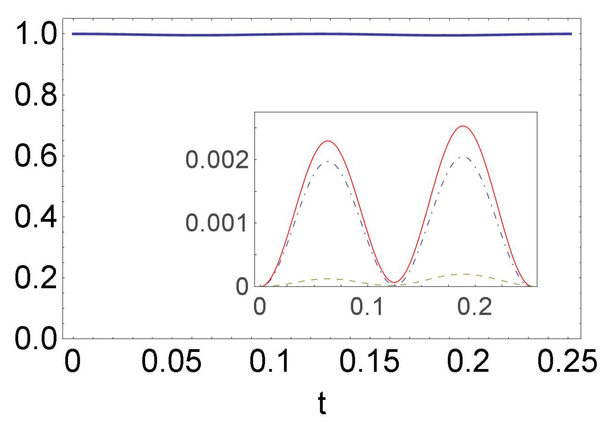
For both examples, we take the initial state to be the ground state (see Equation (17) with ). The first illustration concerns an instance for which the adiabatic approximation holds. This can be verified by solving numerically for the coefficients . The coefficients with the largest amplitude , and are plotted in Figure 3. It can be seen that, for the initial state, remains almost always equal to unity for all times , while is small and is negligible (for the other coefficients , with , is even smaller).
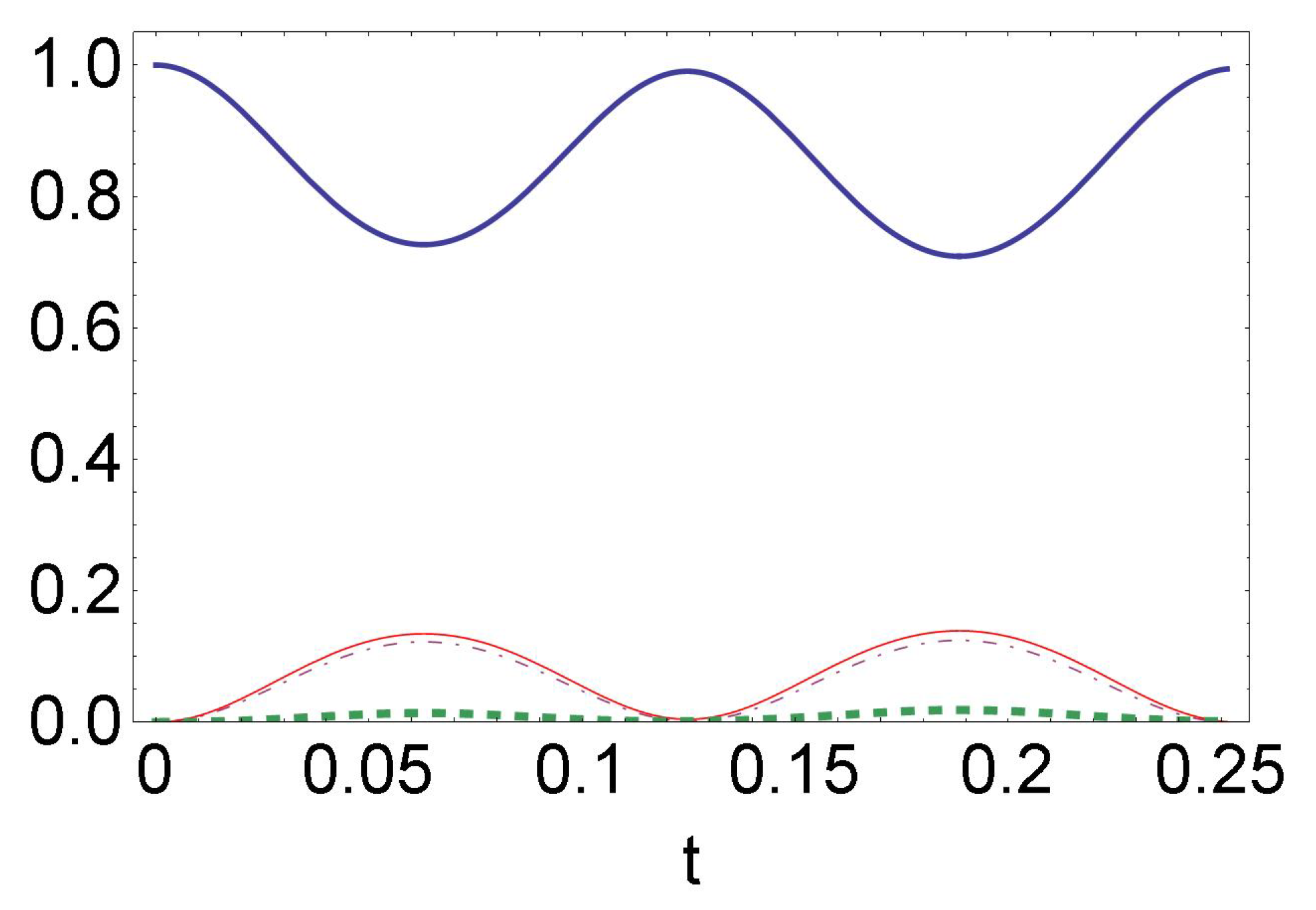
In the second illustration, we keep the same parameters as for the first illustration except for the amplitude of the oscillating boundary, , which is significantly increased. While is still the dominant term, and are not negligible, as seen from the numerical results shown in Figure 4.
The phase difference at between the Case III and Case I cavities is shown in Figure 5. Recall that, in Case III, Equation (11) is not exactly verified—it holds approximately when (and in particular when the adiabatic approximation holds) but varies with x as becomes significantly different from . For our present purposes, the important feature is that varies slowly with x in the spatial region in which the phase difference will be measured (i.e., in the vicinity of . This is the case in the illustrations shown here.
A crucial feature for our argument on nonlocality concerns the absence of superluminal velocities. As mentioned above, the Schrödinger equation does not impose any bounds on energy eigenstates and admits solutions of arbitrarily high energies, hence involving superluminal velocities. We therefore need to check that no such states are needed in order to account for the effect we observe in our illustrations. From a numerical standpoint, it is straightforward to compute the average velocity and its standard deviation as a function of time and check it lies below the light velocity. As a rule of thumb, each function of Equation (7) has a velocity component obtained by decomposing the standing wave into the forward and backward traveling waves. The average velocity of, e.g., the forward traveling wave , is obtained as,
Alternatively, and can be obtained straightforwardly for the standing wave . In both cases, when time-averaged over a period, this gives a velocity of the order of , where is the average cavity length over a period. We therefore need to ensure only modes for which contribute, a condition apparently fulfilled by large masses and long cavities. On the other hand, to obtain a non-negligible phase difference between Cases I and III, we need n to be large, and m and to be small (see Section 3.2).
We have seen that in the adiabatic case working with the sole function is sufficient to account for the phase difference . In the example given in Figure 3, we have and . In the nonadiabatic example, more basis states need to be included; rather than setting a cut-off value in the sum (16) as a function of the value of , we use a stricter criterion requiring that the numerically computed phase displays variations negligible compared to and becomes constant as additional basis states are included in the expansion. This is illustrated in Figure 6, where it is seen that states up to must be included in the expansion (16); this state corresponds to a velocity (note however that, for the overall state the time averages over a period for and are much lower, respectively, and ). Note that the nonadiabatic regime is characterized by the fact that the non-diagonal terms in Equation (19) contribute. As shown in Section 3.2, these non-diagonal terms are expected to increase for large values of L and when the time-dependent frequencies and become significantly different. Therefore, to avoid the contribution of high energy modes (leading to superluminal velocities), we need rather large cavity lengths, and hence we see that the nonadiabatic regime is generic and the adiabatic case an exception. In our numerical example, however, we have chosen a low value of L and only changed the value of the oscillating wall frequencies (through the values of the parameter ) in order to illustrate the adiabatic and nonadiabatic cases employing the same cavity except for the oscillation amplitude.
6. Discussion
We investigate a system in which different boundary conditions induce different cyclic global phases on the total wavefunction, although the system evolves in identical potentials except near the boundary. This global phase is acquired by the entire wavefunction, although part of the phase generation takes place at the boundary. In this sense, it appears to be a nonlocal effect. To observe a nonlocal signal, we perform an interference experiment wherein this effect produces a nonlocal relative phase instead of a global phase.
We assume this appears possible only because of some artifact of non-relativistic quantum mechanics; it is indeed well-known that the Schrödinger equation admits eigenstates of arbitrarily high energies, implying arbitrarily high velocities. In a recent work [12], a similar type of nonlocality in a related system (a cavity in free space expanding linearly in time) was seen on the current density. Signaling could be obtained by making weak measurements of the momentum. Discarding the contribution of high energy basis states (that would propagate superluminally) was somewhat subtle: several hundred basis states needed to be included in order to compute the current density, and, while a basis restricted to subluminal states achieved the nonlocal effect, convergence of the current density demanded the inclusion of a more complete basis, containing superluminal states.
Here, instead, nonlocality arises through a periodic evolution of the phase. Weak measurements are not required to observe signaling. Very few basis states are involved in the computation, and, in the adiabatic limit, only a single state contributes. Nevertheless, although it looks unlikely that high energy superluminal states are responsible for the form of nonlocality we investigate here, it remains impossible to totally discard their role. Indeed, from a formal standpoint, a complete basis in a non-relativistic setting will necessarily include superluminally propagating states. The adiabatic limit is of course an approximation.
A second question that comes up concerns possible specific features in the system employed. Indeed, the present system combines two features, each of which is known to lead to difficulties. First, the confining potential is modeled as an infinite wall, whereas inside the cavity the potential is a time-dependent oscillator. Introducing infinite discontinuities is known to lead to peculiar dynamical features [30,31]. It should be noted however that, in the static cases (the standard particle in a box problem or a harmonic oscillator confined by static walls [32]), these peculiarities are not known to lead to any unphysical results. Second, dealing with time-dependent boundary conditions involves formally [14,23] a different Hilbert space at each time t. The time-dependent unitary mapping to a standard problem—a problem with fixed boundary conditions defined in a single Hilbert space—yields a Hamiltonian with a time-dependent mass, so that the (local) boundary conditions are mapped to a (delocalized) time-dependent parameter. We remark that mapping the time-dependence of parameters in the original system to their parameters in the transformed system is a generic mathematical property of time-dependent unitary transformations, and this mapping has in general no bearing on the physical properties of the original system.
Conversely, one may wonder whether the nonlocal effect mentioned here could be generic, in the sense that the wavefunction phase has a global character even if it includes dynamical effects due to a potential that is non-vanishing only in a small region over which the wavefunction is defined. This would be analogous to the nonlocal features of the Aharonov–Bohm phase [1,3,4]. However, the AB effect is significantly different from the features characterizing the present problem: it is an electromagnetic effect, the vector potential is non-vanishing over the entire region in which the wavefunction is defined, the individual phases are gauge-dependent, and there is no signaling [33,34].
To conclude, we investigate the evolution of the phase of the wavefunction of a particle trapped in a confined time-dependent oscillator with a moving boundary and find the phase to be nonlocal. We also show that a protocol based on phase interference detection can give rise to signaling, an apparent nonphysical artifact. Further work is needed to pinpoint the different sources accounting for this behavior within the formalism and to see if it is possible to discriminate the effects due to dynamical nonlocality from the artifacts leading to signaling.
Author Contributions
M.W. and A.M. both authors conceived the idea, prepared the draft, wrote and reviewed the manuscript. All authors have read and agreed to the published version of the manuscript.
Funding
This research received no external funding.
Acknowledgments
This research was supported (in part) by the Fetzer Franklin Fund of the John E. Fetzer Memorial Trust.
Conflicts of Interest
The authors declare no conflict of interest.
References
- Aharonov, Y.; Cohen, E.; Rohrlich, D. Nonlocality of the Aharonov-Bohm effect. Phys. Rev. A 2016, 93, 042110. [Google Scholar] [CrossRef] [Green Version]
- Aharonov, Y. Non Local Phenomena and the Aharonov-Bohm Effect. In Proceedings of the International Symposium Foundations of Quantum Mechanics, Tokyo, Japan, 16–24 August 1983; Nakajima, S., Murayama, Y., Tonomura, A., Eds.; Foundations of Quantum Mechanics in the Light of New Technology. World Scientific: Singapore, 1997; pp. 10–19. [Google Scholar]
- Popescu, S. Dynamical quantum non-locality. Nat. Phys. 2010, 6, 151. [Google Scholar] [CrossRef]
- Anandan, J. Non local aspects of quantum phases. Ann. L’IHP A 1988, 49, 271. [Google Scholar]
- Vaidman, L. Role of potentials in the Aharonov-Bohm effect. Phys. Rev. A 2012, 86, 040101(R). [Google Scholar] [CrossRef] [Green Version]
- Batelaan, H.; Becker, M. Dispersionless forces and the Aharonov-Bohm effect. EPL 2015, 112, 40006. [Google Scholar] [CrossRef] [Green Version]
- Terra Cunha, M.O.; Dunningham, J.A.; Vedral, V. Entanglement in single-particle systems. Proc. R. Soc. A 2007, 463, 227. [Google Scholar]
- Makowski, A.J.; Dembinski, S.T. Exactly solvable models with time-dependent boundary conditions. Phys. Lett. A 1991, 154, 217. [Google Scholar] [CrossRef]
- Greenberger, D.M. A new non-local effect in quantum mechanics. Physica B 1988, 151, 374. [Google Scholar] [CrossRef]
- Makowski, A.J.; Peplowski, P. On the behaviour of quantum systems with time-dependent boundary conditions. Phys. Lett. A 1992, 163, 143. [Google Scholar] [CrossRef]
- Wang, Z.S.; Wu, C.; Feng, X.-L.; Kwek, L.C.; Lai, C.H.; Oh, C.H.; Vedral, V. Geometric phase induced by quantum nonlocality. Phys. Lett. A 2008, 372, 775–778. [Google Scholar] [CrossRef]
- Matzkin, A.; Mousavi, S.V.; Waegell, M. Nonlocality and local causality in the Schrödinger equation with time-dependent boundary conditions. Phys. Lett. A 2018, 382, 3347. [Google Scholar] [CrossRef] [Green Version]
- Colin, S.; Matzkin, A. Non-locality and time-dependent boundary conditions: A Klein-Gordon perspective. EPL 2020, 130, 50003. [Google Scholar] [CrossRef]
- Matzkin, A. Single particle nonlocality, geometric phases and time-dependent boundary conditions. J. Phys. A 2018, 51, 095303. [Google Scholar] [CrossRef] [Green Version]
- Elouard, C.; Jordan, A.N. Efficient Quantum Measurement Engines. Phys. Rev. Lett. 2018, 120, 260601. [Google Scholar] [CrossRef] [Green Version]
- Duffin, C.; Dijkstra, A.G. Controlling a Quantum System via its Boundary Conditions. Eur. Phys. J. D 2019, 73, 221. [Google Scholar] [CrossRef]
- Wang, D. Photodetachment of the H—ion in a quantum well with one expanding wall. Phys. Rev. A 2018, 98, 053419. [Google Scholar] [CrossRef]
- Lopes de Lima, A.; Rosas, A.; Pedrosa, I.A. On the quantum motion of a generalized time-dependent forced harmonic oscillator. Ann. Phys. 2008, 323, 2253. [Google Scholar] [CrossRef]
- Lewis, H.R.; Riesenfeld, W.B. An Exact Quantum Theory of the Time-Dependent Harmonic Oscillator and of a Charged Particle in a Time-Dependent Electromagnetic Field. J. Math. Phys. 1969, 10, 1458. [Google Scholar] [CrossRef]
- Cariñena, J.F.; de Lucas, J. Lie systems: Theory, generalisations, and applications. Dissertationes Mathematicae 2011, 479, 1. [Google Scholar] [CrossRef] [Green Version]
- Razavy, M. Time-dependent harmonic oscillator confined in a box. Phys. Rev. A 1991, 44, 2384. [Google Scholar] [CrossRef]
- Ghosh, P.; Ghosh, S.; Bera, N. Classical and revival time periods of confined harmonic oscillator. Indian J. Phys. 2015, 89, 157. [Google Scholar] [CrossRef]
- Mostafazadeh, A. Perturbative calculation of the adiabatic geometric phase and particle in a well with moving walls. J. Phys. A 1999, 32, 8325. [Google Scholar] [CrossRef]
- Di Martino, S.; Facchi, P. Quantum systems with time-dependent boundaries. Int. J. Geom. Methods Mod. Phys. 2015 12, 1560003. [CrossRef] [Green Version]
- Seba, P. Quantum chaos in the Fermi-accelerator model. Phys. Rev. A 1990, 41, 2306. [Google Scholar] [CrossRef]
- Aharonov, Y.; Anandan, J. Phase change during a cyclic quantum evolution. Phys. Rev. Lett. 1997, 58, 1593. [Google Scholar] [CrossRef]
- Facchi, P.; Garnero, G.; Marmo, G.; Samuel, J. Moving walls and geometric phases. Ann. Phys. 2016, 372, 201. [Google Scholar] [CrossRef] [Green Version]
- Bohm, A.; Mostafazadeh, A.; Koizumi, H.; Niu, Q.; Zwanziger, J. The Geometric Phase in Quantum Systems; Springer: Berlin, Germany, 2003. [Google Scholar]
- Glasser, M.L.; Mateo, J.; Negro, J.; Nieto, L.M. Quantum infinite square well with an oscillating wall. Chaos Solitons Fract. 2009, 41, 2067. [Google Scholar] [CrossRef]
- Aslangul, C. Surprises in the suddenly-expanded infinite well. J. Phys. A 2008, 41, 075301. [Google Scholar] [CrossRef]
- Belloni, M.; Robinett, R.W. The infinite well and Dirac delta function potentials as pedagogical, mathematical and physical models in quantum mechanics. Phys. Rep. 2014, 540, 25. [Google Scholar] [CrossRef]
- Gueorguiev, V.G.; Rau, A.R.P.; Draayer, J.P. Confined one-dimensional harmonic oscillator as a two-mode system. Am. J. Phys. 2006, 74, 394. [Google Scholar] [CrossRef] [Green Version]
- Van Kampen, N.G. Can the Aharonov-Bohm effect transmit signals faster than light? Phys. Lett. A 1984, 106, 5. [Google Scholar] [CrossRef]
- Moulopoulos, K. Nonlocal phases of local quantum mechanical wavefunctions in static and time-dependent Aharonov–Bohm experiments. J. Phys. A 2010, 43, 354019. [Google Scholar] [CrossRef]
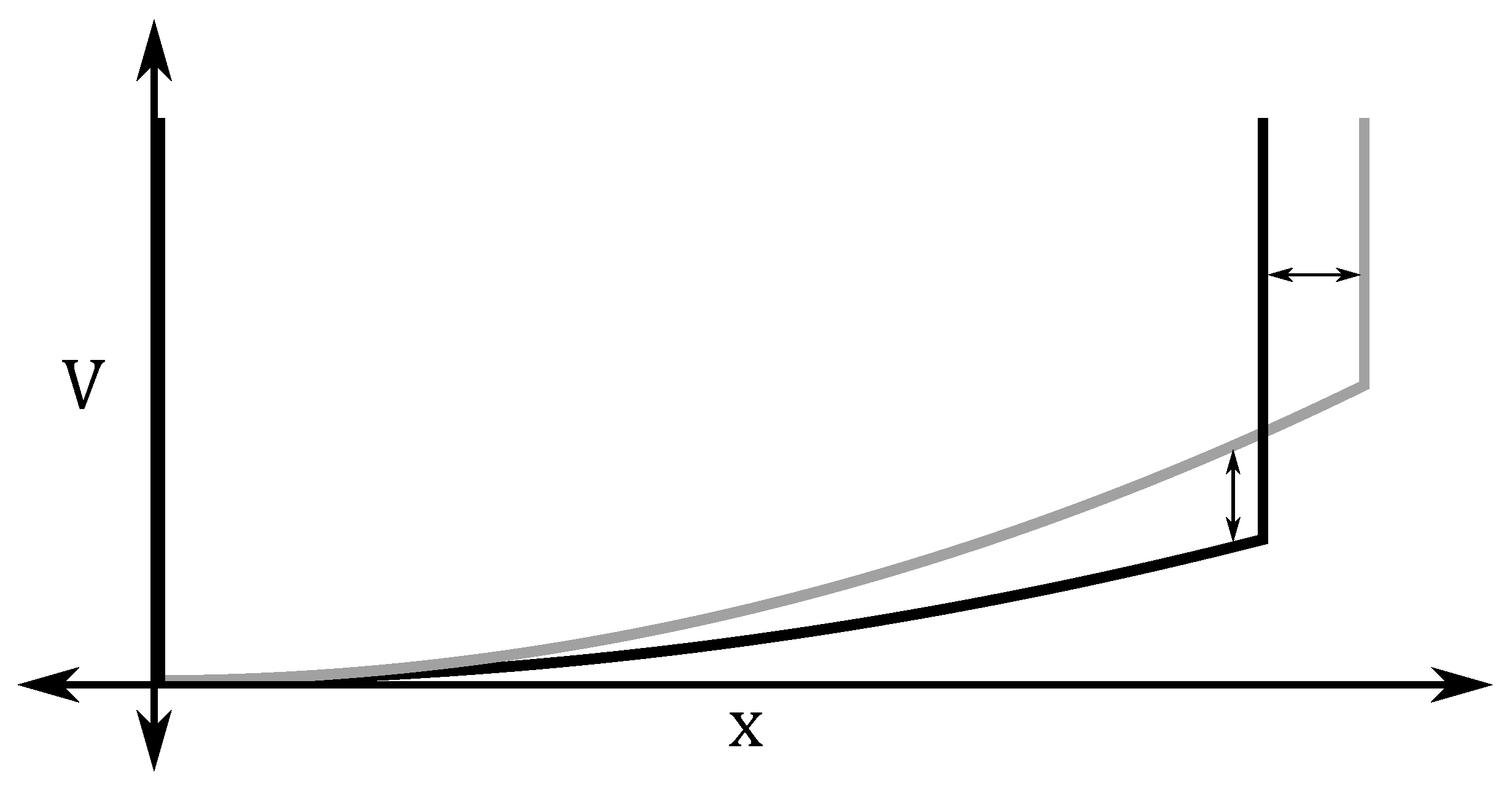
Figure 1.
Confined harmonic oscillator with the harmonic frequency and the position of the left wall periodic functions of time.
Figure 1.
Confined harmonic oscillator with the harmonic frequency and the position of the left wall periodic functions of time.

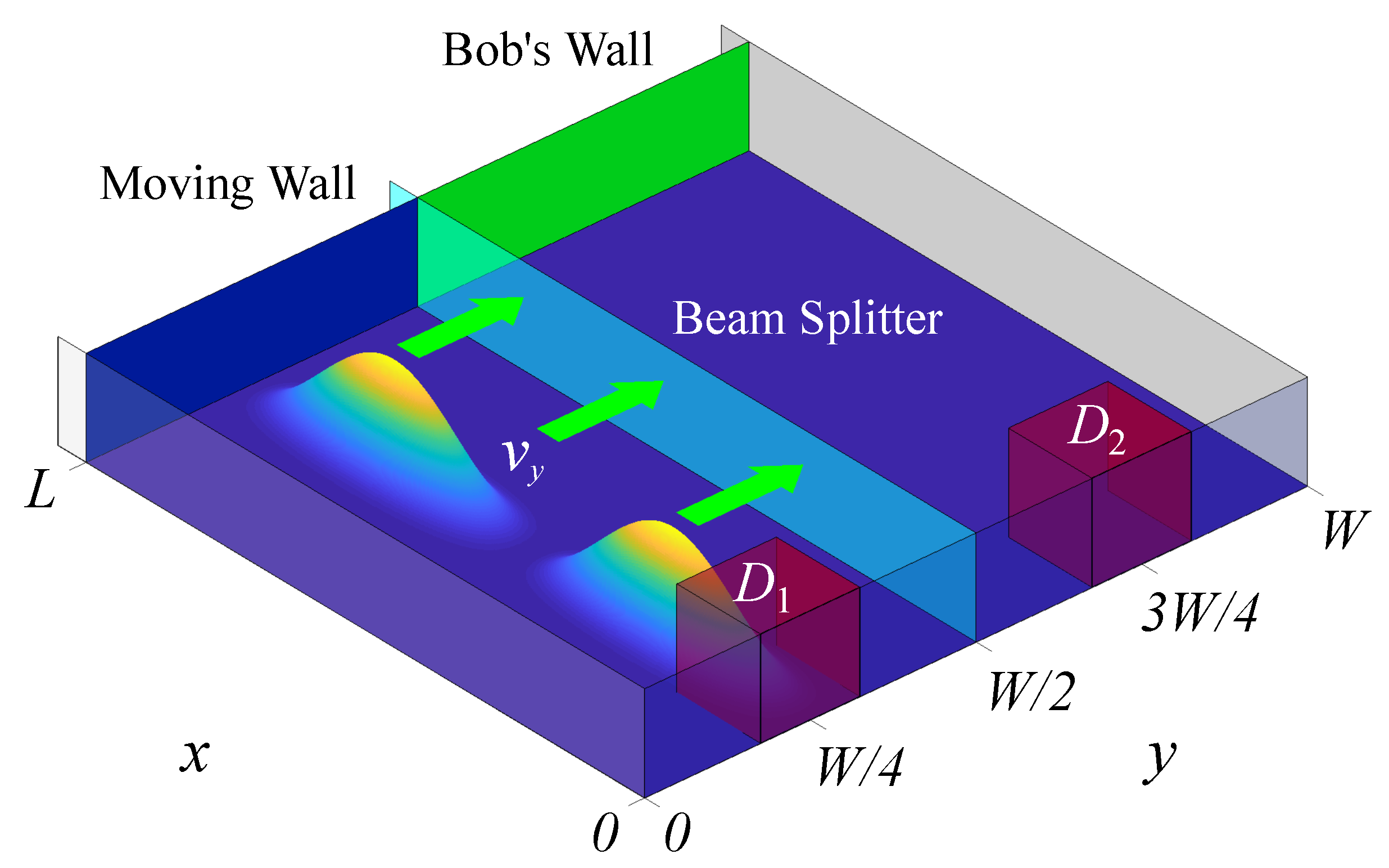
Figure 2.
A thought experiment allowing communication via the nonlocal phase of the wavefunction. The walls of the cavity are initially at rest, the harmonic potential is turned off, and the detectors are not yet in place. The particle begins in the state , where is an excited x-mode of the cavity ( is depicted), and is a narrow Gaussian initially centered at with average velocity . When the packet has divided at the beam splitter, the harmonic potential is turned on throughout the cavity, and the wall segment at begins to move as . At the same moment, Bob chooses whether the wall segment at begins to move as (Message 0) or (Message 1). The two half-packets propagate along y, then bounce off their respective walls and meet back at the beam splitter, a period after they left it. Bob choosing results in perfect interference, so the entire pulse recombines on the side of the beam splitter, whereas choosing results in a phase difference so that the interference is no longer perfect. Alice can detect Bob’s choice at by inserting detector at and detector at and measuring the relative intensity for the entire ensemble of cavities. , , and are all periodic function of time, with period T.

Figure 3.
Time evolution of the coefficients of Equation (16) in the adiabatic case, corresponding to the Hamiltonian given by Equations (29) and (30) with the following parameters: , (verifying where c is the light velocity). The initial state is . The thick solid blue line represents the numerically computed values of while the inset shows the corrections to the adiabatic approximation stemming from exact numerical computations: for are represented by the blue dot-dashed, solid red, and dashed green curves, respectively. We use atomic units (), where is the fine structure constant and the unit of time corresponds to s.

Figure 4.
Same as Figure 3 in the nonadiabatic case. The Hamiltonian parameters are those given for Figure 3 except we set here (atomic units are used). The initial state is again . The coefficients are shown by the curves in thick solid blue (), dot-dashed (), solid red (), and green dashed (). The coefficients for are of smaller and decreasing magnitude.

Figure 5.
Phase difference at between the Case III and Case I cavities obtained from numerical computations. (Top) The Case III cavity is in the adiabatic regime (corresponding to the parameters given in Figure 3). Applying the analytical expression (32), the phase difference is constant and computed to be (Bottom) The Case III cavity is in a nonadiabatic regime (the parameters are those given in Figure 4). Note the phase difference is two orders of magnitude higher than in the adiabatic case. Atomic units are used (the length unit is the Bohr radius).

Figure 6.
The phase (blue dots) in the nonadiabatic case of Figure 4 obtained from the numerically computed wavefunction as the basis size increases (cf. Equation (16)). It is seen that states up to at least are necessary in order for the computed value of to converge. The solid red line represents , the phase increment in Case I. The quantity that displays nonlocality here is the phase difference between Cases III and I (the blue dots and the red line), .

Publisher’s Note: MDPI stays neutral with regard to jurisdictional claims in published maps and institutional affiliations. |
© 2020 by the authors. Licensee MDPI, Basel, Switzerland. This article is an open access article distributed under the terms and conditions of the Creative Commons Attribution (CC BY) license (http://creativecommons.org/licenses/by/4.0/).
Share and Cite
MDPI and ACS Style
Waegell, M.; Matzkin, A. Nonlocal Interferences Induced by the Phase of the Wavefunction for a Particle in a Cavity with Moving Boundaries. Quantum Rep. 2020, 2, 514-528. https://0-doi-org.brum.beds.ac.uk/10.3390/quantum2040036
AMA Style
Waegell M, Matzkin A. Nonlocal Interferences Induced by the Phase of the Wavefunction for a Particle in a Cavity with Moving Boundaries. Quantum Reports. 2020; 2(4):514-528. https://0-doi-org.brum.beds.ac.uk/10.3390/quantum2040036
Chicago/Turabian StyleWaegell, Mordecai, and Alex Matzkin. 2020. "Nonlocal Interferences Induced by the Phase of the Wavefunction for a Particle in a Cavity with Moving Boundaries" Quantum Reports 2, no. 4: 514-528. https://0-doi-org.brum.beds.ac.uk/10.3390/quantum2040036