Interaction between Different Kinds of Quantum Phase Transitions

Abstract

We employ two different Lipkin-like, exactly solvable models so as to display features of the competition between different fermion–fermion quantum interactions (at finite temperatures). One of our two interactions mimics the pairing interaction responsible for superconductivity. The other interaction is a monopole one that resembles the so-called quadrupole one, much used in nuclear physics as a residual interaction. The pairing versus monopole effects here observed afford for some interesting insights into the intricacies of the quantum many body problem, in particular with regards to so-called quantum phase transitions (strictly, level crossings).

1. Introduction

The Lipkin Model (LM) is a celebrated exactly solvable model for nuclear physics [1,2]. Given that it provides one with accessible exact solutions, it has proved to be of great utility in nuclear theoretical research for the purpose of assessing the validity and/or usefulness of variegated techniques that have been devised in order to study the multiple facets of the quantum many fermions problem [3].

Lipkin’s model is based on an SU2 algebra that is generated by special operators denominated quasi-spin operators (QSPO). The model possesses tractable exact solutions, which are to be compared with results encountered via diverse kinds of approximate theoretical techniques. A relevant Casimir operator emerges in the model that commutes with all the QSPO [1,2]. This Casimir operator has attached to it different multiplets. Only the multiplet associated with the unperturbed ground state deserves scrutiny.

In addition to serving as a test ground for assessing many body methodologies, the Lipkin model also has considerable value as a conceptual tool for the exploration of questions of principle related to the many-body problem. This is the sense in which our present discussion proceeds, because our treatment of competing quantum phase transitions below could be viewed as the addressing of a possibly new quantum phenomenon.

Cambiaggio and Plastino (CP) [4,5] proposed a simple Lipkin augmentation, from SU2 to SU2 × SU2, to treat the excited Lipkin-multiplets (or bands) and the pairing interaction responsible for superconductivity. The extension permitted the enactment, in quasi-spin language, of a BCS-like formulation [2] which is able, as stated above, to exactly mimic superconductivity, giving exact solutions. We have then an extension of the Lipkin model to a scenario endowed with a variable particle number. Note that in nuclear physics superconductivity often arises as well [2]. There, the pairing interaction is an important component of the residual nuclear interaction left after the Hartree–Fock mean field has been established [2,6,7]. In particular, a second important component of the nucleon–nucleon interaction is a quadrupole force [2].

In this effort, we wish to exactly examine the competition between the pairing interaction and a monopole force. This is doable if we combine the solvable Cambiaggio–Plastino (CP) model of the pairing interaction with the also solvable Plastino–Moskowski (PM) model of a monopole interaction [8,9]. In particular, the two models display phase transitions (PT) and we show how the two PTs mutually interfere one with the other. The exactly solvable juxtaposition of the CP and PM models that we advance in this paper offers rich structural quantum details that deserve our attention.

2. Our Present CP-PM Juxtaposition

2.1. Preliminaries

We appeal to two different exactly solvable Hamiltonians of the Lipkin type ([10] and references therein), which we here juxtapose for the first time. The first is the Hamiltonian $H_{PM}$ of [9] (see (11) below), which represents forward scattering, spin-flips, or monopole interactions [9]. The second is the pairing Hamiltonian (15) below. The total $H=H_{PM}+H_{CP}$, representing monopole plus pairing interactions, here operates on an augmented SU2 × SU2 mathematical scenario.

One considers here N fermions distributed in two (2 $\Omega$)-fold degenerate single-particle levels (N = 2 $\Omega$) separated by an energy gap $ϵ$. All energies here are expressed in $ϵ$-units. The 4 $\Omega$ single particle states are characterized by two quantum numbers: (1) $p,\mu$ with $p=1,\dots$, 2 $\Omega$; and (2) $\mu =\pm 1$. p is named a quasi-spin quantum number. We appeal now to the customary fermionic creation ($C_{p,\mu }^{†}$) and destruction ($C_{p,\mu }$) operators. Creation (destruction) operators anti-commute among themselves. Additionally,

$$\{C_{p,\mu },C_{p^{\prime },{\mu }^{\prime }}^{†}\}={\delta }_{p,p^{\prime }}\delta \mu ,{\mu }^{\prime }.$$

(1)

One has then to deal with the usual SU2 quasi-spin operators [1,2], with which one constructs the pertinent Hamiltonians:

$$J_z=(1/2)\sum _{p,\mu }{C}_{p,\mu }^{†}{C}_{p,\mu },$$

(2)

$$J_{+}=\sum _p{C}_{p,+}^{†}{C}_{p,-},$$

(3)

$$J_{-}=\sum _p{C}_{p,-}^{†}{C}_{p,+}.$$

(4)

$J_z$ counts the difference between the number of particles in the upper level and that of the lower one. $J_{+}$ creates a particle upstairs while destroying one below, and vice versa for $J_{-}$. These two operators move fermions up and down. Its authors introduced the (also SU2) angular momentum-like “pairing” entities [4]

$$Q_0=\frac{1}{2}\sum _{p,\mu }{C}_{p,\mu }^{†}{C}_{p,\mu }-\Omega ,$$

(5)

$$Q_{+}=\sum _p{C}_{p,+}^{†}{C}_{p,-},$$

(6)

$$Q_{-}=\sum _p{C}_{p,-}^{†}{C}_{p,+}.$$

(7)

It is evident that $Q_{+}$ creates and $Q_{-}$ destroys two particles, yielding null bequest to the $J_z$-value, and one then shows that the two particles couple to $J_z=0$. Any Q-operator does commute with all J-operators, and the other way around, which entails an SU2 × SU2 structure. We can construct then a complete orthonormal basis characterized by the eigenvalues of the operators $J^2,J_z,Q^2,Q_0$, i.e., $|J,Q,J_z,Q_0\rangle$. CP [4] also introduces the quasi-spin seniority number $\nu$

$$\nu =2(\Omega -Q),$$

(8)

which reveals the number of particles not “paired” to $J_z=0$. Thus, $\nu$ is the quantity of “unpaired” particles in a Q-multiplet. Note that one has [4]

$$J=\nu /2,$$

(9)

$$J+Q=\Omega .$$

(10)

In the Lipkin model, N = 2 $\Omega$, $Q_0=0$ [1,4], and this equality is strictly obeyed in all what follows below.

The unperturbed ground state is the eigenvalue of an unperturbed Hamiltonian $H_0$ (no fermion–fermion interaction) and is characterized by $J=\Omega ,J_z=-\Omega ,Q=Q_0=0$ [4] belonging to the multiplet $J=\Omega ,Q=Q_0=0.$

We consider now that the monopole Hamiltonian $H_M$ in our scenario. We have, as defined in [9], in terms of the operators J and $J_z$ and a coupling constant V,

$$H_{PM}=H_0+H_M=H_0-V\left[J^2-J_z^2-J\right],$$

(11)

$$H_0=J_z.$$

(12)

The exact eigenvalues of $H_{PM}$ are immediately seen to be [9]

$$E(J,Q,J_z,Q_0)=J_z-V\left[J^2-J_z^2-J\right].$$

(13)

The energy of the unperturbed ($V=0$) ground state ($\nu =N,Q=Q_0)$ is

$$E_0=-\Omega .$$

(14)

As V grows, this Hamiltonian displays $\Omega$ phase-transitions (level crossings) in which the ground state ceases to be characterized by $J_z=-J$ and passes to be characterized by successively larger $J_z$ values until we reach $J_z=0$ at $V=1$ [9]. This assertion is immediately verified by inspection.

A second, pairing interaction, is now added to our PM–CP picture [4] as

$$H_{CP}=H_0-\frac{G}{2}{\widehat{Q}}_{+}\left(b\right){\widehat{Q}}_{-}\left(b\right),$$

(15)

which adds to the energy a pairing amount $E_p$

$$E_P=-(G/2)Q(Q+1).$$

(16)

A superconducting phase transition takes place at $G=G_{crit}$ [4] (this fact can be easily verified by analytically computing ground state energies)

$$G_{crit}=\frac{2}{\omega +1}.$$

(17)

Our pairing contribution to the total Hamiltonian is thus

$$H_{CP}=-\frac{G}{2}{\widehat{Q}}_{+}\left(b\right){\widehat{Q}}_{-}\left(b\right).$$

(18)

The Hamiltonian $H_0+H_{CP}$ exhibits a phase transition (level crossing) at $G=1$ from non-conducting to superconducting. At such value, the system becomes a superconductor, as can be immediately verified [4].

In this paper, we wish to ascertain what happens to our two kinds of phase transitions (pt) in the case of the juxtaposition total Hamiltonian

$$H=H_0+H_M+H_{CP}.$$

(19)

In other words, we want to see

• how the monopole pt depends on the pairing coupling constant G; and
• how the superconducting pt depends on the monopole coupling constant V.

2.2. Statistical Mechanics of the Combined Hamiltonian H

How to statistically handle H is described in [11]. For investigating ground states, only the $J+Q=\Omega$ “band” requires attention at temperature $T=0$. If $T>0$, the picture changes. For non-zero temperatures, plenty of states belonging to other bands become accessible (double p occupancy is now allowed for), as we construct the pertinent statistical ensemble. Define then the degeneracy $Y(J,Q)$ of a given multiplet defined for specific values of the quantum numbers Q and J. This is a rather involved task. One has [11] ($\beta$ is the inverse temperature $1/T$)

$$Y(J,Q)=\frac{(2\Omega +2)!(2\Omega )!(2J+1)(2\Omega +1)}{(\Omega +J+Q+2)!(\Omega +J-Q+1)!(\Omega -J+Q+1)!(\Omega -J-Q)!}.$$

(20)

A partial partition function $Z_M$ can be written as $Z_M$ [11]

$$Z_M\left(\beta \right)=\sum _{M=-J}^{M=J}exp[-\beta [(M-V[J^2-M^2-J])-(G/2)Q(Q+1)].$$

(21)

The system’s total partition function Z is now

$$Z\left(\beta \right)=\sum _{J,Q}Y(J,Q)Z_M\left(\beta \right),$$

(22)

where J and Q run over all the quantum numbers allowed for by the structural SU2 × SU2 restrictions [11]:

$$0\le J\le \Omega ,$$

(23)

$$0\le Q\le \Omega ,$$

(24)

$$0\le J+Q\le \Omega .$$

(25)

Naturally, once in possession of Z, all relevant statistical quantifiers become easily obtainable.

Two very important quantities are

• The effective superconductivity index X,

  $$X=\sum _{J,Q}\sum _{M=-J}^{M=J}P(M,Q)[(N-\nu )/N],$$

  (26)

  is unity for a perfect superconductor and vanishes for the unperturbed system (no pairing interaction).
• Its equivalent quantity for the monopole force (the monopolarity indicator W) is

  $$W=\sum _{M=0}^{M=J}P(M,Q=0,J=\Omega ).$$

  (27)

3. Results

We deal in this work with two competing interactions, a monopole one, which mimics a long range interaction [9], and a pairing one, which mimics short range ones [4].

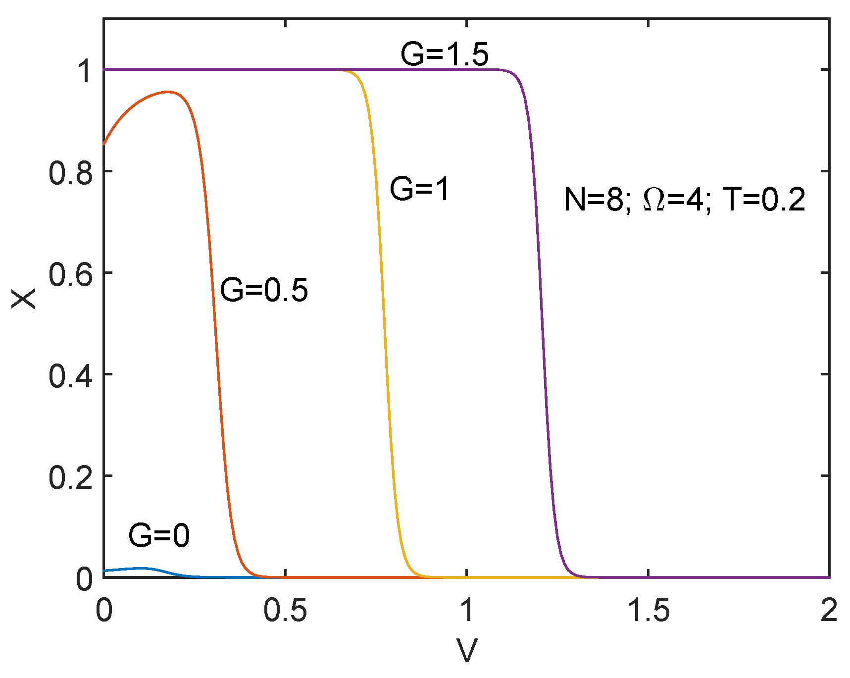
We illustrate the rather surprising influence that the monopole interaction has on pairing in Figure 1. Since $T\ne 0$, there is some superconductivity even at $G<G_{crit}$ [5]. The notable result is that growing V either helps or impedes superconductivity, according to the surrounding circumstances, an original discovery of ours here. Recall that, at $T=0$, the monopole interaction generates, at $V=V_{crit}=1$, a monopole phase transition [9]. The helping “V” effect takes place if $V<V_{crit}$. Contrariwise, the “impeding” effect prevails.

Figure 1 refers to the special case $N=2$. Here, the influence of the monopole interaction always favors pairing. This changes for larger N values, as shown below.

A new facet of the interplay between the monopole and pairing interactions is shown in Figure 2 for $N=8$. One appreciates the following fact. Little V-values, i.e., smaller than $V_{crit}$, help pairing, but great ones, i.e. larger than $V_{crit}$, tend to destroy it. In this example, pairing dies for $V>1.35$. We see a sort of interaction between the two different phase transitions at play here.

Figure 3 is a three dimensional picture in which X is called H. It is plotted versus V and G for $N=8$. At $G=2$, pairing vanishes for $V_{terminal}=1.8$. $V_{terminal}$ describes a straight line at the graph’ floor from that value to near $V=0.5$. Here downwards, V reverses its impeding role and begins instead to help pairing. This happens as, diminishing its value, V crosses $V_{crit}$ downwards. Thus, the physics of the monopole phase transition determines the monopole role in helping or preventing superconductivity. We emphasize the remarkable feat that the monopole interaction destroys pairing if intense enough. This can be easily understood: in actual nuclei, the residual quadrupole force is a long-range one while pairing is short-range. Thus, it is understandable that the former works against the latter.

3.1. The N-Dependence

As shown above, the superconducting state suddenly emerges whenever the coupling constant G, when growing from zero, reaches a critical value $G_{crit}$. This critical value is roughly proportional to $1/N$. Instead, the critical constant $V_{crit}$ is independent of N.

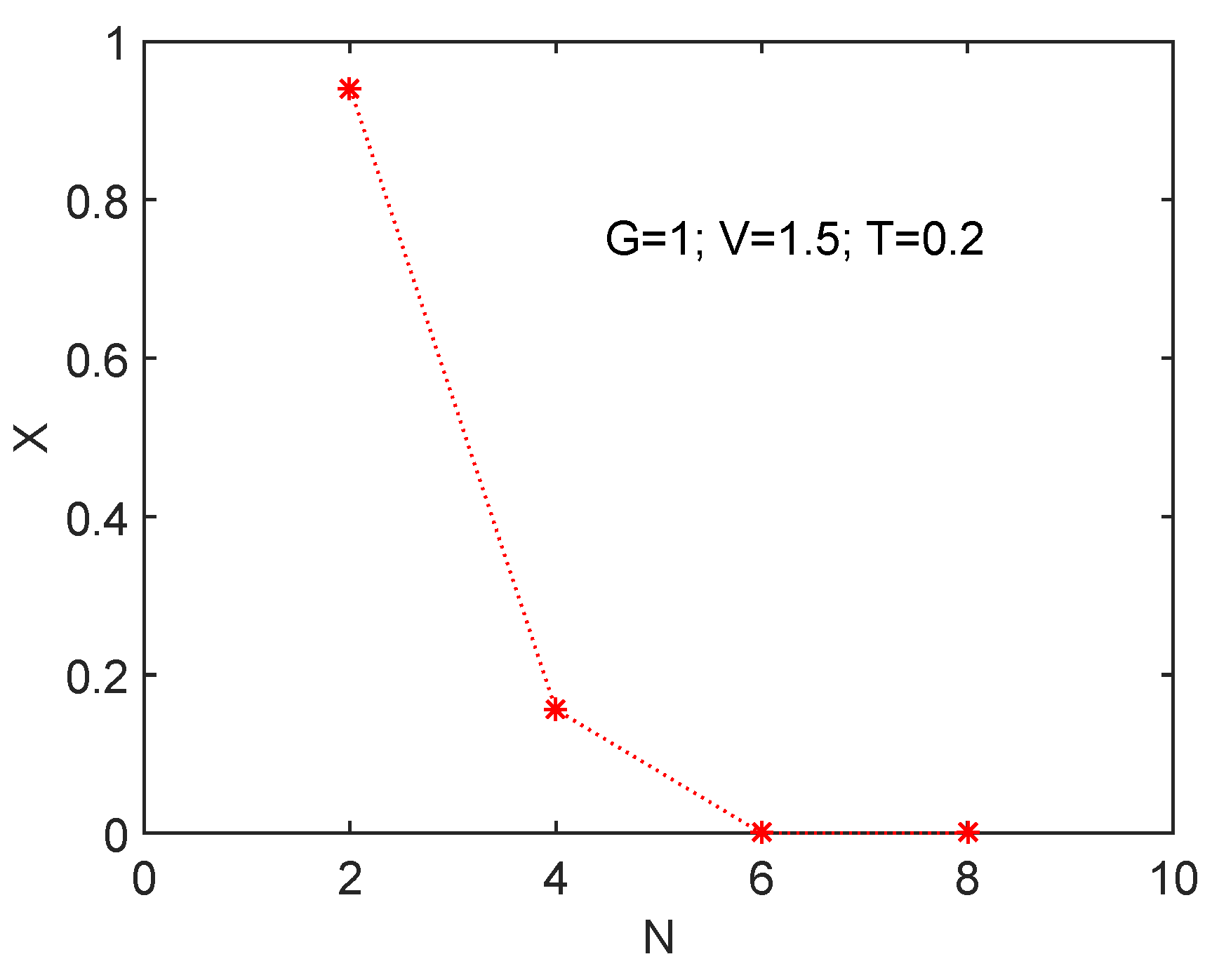
The N dependence is analyzed next in Figure 4. This is of the essence, as the effects of a long range interaction should obviously gain intensity as N grows. As a consequence, for $V>V_{crit}$, its pairing impeding role becomes stronger. This is clearly shown in Figure 4. Pairing effects are attenuated as N augments.

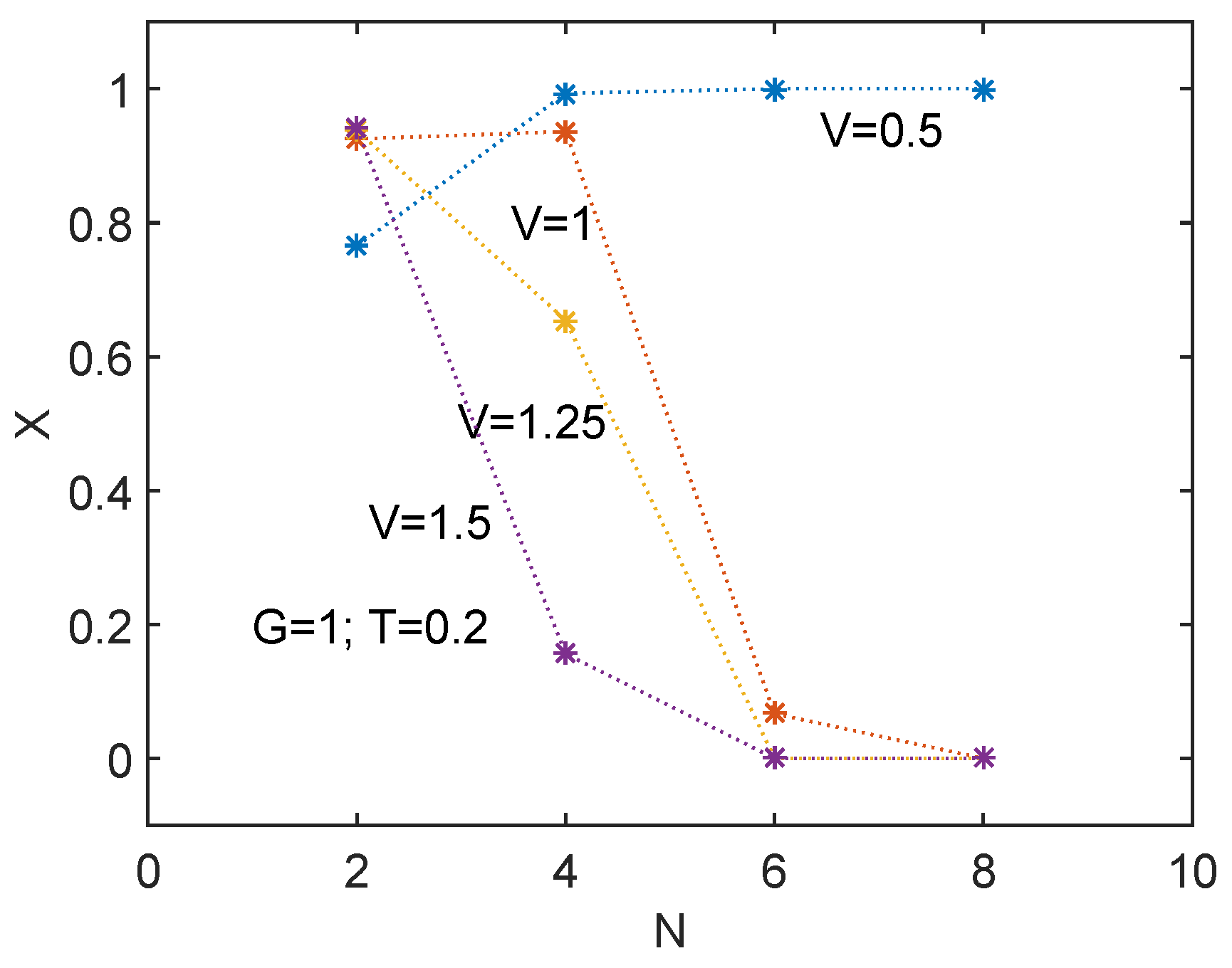
As noted above, however, the N dependence, in turn, hinges upon whether the V value is large or small. This is illustrated in Figure 5. V small helps pairing and V large impedes it.

As stated above, the N dependence of pairing hinges upon whether the V value is large or small. This is illustrated in Figure 6 by plotting X versus V for several N values.

3.2. The Monopole-Intensity Quantifier W

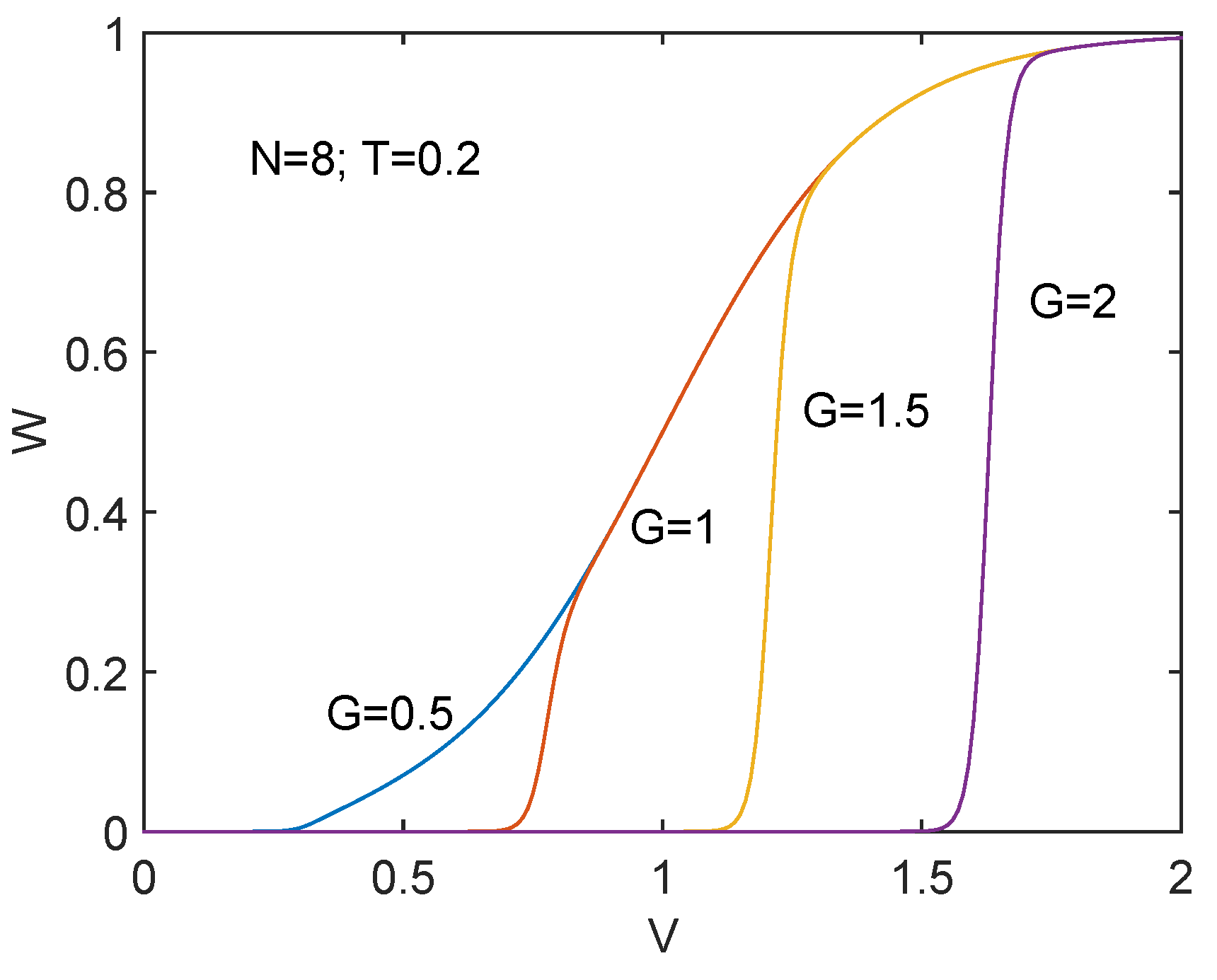
We focus attention now on the monopole-intensity quantifier W and study how pairing impinges on it. Figure 7 shows that pairing tries to impede the monopole force action.

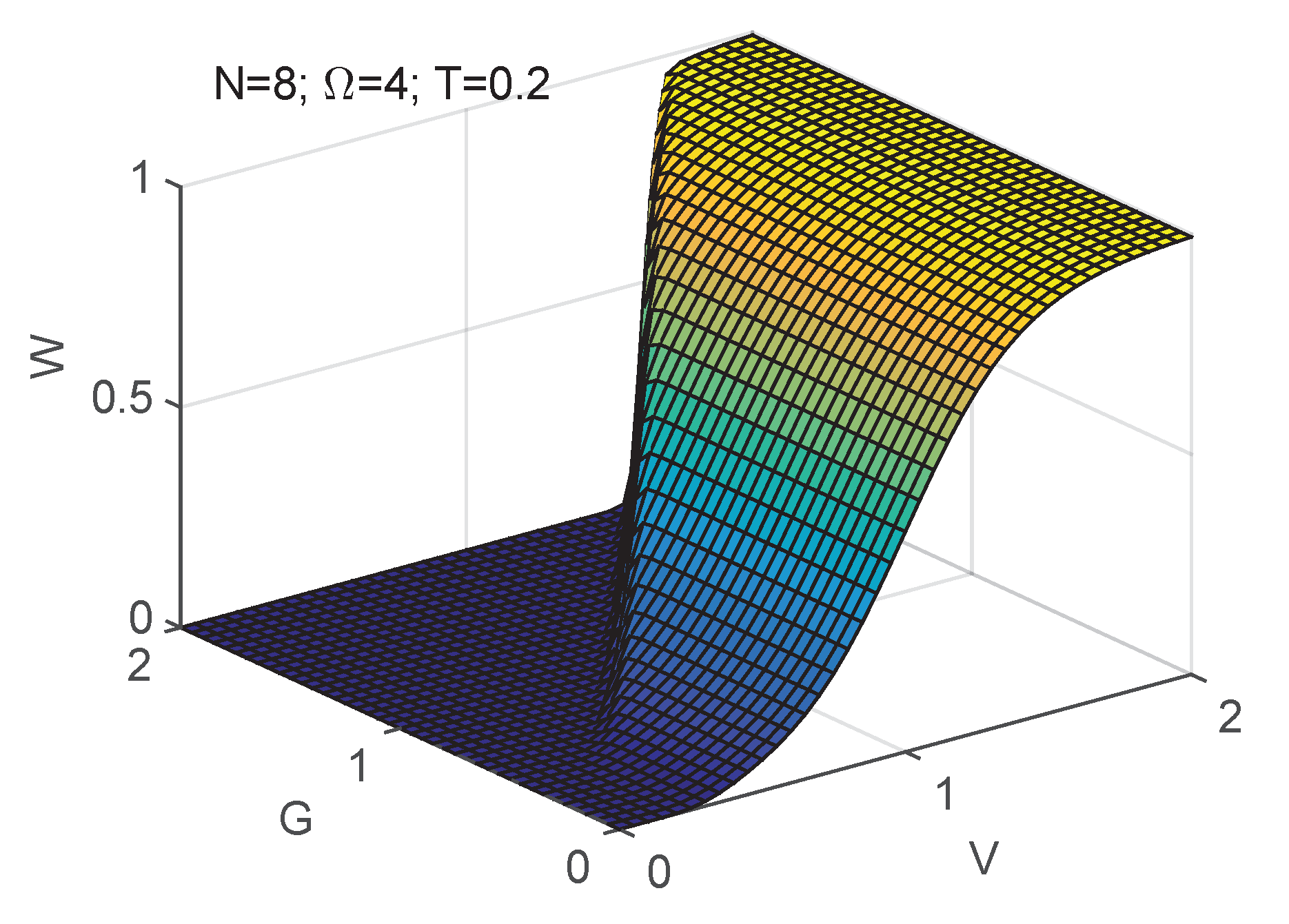
We maintain our focus on the monopole-intensity quantifier W and consider in Figure 8 a 3D plot in which W is depicted against both V and G for $N=8$ and $T=0.2$. We see that pairing tries to impede the monopole force action.

4. Conclusions

This paper shows how different fermion–fermion interactions compete against each other in a novel juxtaposition of two exactly solvable many-fermion systems, those found in [4,9]. Both are endowed with phase transitions (level crossings) of distinct kinds that mutually influence each other, either favorably or unfavorably, according to whether the pertinent coupling constant are smaller or larger than their respective critical values.

All the interesting effects described above in some detail are the result of a simple fact: as their respective coupling constant grows, the concomitant two fermion–fermion interactions try to ”drive” the system towards radically different types of states. The monopole force favors states in which each p-quasi-spin site is of a particle-hole character, of the total $J_z$ null-value. The pairing force tends to realize states in which each p-quasi-spin site is either empty or doubly occupied. The different tendencies freely compete here. The results depend on the values adopted by the two coupling constants V and G. Interesting results ensue, which we describe above.

References

- Lipkin, H.J.; Meshkov, N.; Glick, A.J. Validity of many-body approximation methods for a solvable model: (I). Exact solutions and perturbation theory. Nucl. Phys. 1965, 62, 188–198. [Google Scholar] [CrossRef]
- Ring, P.; Schuck, P. The Nuclear Many-Body Problem; Springer: Berlin/Heidelberg, Germany, 1980. [Google Scholar]
- Nolting, W. Fundam. Many-Body Physics; Springer: Berlin/Heidelberg, Germany, 2009. [Google Scholar]
- Cambiaggio, M.C.; Plastino, A. Quasi spin pairing and the structure of the Lipkin Model. Z. Phys. A 1978, 288, 153–159. [Google Scholar] [CrossRef]
- Pennini, F.; Plastino, A. Complexity and disequilibrium as telltales of superconductivity. Phys. A 2018, 506, 828–834. [Google Scholar] [CrossRef]
- De Llano, M.; Tolmachev, V.V. Multiple phases in a new statistical boson fermion model of superconductivity. Phys. A 2003, 317, 546–564. [Google Scholar] [CrossRef]
- Uys, H.; Miller, H.G.; Khanna, F.C. Generalized statistics and high-Tc superconductivity. Phys. Lett. A 2001, 289, 264–272. [Google Scholar] [CrossRef] [Green Version]
- Plastino, A.; Ferri, G.L.; Plastino, A.R. Spectral explanation for statistical odd-even staggering in few fermions systems. Quantum Rep. 2021, 3, 166–172. [Google Scholar] [CrossRef]
- Plastino, A.; Moszkowski, S.M. Simplified model for illustrating Hartree-Fock in a Lipkin-model problem. Nuovo Cimento 1978, 47, 470–474. [Google Scholar] [CrossRef]
- Debergh, N.; Stancu, F. The Lipkin–Meshkov–Glick Model and its Deformations through Polynomial Algebras. Proc. Inst. Math. NAS Ukr. 2002, 43, 432–438. [Google Scholar]
- Rossignoli, R.; Plastino, A. Thermal effects and the interplay between pairing and shape deformations. Phys. Rev. C 1985, 32, 1040. [Google Scholar] [CrossRef] [PubMed]
Figure 1.
Superconductivity indicator X versus monopole coupling constant (cc) V for various values of the paring cc G. We have and Remember that the pairing’s cc at is .
Figure 2.
Superconductivity indicator X versus monopole coupling constant (cc) V for various values of the paring cc G. We have and . Intense monopole forces destroy pairing.
Figure 3.
Superconductivity indicator versus monopole coupling constant (cc) V and pairing force cc G. We have and . Intense monopole forces destroy pairing. Weak ones, instead, favor it.
Figure 4.
The N dependence. Superconductivity indicator X versus N for (greater than ) and pairing force (the critical one at ). We have here. The pairing effects’ intensity abruptly falls as N grows.
Figure 5.
The N dependence. Superconductivity indicator X versus N for several V values. We have . The pairing effects’ intensity falls or grows as N grows, according to how large V is—more precisely, according to whether it is greater or smaller than .
Figure 6.
The N dependence. Superconductivity indicator X versus V for several N values. The larger is N, the sooner does V destroy pairing.
Figure 7.
The N dependence. Monopole activity-indicator W versus V for several G values. and . Growing pairing works against W.
Figure 8.
3D study. The N dependence. Monopole activity-indicator W versus V and versus G. and . Growing pairing works against W, more strongly for .
Publisher’s Note: MDPI stays neutral with regard to jurisdictional claims in published maps and institutional affiliations. |
© 2021 by the authors. Licensee MDPI, Basel, Switzerland. This article is an open access article distributed under the terms and conditions of the Creative Commons Attribution (CC BY) license (https://creativecommons.org/licenses/by/4.0/).
Share and Cite
MDPI and ACS Style
Plastino, A.R.; Ferri, G.L.; Plastino, A. Interaction between Different Kinds of Quantum Phase Transitions. Quantum Rep. 2021, 3, 253-261. https://0-doi-org.brum.beds.ac.uk/10.3390/quantum3020015
AMA Style
Plastino AR, Ferri GL, Plastino A. Interaction between Different Kinds of Quantum Phase Transitions. Quantum Reports. 2021; 3(2):253-261. https://0-doi-org.brum.beds.ac.uk/10.3390/quantum3020015
Chicago/Turabian StylePlastino, Angel Ricardo, Gustavo Luis Ferri, and Angelo Plastino. 2021. "Interaction between Different Kinds of Quantum Phase Transitions" Quantum Reports 3, no. 2: 253-261. https://0-doi-org.brum.beds.ac.uk/10.3390/quantum3020015