1. Introduction
Stream flow forecasting plays an important role in environmental and hydrological research and disaster management. Nowadays, mathematical models are emerging for more precise and longer-horizon daily reservoir inflow forecasting that can be beneficial for reservoir operation, flood warning, and optimal water allocation for various water users. Predicting peak flows can help us to control floods and hydropower operation.
One of the successful mathematical forecasting models are autoregressive models such as Autoregressive Integrated Moving Average (ARIMA) and multilayer perceptron Artificial Neural Network (ANN). Autoregressive models forecast future values of time series based on the identification of past temporal patterns of the records. The main hypothesis of ARIMA models, which are conventional forecasting models, assumes a linear relationship between historical time series for the forecasting of future variables [
1]. Hence, ARIMA models cannot forecast the nonlinear pattern of inflow time series. On the other hand, ANN models, as well-known forecasting models, are able to model nonlinear time series [
1]. Autoregressive forecasting models can be categorized based on their time horizon as short-term, mid-term, and long-term which are from a part of a day to a week, weeks up to a month, and months to years, respectively. Applied time scales for inflow forecasting are hourly, daily, weekly, monthly, quarterly, and yearly [
2,
3,
4,
5,
6,
7]. One of the advantages of machine learning models is to forecast time series for long-term horizons. Recently, many studies reported the need for forecasting daily hydrological data at a long-term horizon (at least for one year ahead) [
8,
9,
10,
11,
12].
Some ANN models are linked with conventional auto-regressive models (Auto Regressive (AR) and ARIMA) to reveal their ability in short-term horizon forecasting of daily flow. Kisi and Cigizoglu [
3] used Feed-Forward Artificial Neural Network (FF-ANN) and AR models to forecast daily flow for three rivers in the USA and a river in Turkey. Three artificial neural network structures were then selected for comparison with the AR model forecasts. Given the same input data for 1-day-ahead forecasts, the results showed that ANN structures were able to produce better results than AR models. Banihabib et al. [
2] forecasted the daily inflow to the Dez reservoir by using an FF-ANN model and a linear regression model based on inflow data from hydrometric stations located upstream of River Dez. The research showed that in short-term horizon forecasting, the FF-ANN performed better than linear regression models. Xie [
13] used linear regression and exponential smoothing ANN models to forecast daily flow. These models performed well during the dry seasons while the non-linear ANNs were superior to the other models in forecasting flood flows of rainy seasons; however, they still had limitations in forecasting peak flows [
13]. Sattari et al. [
14] forecasted daily flow upstream of Eleviyan Reservoir by a Recurrent ANN (RANN) and a Back-Propagation Neural Network (BP-NN). The results suggested that both models are fair in one-day ahead forecasting of flood flow. However, both models performed well when they were applied for forecasting low flows. Consequently, these studies show that ANN models perform better for a short-term horizon forecasting of daily low flow. However, even for the short-term horizon forecasting of inflow, ANN models do not have a considerable accuracy for peak flows such as flood flows.
Several ARIMA and Artificial Neural Network (ANN) models are proposed for forecasting of inflow in monthly, quarterly, and yearly time scales [
4,
5,
6,
15,
16,
17,
18,
19,
20], while autoregressive models are reported for successful forecasting of daily flow at short-term time horizons [
2,
3,
14,
21,
22,
23,
24,
25,
26]. The forecasting horizon of most of short term autoregressive models are only one day or 3- to 7-days ahead of flow forecasting [
2,
3,
6,
21,
23,
24,
25,
27]. These short-term horizon flow forecasting can benefit single-purpose dam for the purpose of flood control. However, a longer horizon of forecasting is required for optimal operation of a multi-purpose dam that provides water for hydropower generation, flood control, domestic water supply, and irrigation. There are other successful investigations of daily forecasting for at least one year ahead [
8,
10,
11,
12]. Banihabib et al. [
9] proposed a non-linear auto-regressive ANN model for forecasting daily streamflow for a long-term horizon versus an ARIMA model. The auto-regressive ANN model improved long-term forecasting daily streamflow by continuously following a daily flow pattern compared to the ARIMA. However, the proposed model has still considerable uncertainty in forecasting peak flows.
The literature review indicates that developing autoregressive models are needed to forecast daily reservoir inflow, especially peak flows for a long-term horizon, to provide the optimal operation of multi-purpose reservoirs for flood control, hydropower generation, domestic water supply, and irrigation purposes. Since forecasting by regular ANN has already been done [
2,
6,
9], we focused on using hybrid ANN models in this study to keep a novelty aspect of the work, as well as to increase the accuracy of the predictions. Indeed, the novelty of this research compared to previous studies like Banihabib et al. [
9] is developing a hybrid autoregressive model (a combination of linear and nonlinear forecasting models) to present a robust forecasting model for peak flows in long-horizon daily reservoir inflow forecasting.
The results of this study are applicable for stakeholders and water resources managers to schedule optimum operation of multi-purpose reservoirs to control floods and to generate optimum hydropower.
2. Materials and Methods
2.1. Multi-Purpose Reservoir and Reservoir Inflow Data
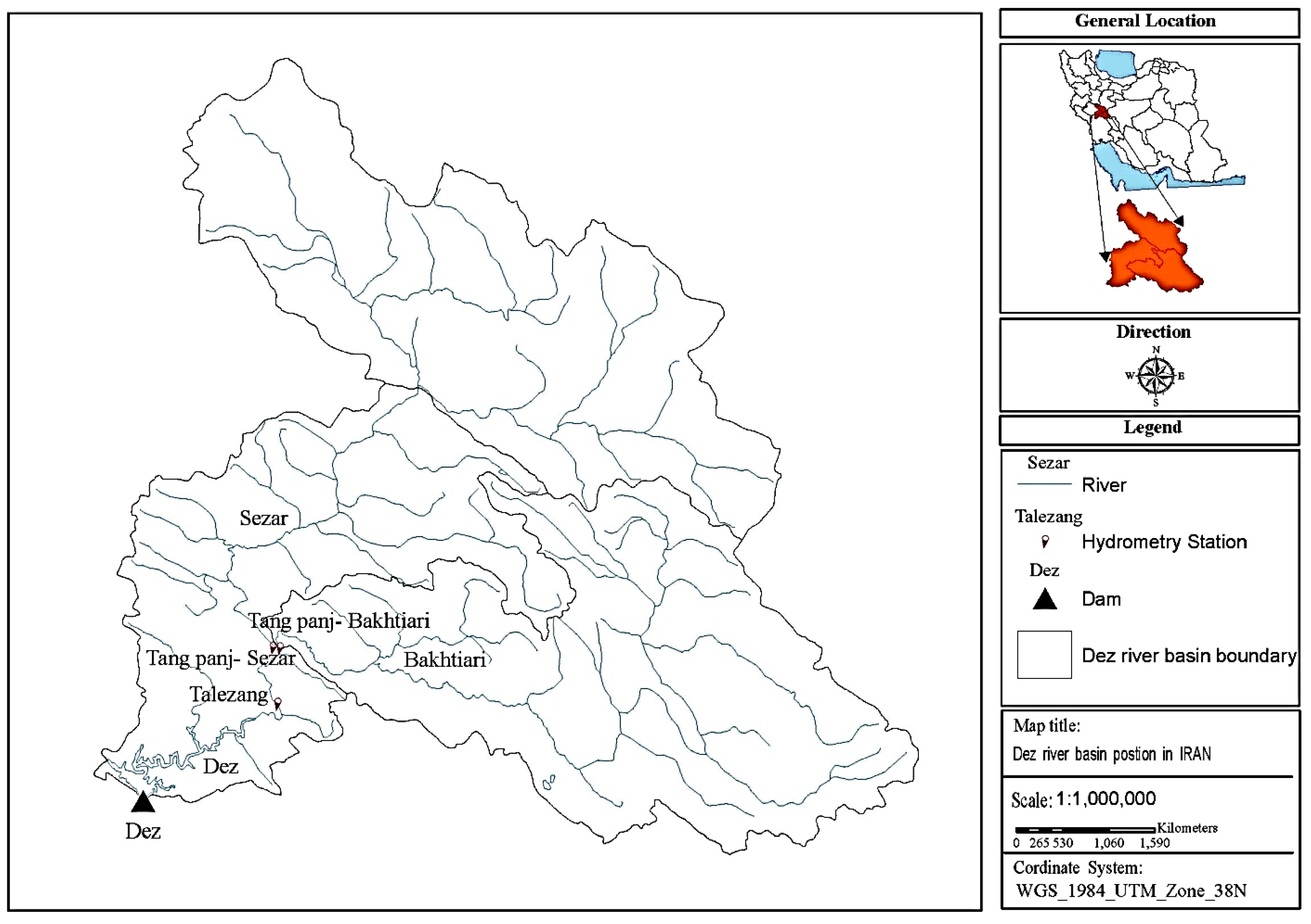
To examine the performance of the proposed autoregressive hybrid model, a multi-purpose reservoir (Dez Dam) has been selected as a case study.
Figure 1 shows the location of the Dez basin. The reservoir aims to control floods, generate hydropower, and supply agricultural and domestic water. The Dez reservoir basin is at a latitude of 32°35′N to 34°07′N and longitude of 48°20′ to 50°20′E in Southwest Iran. In this research, the daily flow records of Taleh-Zang hydrometric station located upstream of the reservoir were used to forecast inflow to the reservoir. In addition, daily discharge data from 1975 to 2011 of the hydrometric station were used for calibration/training and forecasting daily reservoir inflow. The dataset comprised 13,140 data points from 23 September 1975 to 22 September 2011. The data set was then split into two subsets. The daily stream flow from 23 September 1975 to 22 September 2010 was chosen for training (calibration), and daily reservoir inflow from 23 September 2010 to 22 September 2011 was chosen for forecasting. Access to the dataset can be requested by contacting the authors.
2.2. Overview of the Research Method and Performance Evaluation
The proposed hybrid autoregressive model consists two sub-models: Fourier Series Filtered ARIMA (FSF-ARIMA) for the linear part and RANN for the nonlinear part. Both sub-models have two processing phases: training (calibration), in which the models use historical observed inflow data for learning and then for forecasting (in which the models forecast the daily reservoir inflow for one year). First, FSF-ARIMA models were calibrated and used for forecasting the linear part of the reservoir inflow data, then the RANN model was trained and used for forecasting the non-linear part of the data.
In this study, reservoir inflow forecasting was carried out by using a conventional model (FSF-ARIMA model) and the proposed model (autoregressive hybrid model), and the results were compared with evaluation indices. Through comparing the models with observed data, the performance of each model was assessed in daily reservoir inflow forecasting. Error Index (EI) and coefficient of determination (
) were employed as the indices for performance evaluation of the autoregressive hybrid and FSF-ARIMA models in training and forecasting phases as below [
2,
6,
9]:
where
and
are the forecasted and observed daily reservoir inflow in the
th day of the forecasting horizon, and
is the number of data points.
is the average of observed reservoir inflow. The training phase contains 12,775 data points and
is 262 m
3/s. The forecasting phase comprises 365 data sets where
equals to 141 m
3/s.
In the forecasting phase, to compare the one-year observed inflow hydrograph with the forecasted hydrographs of the models,
,
, and Average Cumulative Relative Error (
) are applied for performance evaluation of autoregressive hybrid and FSF-ARIMA models.
is defined for determining the best forecasting duration as follows [
2,
6,
9]:
where
is the average cumulative relative error until a certain month, and
is the cumulative number of days until that certain month.
is used to evaluate the time-tendency of error of the models in the forecasting phase.
In this study, we used Windows OS; programming language: MATLAB for RANN and R 2.13.0 for FSF-ARIMA. We stopped training when Mean Squared Error (MSE) was at the minimum. Training algorithm: Levenberg–Marquardt algorithm; number of hidden layers: 1; transfer functions of hidden layer: tangent-sigmoid (tansig) and log-sigmoid (logsig); transfer function in the output layer: pure line. We also tested 1760 nonlinear autoregressive network with exogenous inputs (NARX)-recurrent neural network (RNN) (NARX-RNN) model structures differing in transfer functions, numbers of inputs (2–5), and neurons per hidden layer (1–22); input delays and output delays ranged from 1 to 10. We tested two training algorithms: Levenberg–Marquardt (LM) algorithm and traingdx, but LM was applied as the learning function, finally, because it has generally high accuracy and it is fast learning.
2.3. Previous Linear and Nonlinear Models
To examine the capability of the proposed hybrid model, the previous linear and nonlinear models (FSF-ARIMA RANN models) proposed by Banihabib et al. [
9] were applied to the case study, and their results were compared to the result of the developed hybrid model.
The procedure for applying FSF-ARIMA to the seasonally variable reservoir inflow data for a one-year horizon is summarized as follows [
9]. The FSF-ARIMA procedure requires normally distributed stationary reservoir inflow time series. First, the time series are normalized using a logarithm transformation [
28]. This method has been successfully employed for inflow forecasting based on past investigations [
29,
30,
31]. Then the mean and standard deviation of the logarithm-transformed data are computed. In the next step, a Fourier Series was used to remove the seasonal tendency in the logarithm transformed time series [
1,
9]. The FSF-ARIMA(p,d,q) model is used (Equation (5)) to forecast daily stream flow data [
9]. Multiple FSF-ARIMA models were tried, and the most suitable model was selected using the Akaike Information Criterion (
) [
32] as a well-known criterion for evaluating time series models. The Fourier-transformed data is defined as below:
where
and
are the Fourier-transformed data and random error, respectively, at time step t.
(
i = 1, 2,…, p) and
(
j = 1, 2,…, q) are model parameters, p is the autoregressive model order, and q is the moving average model order [
33]. The FSF-ARIMA model with the best results based on
and the number of parameters was used for forecasting and determining the linear part of the steam flow data. Then
is forecasted using Equation (5) for one year ahead.
Several FSF-ARIMA(p,1,q) models are developed and values of p and q are determined based on minimization of
. For each candidate model, we use Equation (6) to compute the AIC as below:
Building RANN consists of selecting a learning function, inputs, and activation and training functions [
9]. The Levenberg–Marquardt (LM) algorithm was applied as the learning function, which has generally high accuracy and is fast learning [
34]. The neural networks involve bias, one hidden layer, and tangent-sigmoid or log-sigmoid as activation functions. A pure linear activation function was applied in the output layer. Besides, the appropriate number of output delays is determined by trial and error process.
2.4. The Proposed Autoregressive Hybrid Model
The proposed hybrid model benefits from the unique advantages of both autoregressive models, FSF-ARIMA, and RANN models, to recognize linear and nonlinear patterns of reservoir inflow time series. Both FSF-ARIMA and RANN models are autoregressive. Therefore, the hybrid model is also an autoregressive model. Developing the proposed hybrid model generally includes two steps. In the first step, an FSF-ARIMA model is applied to forecast linear elements of daily inflow time series. In the second step, a RANN model is employed to forecast FSF-ARIMA model residuals. Since FSF-ARIMA models cannot calculate nonlinear structures of the datasets, the residuals of the FSF-ARIMA model are the nonlinear part of the stream flow time series and can be forecasted by the nonlinear part of the proposed hybrid model (RANN). The Residuals of Linear Forecasting (
) can be computed as follows:
where
is output discharge. To forecast the nonlinear part of reservoir inflow time series (
), the proposed autoregressive hybrid model employs the RANN model. The RANN model is trained with
time series to find the following autoregressive nonlinear relation:
where
is a nonlinear function estimated using the RANN;
is the number of output delays and is tested for 1, 2, 3, 4, 5 in multiple RANN (RANN1 to RANN5); and
is the day of year of the forecasted day;
is the predicted flow at time step
.
is
-day delayed flow data (observed data in training and forecasted values in forecasting phase).
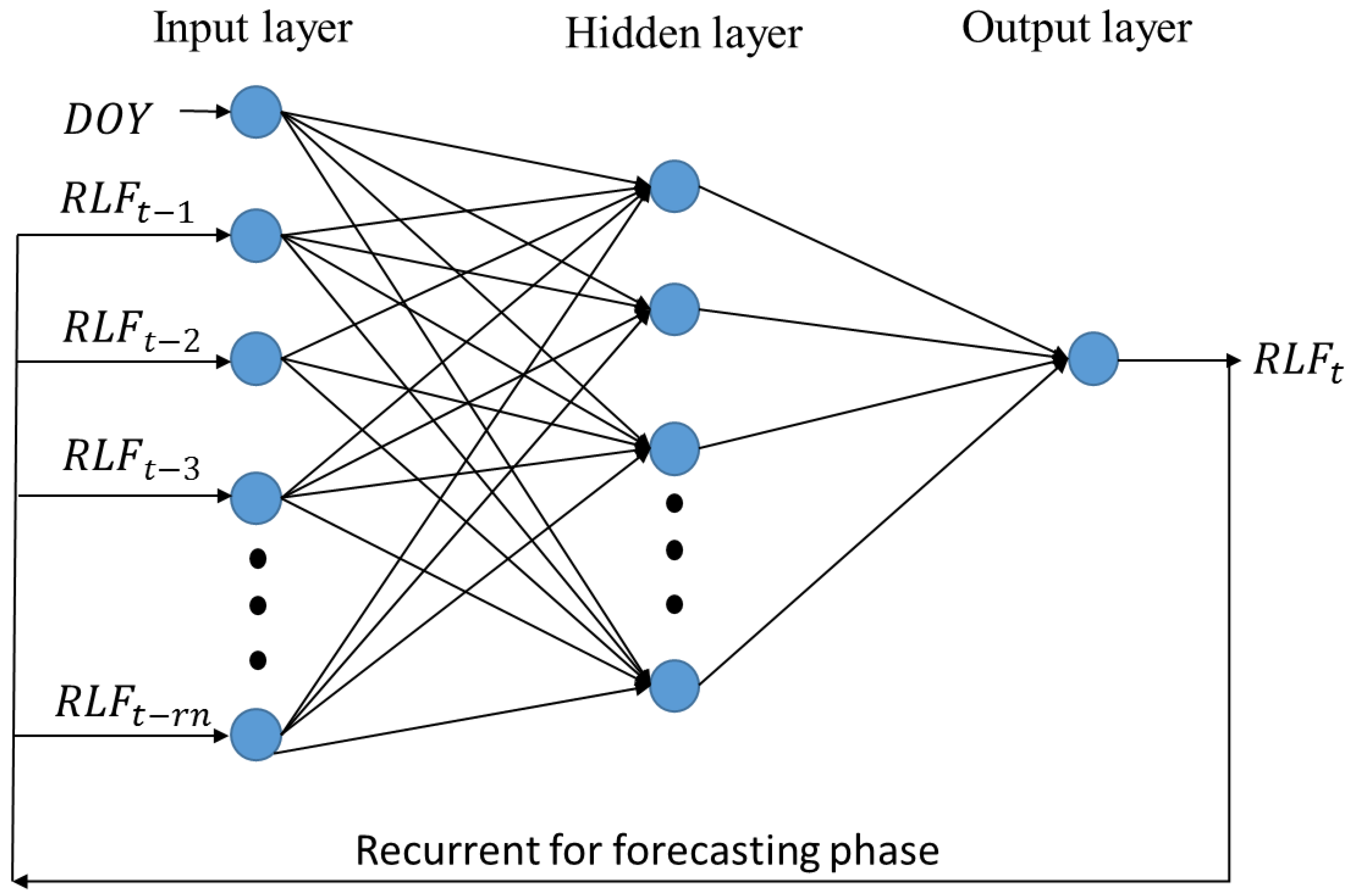
The RANN is inspired from our understanding of the human brain’s neural networks system. First, information processing is accomplished in elements which are identified as neurons; second, information is conveyed between neurons by using their connections; third, each connection has a specific weight that is a multiplier for information conveyed from one neuron to another; fourth, each neuron regularly uses a nonlinear activation function to compute its output. A RANN is described based upon network structure, training method, and activation function.
Figure 2 shows a schematic diagram of a RANN model developed in this study; RANNs are dynamic recurrent nonlinear ANNs. In RANN networks, output delays act as dynamic memory in the reservoir inflow forecasting phase. After forecasting
using RANN, the forecasted reservoir inflows by autoregressive hybrid model (
) are calculated by the following equation:
In this research, the numbers of output delays from 1 to 5 in RANN1 to RANN5 models are examined. In addition, the number of neurons in the hidden layer is tested from 1 to 30. In each test, the output of RANN ( computed by Equation (8)) and target value of the outputs ( computed by Equation (7)) are compared, and the changing of weights and bias are repeated to minimize the model error (). Then, the best RANN model is selected based on minimization of .
3. Results and Discussion
The best FSF-ARIMA model was chosen based on
and the number of parameters among multiple possible FSF-ARIMA models (
Table 1). In addition, among the examined structures, FSF-ARIMA (5, 1, 5), FSF-ARIMA (5, 1, 6), and FSF-ARIMA (1, 1, 2) had the lowest
(about 13,760). Since
values are similar in these three structures, the best model is determined based on the minimum number of parameters. The FSF-ARIMA (1, 1, 2) with the lowest
and the minimum number of parameters among FSF-ARIMA models was chosen as the best model.
The best structure among the various structures of the RANN model to forecast the daily stream flow to the Dez reservoir was selected based on minimizing
. The minimum
of training and forecasting phases for autoregressive hybrid models were 0.58 and 0.41, respectively. The selected autoregressive hybrid model uses RANN5 as its nonlinear part. RANN5 has a log sigmoid activation function,
,
,
,
,
, and
as the RANN model’s inputs, 22 neurons in the hidden layer, and one neuron in the output layer (
Table 2). The result of the best autoregressive hybrid model is selected as the proposed model and is compared with the previous FSF-ARIMA and RANN models.
Comparing the models based on evaluation indices showed that the proposed autoregressive hybrid model decreases the error of fitting in the training phase. Coefficient of determination (
) and error index (
) were used for examining the error of fitting in the training phase. The higher value of
for the proposed model indicates that the proposed model enhanced the goodness of fitting in training phase (
Table 3). In addition, the results show that the proposed autoregressive hybrid model had a smaller
than the previous FSF-ARIMA and RANN models (
Table 3). In the training phase, the
decreased by 0.44 and 0.27, and also
increased by 0.67 and 0.03 by using the proposed model compared to the FSF-ARIMA and RANN models, respectively. The comparison indicates the improvement of fitting by the proposed model in the training phase. Therefore, the results indicate significant improvement via capturing the flow pattern in the training phase by the proposed hybrid autoregressive model compared to the previous models.
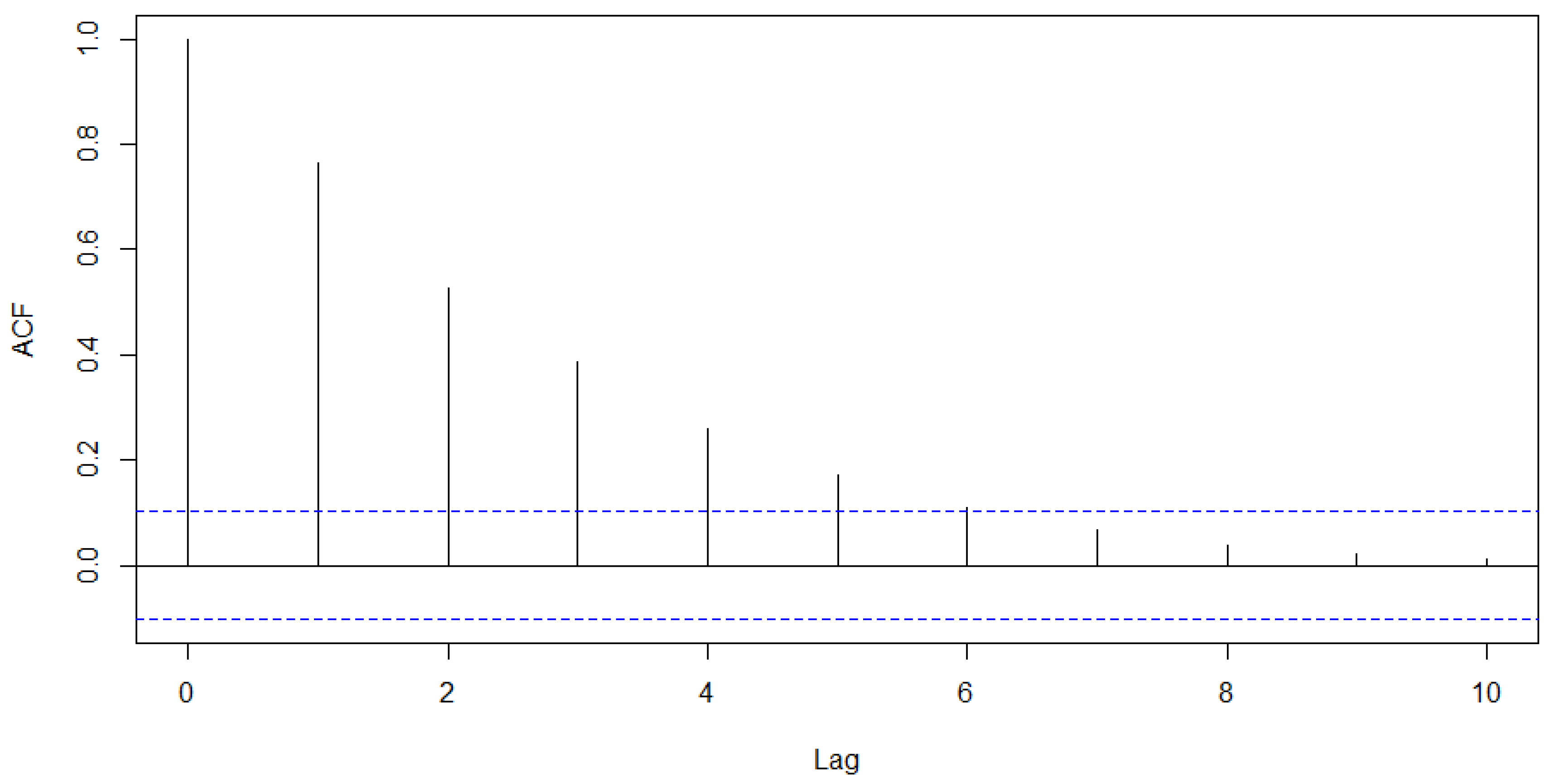
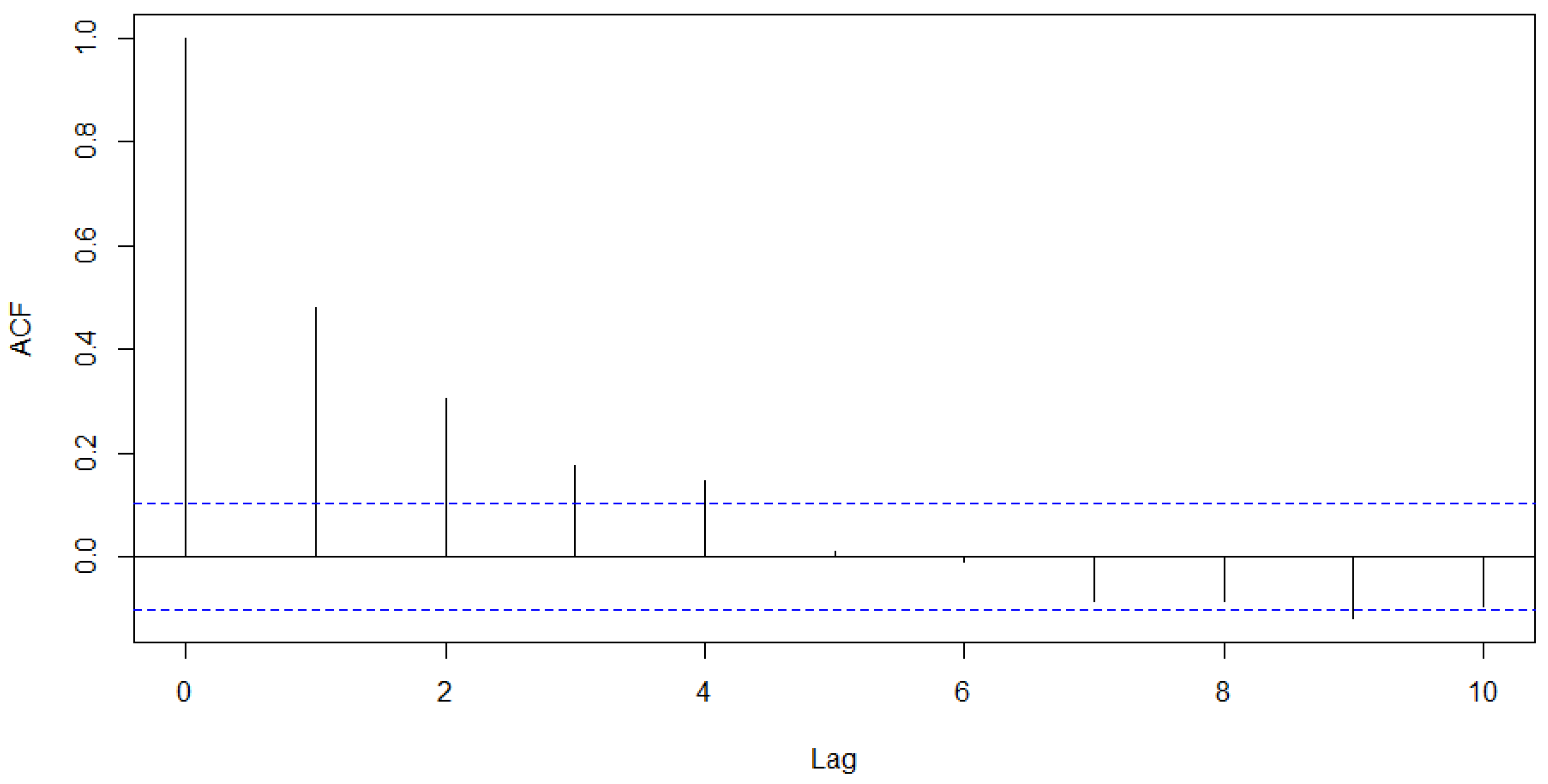
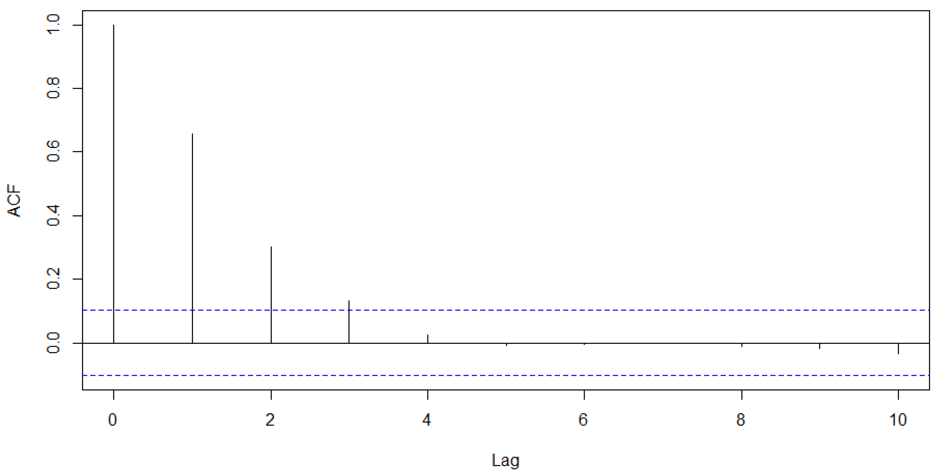
The regression evaluation metrics help to determine how close the predicted values are to the actual ones. However, they do not evaluate whether the model properly fits the data while the residuals are usually dedicated to evaluating this. Therefore, we evaluated the forecasting reliability of the proposed models by examining for auto-correlation in the errors [
35,
36].
Figure 3,
Figure 4 and
Figure 5 illustrate the autocorrelation function (ACF) diagram for Dez reservoir inflow forecasting by FSF-ARIMA model, RANN model, and Hybrid model, respectively. As we can see, most of the ACF values fall into the 95% confidence bounds, and they show a decreasing trend for increasing lag times.
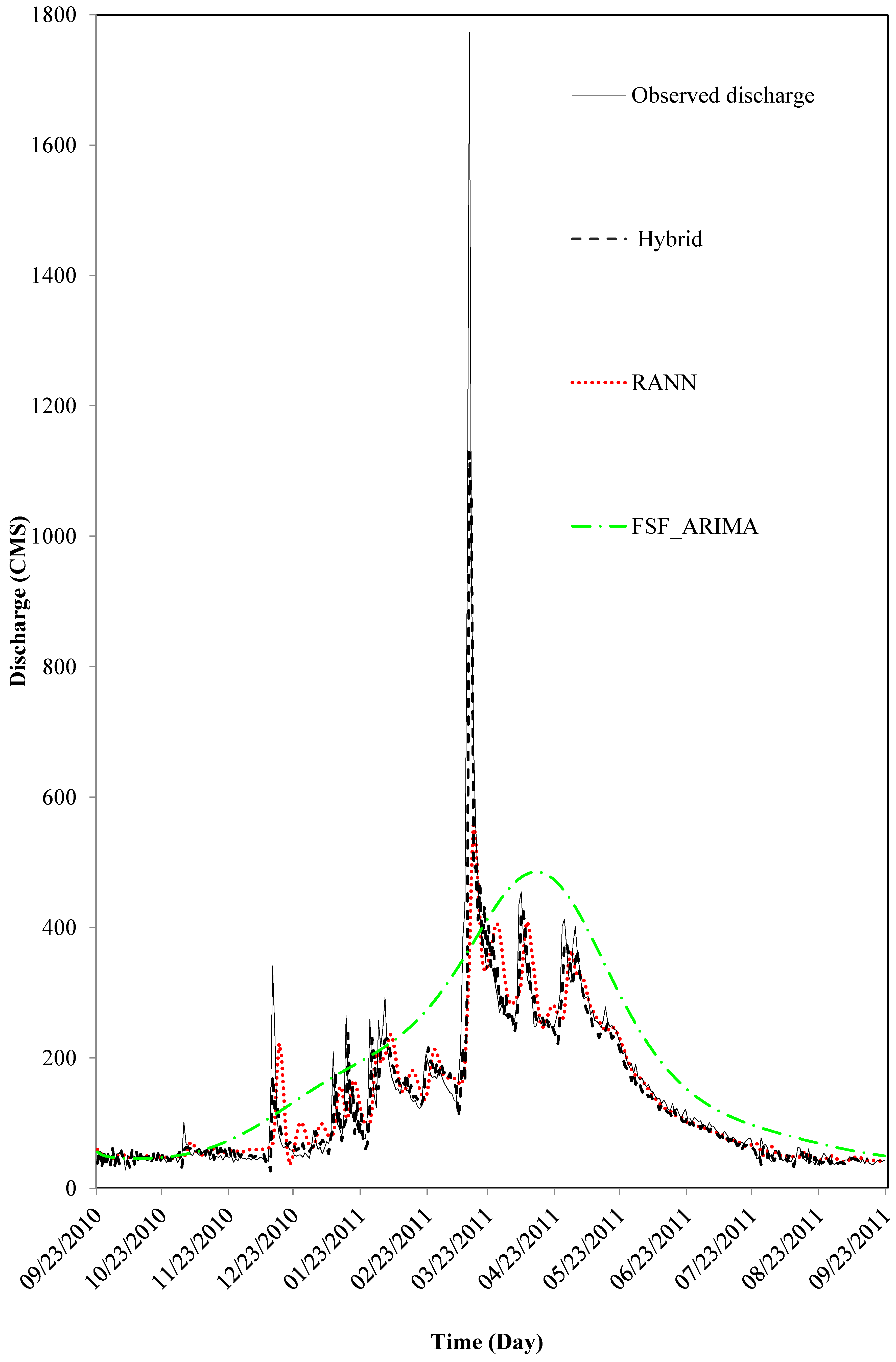
The comparison of the observed and model-based hydrographs reveals that the proposed model follows the observed flow variation better than the previous models.
Figure 6 shows the comparison of forecasted hydrographs in Cubic Meter per Second (CMS) by the models versus the observed data. However, the inflow hydrograph proposed by the RANN model follows the observed hydrograph better than that of the FSF-ARIMA model but with considerable error in forecasting peak flows (
Figure 6). Moreover,
Figure 6 displays the capability of the proposed model in following the peaks and low points of observed hydrograph. The hybrid model forecasts peak flows better than the RANN model. The proposed hybrid model forecasts the inflow values of the hydrograph precisely, whereas the FSF-ARIMA model overestimates the inflow except for the maximum peak flow (
Figure 6). In addition, the proposed autoregressive hybrid model forecasts the maximum peak flow considerably better than the RANN model by reducing the relative error from 361% to 57% compared to the previous study [
9].
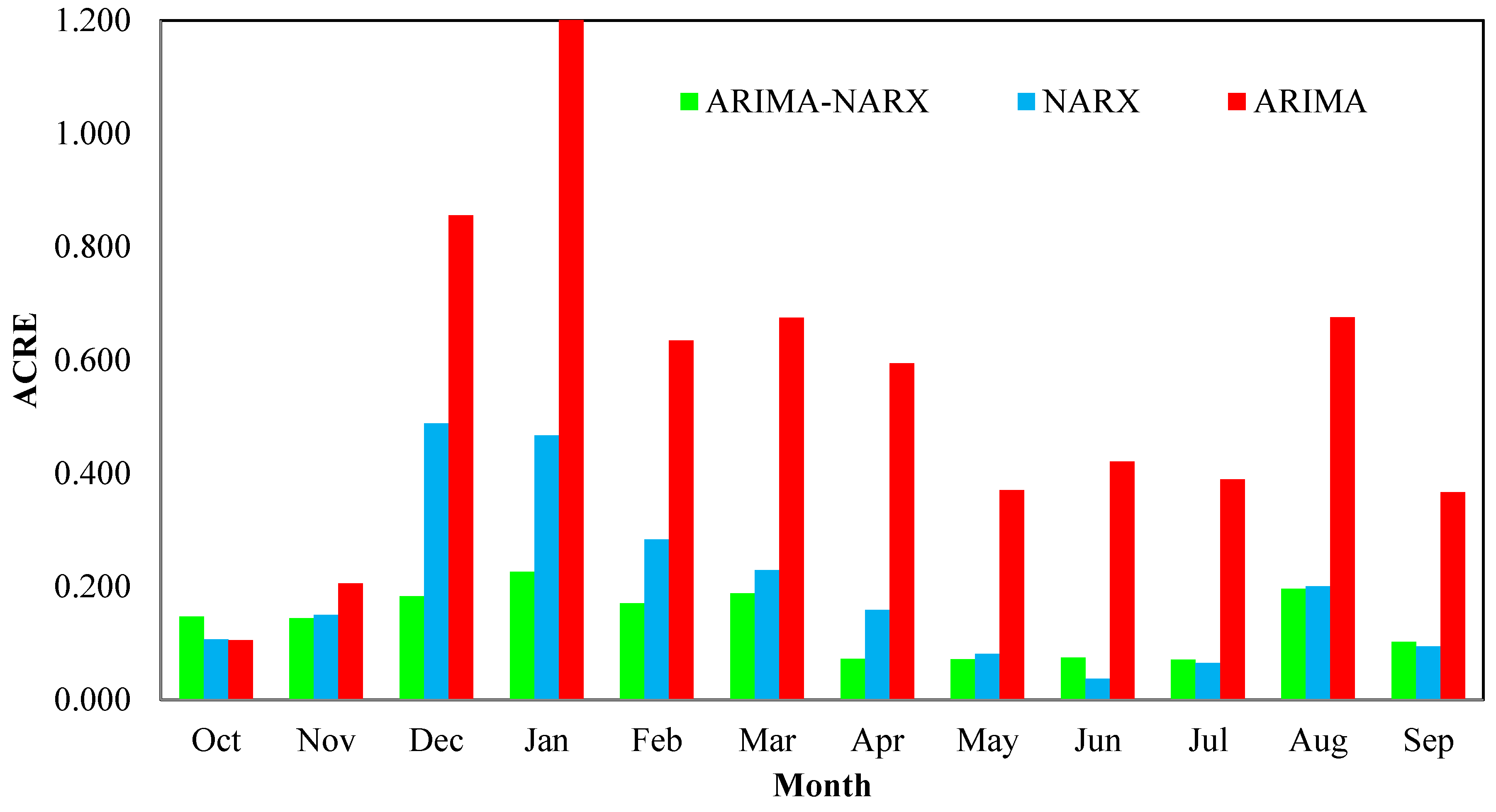
The evaluation of the models based on the
indicates that the monthly forecasting-performance of the proposed model is better than the previous models (
Figure 7). In most of the months,
for the autoregressive hybrid model is less than for the previous models. Most of the months show
higher than 0.4 for the FSF-ARIMA model. However, the proposed model decreases ACRE to less than 0.15. In addition, the maximum of
for the proposed model is considerably less than the previous models. Furthermore, the maximum and average of
for the FSF-ARIMA model are 1.2 and 0.7 for the peak season (from January to May), respectively. Those values are 0.225 and 0.15 for the proposed model. Indeed, the hybrid model has a potential to decrease maximum and average forecasting error by 81% and 80%, respectively.
4. Conclusions
In this study, an autoregressive hybrid model developed to forecast long-horizon daily inflow for optimal operation of multi-purpose reservoir with flood control, hydropower generation, domestic water supply, and irrigation goals. The proposed hybrid model comprises two parts: FSF-ARIMA (for linear part) and RANN model (nonlinear part). Since FSF-ARIMA models cannot calculate nonlinear structures of the datasets, the residuals of the FSF-ARIMA model are the nonlinear part of the stream flow time series and can be forecasted by the nonlinear part of the proposed hybrid model (RANN). The best RANN developed in this study had the log sigmoid activation function, five recurrent , , , , , 22 neurons in the hidden layer, and one neuron in the output layer. The best autoregressive hybrid model is selected as the proposed model and compared with the previous linear and nonlinear auto-regressive models (FSF-ARIMA and RANN). Comparison of the proposed autoregressive hybrid model and the previous models showed that the forecasting of long-term daily flow was significantly enhanced by the proposed hybrid model as follows:
The results demonstrated significant improvement in capturing the inflow pattern by the proposed autoregressive hybrid model from the previous models.
The monthly variations of the forecasting accuracy were extensively improved by the proposed model throughout the year and during peak season.
The proposed autoregressive hybrid model forecasted the peak flows more precisely than the previous models.
Finally, the achievement of this research compared to the current forecasting models [
9] is proposing an autoregressive hybrid model which improves the ability for forecasting reservoir inflow especially for peak flows which occurred during a one-year horizon. In [
9], NARX-RNN and ARIMA models were employed. The results of ARIMA showed
EI values equal to 0.87 and 0.85 for the training and forecasting period, respectively. Moreover, the results of NARX-RNN showed
EI values equal to 0.62 and 0.68 for training and forecasting period, respectively. Therefore, compared to
Table 3, the hybrid model developed in the current study outperforms both ARIMA and NARX-RNN which were presented by [
9]. The findings of this study can be used for optimum allocation of water resources and releasing reservoir water for optimal operation of multi-purpose reservoirs, especially in operating dams for flood control and generating hydropower. Although the hybrid model outperformed the RANN and FSF-ARIMA models, the ACF plots revealed that all models were unable to make reliable forecasts. It is worth mentioning that employing a more advanced model such as long short-term memory (LSTM) and deep learning techniques like the Convolutional Neural Network (CNN), as well as their combination, CNN-LSTM [
35,
36], can improve the accuracy of forecasting. In addition, these new models have shown more reliable forecasts [
35,
36]. Therefore, there are open avenues to compare the results of this study with LSTM and CNN-LSTM in future investigations.


