
Meta Learning for Few-Shot One-Class Classification

Department of Computer Science, Federal University of Bahia (UFBA), Salvador 40110-909, Brazil
*
Author to whom correspondence should be addressed.
†
Current address: Institute for Artificial Intelligence (AI + X), University of South Florida, Tampa, FL 33620, USA.
AI 2021, 2(2), 195-208; https://0-doi-org.brum.beds.ac.uk/10.3390/ai2020012
Submission received: 3 March 2021
/
Revised: 14 April 2021
/
Accepted: 16 April 2021
/
Published: 22 April 2021
(This article belongs to the Section AI Systems: Theory and Applications)
Abstract
:We propose a method that can perform one-class classification given only a small number of examples from the target class and none from the others. We formulate the learning of meaningful features for one-class classification as a meta-learning problem in which the meta-training stage repeatedly simulates one-class classification, using the classification loss of the chosen algorithm to learn a feature representation. To learn these representations, we require only multiclass data from similar tasks. We show how the Support Vector Data Description method can be used with our method, and also propose a simpler variant based on Prototypical Networks that obtains comparable performance, indicating that learning feature representations directly from data may be more important than which one-class algorithm we choose. We validate our approach by adapting few-shot classification datasets to the few-shot one-class classification scenario, obtaining similar results to the state-of-the-art of traditional one-class classification, and that improves upon that of one-class classification baselines employed in the few-shot setting.
1. Introduction
One-class classification algorithms, i.e., classification algorithms that learn from data from a single class and must classify unseen data as either in class or not [1], are the main approach to detecting anomalies from normal data but traditional methods scale poorly both in computational resources and sample efficiency with the data dimensions [2]. Attempting to overcome these problems, previous work proposed using deep neural networks to learn feature representations for one-class classification. While successful in addressing some of the problems, they introduced other limitations. One problem with these methods is that some of them optimize a metric that is related, but different than their true one-class classification objective (e.g., input reconstruction [3]). Other methods require imposing specific structure to the models, like using generative adversarial networks (GANs) [4,5], or removing biases and restricting the activation functions for the network model [2]. GANs are notoriously hard to optimize [6,7], and removing biases restrict which functions the models can learn [2]. Furthermore, these methods require thousands of samples from the target class, only to obtain results that are comparable to that of the traditional baselines [2].
We propose a method that overcomes these problems if we have access to data from related tasks, a notion that is better defined in Section 2.1. By using recent insights from the meta-learning community on how to learn to learn from related tasks [8,9], we show that it is possible to learn feature representations suitable for one-class classification by optimizing an estimator of its classification performance. This not only allows us to optimize the one-class classification objective without any restriction to the model besides differentiability but also improves the data efficiency of the underlying algorithm. Our method obtains similar performance to traditional methods while using 1000 times fewer data from the target class, defining a trade-off in the availability of data from related tasks and data from the target class.
For some one-class classification tasks, there are related tasks according to the definition in Section 2.1, and so our method’s requirement is satisfied. For example, in fraud detection, we could use normal activity from other users and create related tasks that consist of identifying if the activity came from the user or not, while still employing and optimizing one-class classification. Therefore, our methods and future improvements of it could be helpful in such scenarios, where user-specific data is not assumed to be available. As it is also few-shot, it could help in settings where this data is not numerous.
We describe an instance of our method, the Meta Support Vector Data Description, obtained by using the Support Vector Data Description (SVDD) [10] as the one-class classification algorithm. We also simplify this method to obtain a one-class classification variant of Prototypical Networks [9], which we call One-Class Prototypical Network. Despite its simplicity, this method obtains comparable performance to Meta SVDD. Our contributions thus are:
- We show how to learn a feature representation for one-class classification (Section 2) by defining an estimator for the classification loss of such algorithms (Section 2.1). We also describe how to efficiently backpropagate through the objective when the chosen algorithm is the SVDD method, so we can parametrize the feature representation with deep neural networks (Section 2.2). The efficiency requirement to train our model serves to make it work in the few-shot setting.
- We simplify Meta SVDD by replacing how the center of its hypersphere is computed. Instead of solving a quadratic optimization problem to find the weight of each example in the center’s averaging, we remove the weighting and make the center the result of an unweighted average (Section 3). The resulting One-Class Prototypical Networks are simpler, and have lower computational complexity and more stable training dynamics than Meta SVDD.
- After that, we detail how our method conceptually addresses the limitations of previous work (Section 4). We also show that our method has promising empirical performance by adapting two few-shot classification datasets to the one-class classification setting and obtaining comparable results with the state-of-the-art of the many-shot setting (Section 5). Our results indicate that learning the feature representations may compensate for the simplicity of replacing SVDD with feature averaging and that our approach is a viable way to replace data from the target class with labeled data from related tasks. Code to reproduce our experiments and methods is also made publicly.
Our paper is organized as follows: Section 2 briefly reviews the SVDD method and shows how we can use it for meta-learning, thus obtaining Meta SVDD; Section 3 shows that simplifying the method, we obtain a variant of the Prototypical Networks method for one-class classification; Section 4 reviews related work; Section 5 details our experiments and the observed results; and Section 6 discusses the method and future work.
2. Meta SVDD
The Support Vector Data Description (SVDD) method [10] computes the hypersphere of minimum volume that contains every point in the training set. The idea is that only points inside the hypersphere belong to the target class, so we minimize the sphere’s volume to reduce the chance of including points that do not belong in the target class.
Formally, the radius of the hypersphere centered at covering the training set X transformed by is
The SVDD objective is to find the center that minimizes the radius of such a hypersphere, i.e.,
Finally, the algorithm determines that a point belongs to the target class if
The SVDD objective, however, does not specify how to optimize the feature representation . Previous approaches include using dimensionality reduction with Principal Component Analysis (PCA) [2], using a Gaussian kernel with the kernel trick [10], or using features learned with unsupervised learning methods, like deep belief networks [11]. We take a different approach: Our goal is to learn for the task, and we detail how next.
2.1. Meta-Learning One-Class Classification
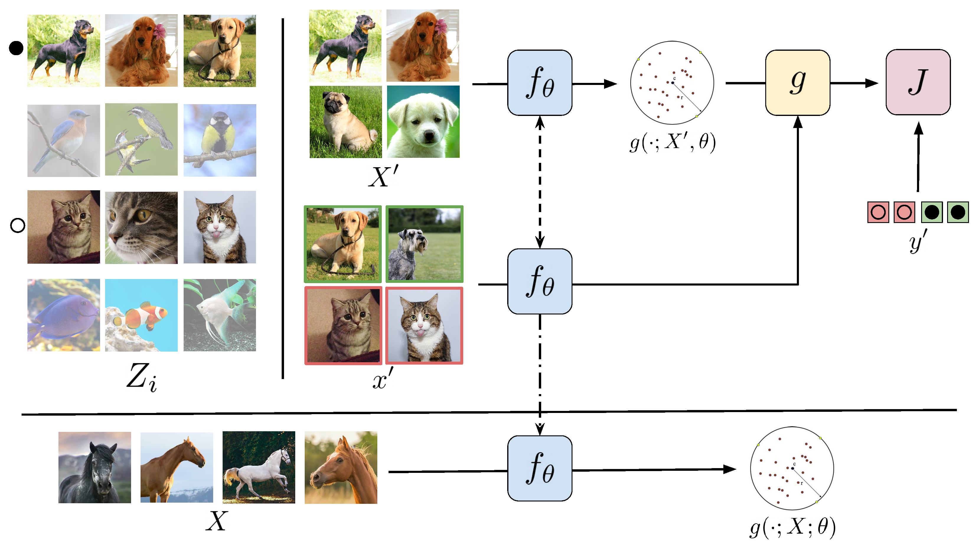
Our objective is to learn an such that the minimum volume hypersphere computed by the SVDD covers only the samples from the target class. We, therefore, divide the learning problem into two stages. In the meta-training stage, we learn the feature representation . Once we learn , we use it to learn a one-class classifier using the chosen algorithm (in this case, SVDD) from the data of the target class in the training stage. This is illustrated in Figure 1.
Notice how both the decision on unseen inputs (Equation (3)) and the hypersphere’s center (Equation (2)) depend on . Perfectly learning in the meta-training stage would map any input distribution into a space that can be correctly classified by SVDD, and would therefore not depend on the given data X nor on what is the target class; that would be learned by the SVDD after transforming X with in the subsequent training stage. We do not know how to learn perfectly but the above observation illustrates that we do not need to learn it with data from the target class.
With that observation, we can use the framework of nested learning loops [12] to describe how we propose to learn :
- Inner loop: Use to transform the inputs, and use SVDD to learn a one-class classification boundary for the resulting features.
- Outer loop: Learn from the classification loss obtained with the SVDD.
We use the expected classification loss in the outer loop. With this, we can use data that comes from the same distribution as the data for the target class, but with different classification tasks. To make this definition formal, first, let g be a one-class classification function parametrized by which receives as inputs a subset of examples from the target class and an example , and outputs the probability that belongs to the target class. For a suitable classification loss J, our learning loss is
where is a binary label indicating whether belongs to the same distribution of or not. The outer expectation of Equation (4) defines a one-class classification task, and the inner expectation is over labeled examples for this task (hence the dependency on for the labeled example distribution ). Since we do not have access to the distribution nor we have access to , we approximate it with related tasks. Intuitively, the closer the distribution of the tasks we use to approximate it, the better our feature representation.
To compute this approximation in practice, we require access to a labeled multiclass classification dataset , where is the ith element and its label, that has a distribution similar to our dataset X, but is disjoint from it (i.e., none of the elements in X are in Z and none of its elements belong to any of the classes in Z). Datasets like Z are common in the meta-learning or few-shot learning literature, and their existence is a standard assumption in previous work [8,9,13]. However, this restricts the tasks to which our method can be applied to those that have such related data available.
We then create the datasets from Z by separating its elements by class, i.e.,
We create the required binary classification tasks by picking as the data for the target class, and the examples from , , to be the input data from the negative class. Finally, we approximate the expectations in Equation (4) by first sampling mini-batches of these binary classification tasks and then averaging over mini-batches of labeled examples from each of the sampled tasks. By making each sampled have few examples (e.g., 5 or 20), we not only make our method scalable but we also learn for few-shot one-class classification.
In the next section, we define a model for and show how to optimize it over Equation (4).
2.2. Gradient-Based Optimization
If we choose to be a neural network, it is possible to optimize it to minimize the loss in Equation (4) with gradient descent as long as J and g are differentiable and have meaningful gradients because of the chain rule of calculus. J can be the standard binary cross-entropy between the data and model distributions [14].
We also modify the SVDD to satisfy the requirements of the g function. Neither how it computes the hypersphere’s center, by solving an optimization problem (Equation (2)), nor its hard, binary decisions (Equation (3)) are immediately suitable for gradient-based optimization.
To solve the hard, binary decisions problem, we adopt the approach of Prototypical Networks [9] and consider the squared distance from the features to the center (the left-hand side of Equation (3)) as the input logits for a logistic regression model. Doing this not only solves the problem of uninformative gradients coming from the binary outcomes of SVDD but also simplifies its implementation in modern automatic differentiation/machine learning software, e.g., PyTorch [15]. As our logits are non-negative, using the sigmoid function to convert logits into probabilities would result in probabilities of at least 0.5 for every input, so we replace it with the tanh and keep the binary cross-entropy objective otherwise unchanged.
As for how to compute in a differentiable manner, we can write it as the weighted average of the input features
where the weights are the solution of the following quadratic programming problem, which is the dual of the problem defined in Equation (2) [10,16]
and
is the kernel matrix of for input set X. Despite such quadratic programs not having known analytical solutions and requiring a projection operator to unroll its optimization procedure because of its inequality constraints, the quadratic programming layer [17] can efficiently backpropagate through its solution and supports GPU usage.
Still, the quadratic programming layer has complexity for m optimization variables [17]; in the case of Meta SVDD, m is equal to the number of examples in X during training [13]. As the size of the network is constant, this is the overall complexity of performing a training step in the model. Since we keep the number of examples small, 5 to 20, the runtime is dominated by the computation of .
In practice, we follow previous work that uses quadratic programming layers [13] and we add a small stabilization value to the diagonals of the kernel matrix (Equation (10)), i.e.,
and we use in Equation (7). Not adding this stabilization term results in failure to converge in some cases.
Using the program defined by objective (7), and constraints (8) and (9) to solve SVDD also allows us to use the kernel trick to make K non-linear with regards to [10]. We believe this would not add much since using a deep neural network to represent can handle the non-linearities that map the input to the output, in theory.
SVDD [10] also introduce slack variables to account for outliers in the input set X. Since our setting is few-shot one-class classification, we do not believe these would benefit the method’s performance because we think outliers are unlikely in such small samples. We leave the analysis to confirm or refute these conjectures to future work.
3. One-Class Prototypical Networks
The only reason to solve the quadratic programming problem defined by objective (7) and constraints (8) and (9) is to obtain the weights for the features of each example in Equation (6).
We experiment with replacing the weights in Equation (6) by uniform weights . The center then becomes a simple average of the input features
and we no longer require solving the quadratic program. The remainder of the method, i.e., its training objective, how tasks are sampled, etc., remains the same. This avoids the cubic complexity in the forward pass, and the destabilization issue altogether. We call this method One-Class Prototypical Networks because the method can be cast as learning binary Prototypical Networks [9] with a binary cross-entropy objective.
Despite being a simpler method than Meta SVDD, we conjecture that learning to be a good representation for One-Class Prototypical Networks can compensate its algorithmic simplicity so that performance does not degrade.
4. Related Work
4.1. One-Class Classification
We briefly survey the main ideas related to our work in the one-class classification literature. A more detailed treatment of this subject can be found in the recent survey of Perera et al. [18].
The SVDD [10], reviewed in Section 2, is closely related to the One-Class Support Vector Machines (One-Class SVMs) [1]. Whereas the SVDD finds a hypersphere to enclose the input data, the One-Class SVM finds a maximum margin hyperplane that separates the inputs from the origin of the coordinate system. Like the SVDD, it can also be formulated as a quadratic program, solved in kernelized form, and use slack variables to account for outliers in the input data. In fact, when the chosen kernel is the commonly used Gaussian kernel, both methods are equivalent [1].
Besides their equivalence in that case, the One-Class SVM more generally suffers from the same limitations as the SVDD: it requires explicit feature engineering (i.e., it prescribes no way to formulate ), and it scales poorly both with the number of samples and the dimension of the data.
In Section 2, we propose to learn from related tasks, which addresses the feature engineering problem. We also make it so that it requires only a small set to learn the one-class classification boundary, solving the scalability problem in the number of samples. Finally, by making the feature dimension d much smaller than D, we solve the scalability issue regarding the feature dimensionality.
The limitations of SVDD and One-Class SVMs led to the development of deep approaches to one-class classification, where the previous approaches are known as shallow because they do not rely on deep (i.e., multi-layered) neural networks for feature representation.
Most previous approaches that use deep neural networks to represent the input feature for downstream use in one-class classification algorithms are trained with a surrogate objective, like the representation learned for input reconstruction with deep autoencoders [19].
Autoencoder methods learn feature representations by requiring the network to reconstruct inputs while preventing it to learn the identity function. These are usually divided into an encoder, tasked with converting an input example into an intermediate representation, and a decoder, that gets the representation and must reconstruct the input [14].
The idea is that if the identity function cannot be learned, then the representation has captured semantic information of the input that is sufficient for its partial reconstruction and other tasks. How the identity function is prevented determines the type of autoencoder and many options exist: by reducing the dimensions of or imposing specific distributions to the intermediate representations, by adding a regularization term to the model’s objective, or by corrupting the input with noise [14].
Philipp Seeböck et al. [3] train a deep convolutional autoencoder (DCAE) in images for the target class, here healthy retinal image data, and after that the decoder is ignored and a One-Class SVM is trained on the resulting intermediate representations. The main issue with this approach is that the objective of autoencoder training does not assure that the learned representations are useful for classification.
A related approach is to reuse features from networks trained for multiclass classification. Oza and Patel [20] remove the softmax layer of a Convolutional Neural Network (CNN) [21] trained in the ImageNet dataset [22] as its feature extractor. The authors then train the fully-connected layers of the pre-trained network alongside a new fully connected layer tasked with discriminating between features from the target class and data sampled from a spherical Gaussian distribution; the convolutional layers are not updated.
AnoGANs [5] are trained as Generative Adversarial Networks [4] to generate samples from the target class. After that, gradient descent is used to find the sample in the noise distribution that best reconstructs the unseen example to be classified, which is equivalent to approximately inverting the generator using optimization. The classification score is the input reconstruction error, which assumes pixel-level similarity determines membership in the target class.
Like our method, Deep SVDD [2] attempts to learn feature representations for one-class classification from the data using gradient-based optimization with a neural network model. It consists of directly reducing the volume of a hypersphere containing the features, and in that it is a deep version of the original SVDD.
Deep SVDD’s algorithm relies on setting the centers every few iterations with the mean of the features from a forward pass instead of computing the minimum bounding sphere. Since their objective is to minimize the volume of the hypersphere containing the features, the algorithm must avoid the pathological solution of outputting a constant function. This requires imposing architectural constraints on the network, the stronger of which is that the network’s layers can have no bias terms. The authors also initialize the weights with those of an encoder from a trained autoencoder. Neural network models in our method have no such restrictions and do not require a pre-training stage.
One advantage of Deep SVDD over our work is that it does not require data from tasks from a similar distribution: it is trained only on the target class data. While this is an advantage, there is a downside to it. It is not clear for us, reading the paper describing Deep SVDD, how to know for how long to train a Deep SVDD model, how to tune its many hyperparameters, or what performance to expect of the method in unseen data. These are usually done with computing useful metrics in a validation set. However, for Deep SVDD, the optimal value can be reached for pathological solutions, so a validation set is not useful.
Ruff et al. [2] prove that using certain activation functions or keeping bias terms allow the model to learn the constant function but they do not prove the reciprocate, i.e., they do not prove that constant functions cannot be learned by the restricted models. The authors also do not analyze which functions are no longer learnable when the model is restricted as such. For Meta SVDD, on the other hand, the related tasks give predictive measures of metrics of interest, allow tuning hyperparameters, and early stopping.
4.2. Few-Shot Learning
The main inspiration for the ideas in our paper besides Deep SVDD came from the field of meta-learning, in particular, that of few-shot classification. Prototypical Networks [9] are few-shot classifiers that create prototypes from few labeled examples and use their squared distances to an unseen example as the logits to classify it as one of their classes. We first saw the idea of learning the feature representation from similarly distributed tasks and of using the squared distances in this paper. They also propose feature averaging as a way to summarize class examples and show its competitive performance despite its simplicity; One-Class Prototypical Networks are the one-class variant of this method.
Recently, Lee et al. [13] proposed to learn feature representations for few-shot classification convex learners, including multi-class Support Vector Machines [23], with gradient-based optimization. Their work is similar to ours in its formulation of learners as quadratic programs, and in solving these with quadratic programming layers but it does not address one-class classification.
4.3. Few-Shot, One-Class Classification
Concurrent with our work, others have started investigating the use of few-shot classification methods for the one-class classification task. Most similar to our work, Oladosu et al. [24] propose to perform meta-learning in a setting that is similar to ours, i.e., their method is trained with multiple supervised tasks so it can perform on unseen tasks with only positive example at deploy time. The main differences between our methods is that theirs uses set equivariant networks to learn representations from the positive examples, whereas we use either SVDD or a Prototypical Network layer. Like us, they also evaluate their method by adapting datasets with supervision to the meta-learning one-class setting by splitting them over the labels instead of over examples.
5. Experiments
5.1. Evaluation Protocol
Our first experiment is an adaptation of the evaluation protocol of Deep SVDD [2] to the few-shot setting to compare Meta SVDD with previous work. The original evaluation protocol consists of picking one of the classes of the dataset, training the method in the examples in the training set (using the train-test split proposed by the maintainers), and using all the examples in the test set to compute the mean and standard deviation of the area under the curve (AUC) of the trained classifier over 10 repetitions in the MNIST [25] and CIFAR-10 [26] datasets.
We modified the protocol because there ertr only 10 classes in these datasets, which esd not enough for meta-learning one-class classifiers. This illustrates the trade-off introduced by our approach: despite requiring many fewer examples per class, it requires many more classes. Our modifications were only to address the number of classes and we tried to keep the protocol as similar as possible to make the results more comparable.
5.1.1. Datasets
The first modification was the replacement of CIFAR-10 by the CIFAR-FS dataset [27], a new split of CIFAR-100 for few-shot classification in which there was no class overlap between the training, validation and test sets. CIFAR-FS had 64 classes for training, 16 for validating, and 20 for testing, and each class had 600 images. This resulted in a split of 64% of the data for training, 16% for validation and 20% for testing in the CIFAR-FS dataset.
No such split was possible for MNIST because there was no fine-grained classification like in the case of the CIFAR-10 and CIFAR-100 datasets. Therefore, we used the Omniglot dataset [28], which is considered the “transposed” version of the MNIST dataset because it has many classes with few examples instead of the many examples in the 10 classes of MNIST. This dataset consisted of 20 images of each of its 1623 handwritten characters, which were usually augmented with four multiples of to obtain classes [8,9,27,29]. We followed the pre-processing and dataset split proposed by Vinylas et al. [29] by resizing the images to pixels, and using 4800 classes for training and 1692 for testing, which is nowadays standard in few-shot classification work [8,9,27]. Hence, we had approximately 73% of the data for training and 26% of the data for testing in the Omniglot dataset.
We also modified the number of elements per class in the test set evaluation. Since there were many classes and we were dealing with few-shot classification, we used only two times the number of examples in X for the target and for the negative class, e.g., if the task was five-shot learning, then there were 10 examples from the target class and 10 examples from the negative class for evaluation.
5.1.2. Metrics and Comparison
Another modification, since there were only 10 classes in MNIST and CIFAR-10, Deep SVDD [2] reports the AUC metrics for each class. This was feasible for CIFAR-FS, which had 20 testing classes, but not for Omniglot, which had 1692. We summarized these statistics by presenting the minimum, median, and maximum mean AUC alongside their standard deviations.
To better compare the previous methods with ours in the few-shot setting, we evaluated the state-of-the-art method for general deep one-class classification, Deep SVDD [2], in our modified protocol. We ran the evaluation protocol in CIFAR-FS using only five images for training, and we evaluated it using 10 images from the target class and 10 images from a negative class, and we did this 10 times for each pair of the 20 test classes to compute mean and standard deviation statistics for the AUC. We did not do this for Omniglot because it required training more than 1692 Deep SVDD models.
5.1.3. Second Experiment
We also conducted a second experiment, based on the standard few-shot classification experiment in which we evaluated the mean five-shot one-class classification accuracy over 10,000 episodes of tasks consisting of 10 examples from the target class and 10 examples from the negative class. We used this experiment to compare with a shallow baseline, PCA and Gaussian kernel One-Class SVM [1], and One-Class Prototypical Network. We used the increased number of episodes to compute 95% confidence intervals like previous work for few-shot multiclass classification [13,27].
5.2. Setup
5.2.1. Network Architecture
We parametrized with the neural network architecture model introduced by Vinyalset al. [29] that is commonly used in other few-shot learning work [8,9]. This convolutional neural network (CNN) had four convolutional blocks with number of filters equal to 64, and each block was composed of a kernel, stride 1, “same” 2D convolution, batch normalization [30], followed by max-pooling and ReLU activations [31].
We implemented the neural network using PyTorch [15] (version 1.2.0) and the qpth package [17] (version 0.0.15) for the quadratic programming layer. We also used Scikit-Learn [32] (version 0.21.3) and NumPy [33] (version 1.17.3) to compute metrics, implement the shallow baselines and for miscellaneous tasks, and Torchmeta [34] (version 1.1.1) to sample mini-batches of tasks, like described in Section 2.1. All our code is publicly available at https://github.com/gdahia/meta_occ/ (accessed on 3 March 2021).
5.2.2. Optimization and Hyperparameters
We optimized both Meta SVDD and One-Class Prototypical Networks using stochastic gradient descent [35] on the objective defined in Section 2.1 and Equation (4) with the Adam optimizer [36]. We used a constant learning rate of over mini-batches of tasks of size 16, each having set with five examples, and set with 10 examples from the target class and 10 examples from a randomly picked negative class. The learning rate value was the first one we tried, so no tuning was required. We picked the task batch size that performed better in the validation set when training halts; we tried sizes . We evaluated the performance in the validation set with 95% confidence intervals of the model’s accuracy in 500 tasks randomly sampled from the validation sets, and we considered that a model was better than another if the lower bound of its confidence interval was greater, or if its mean was higher when the lower bounds were equal up to five decimal points. Early stopping halted training when performance in the validation set did not increase for 10 evaluations in a row, and we used the model with higher performance in the validation set. We evaluated the model in the validation set every 100 training steps.
5.2.3. Baslines
The results for the few-shot experiment with Deep SVDD were obtained modifying the code made available by the authors (https://github.com/lukasruff/Deep-SVDD-Pytorch, accessed on 3 March 2021), keeping the same hyperparameters.
For the few-shot baseline accuracy experiment with PCA and One-Class SVMs with Gaussian kernel, we used the grid search space used by the experiments in prior work [2]: was selected from , and was selected from . Furthermore, we gave the shallow baseline an advantage by evaluating every parameter combination in the test set and reporting the best result.
5.3. Results
5.3.1. First Experiment
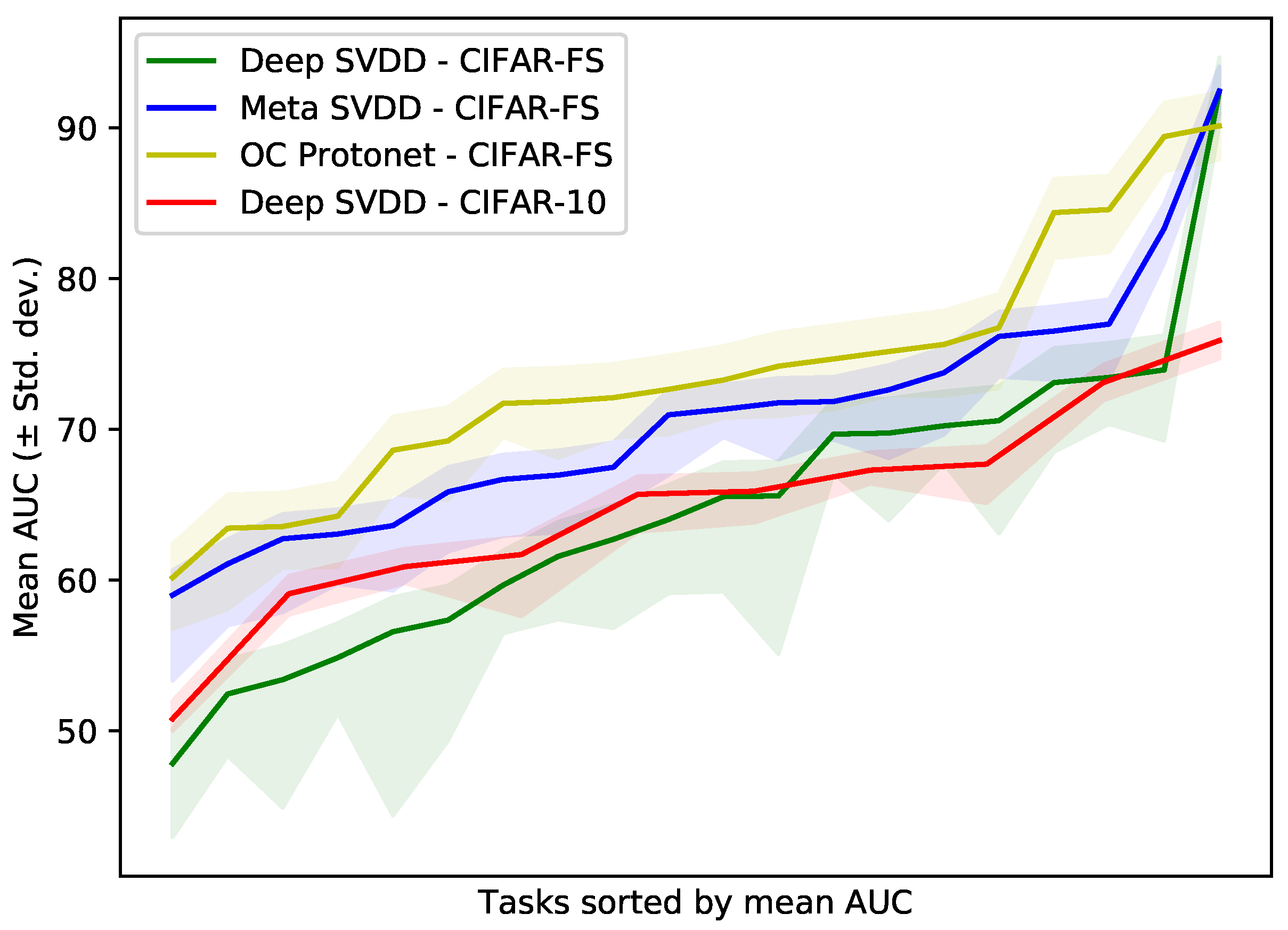
We reproduce the results reported for Deep SVDD [2] and its baselines alongside the results for five-shot Meta SVDD and One-Class Prototypical Networks, and our experiment with five-shot Deep SVDD in Table 1. Figure 2 also provides mean AUC with shaded standard deviations for the results in the CIFAR dataset variants.
While the results from different datasets were not comparable due to the differences in setting and application listed in Section 5.1, they showed that the approach had similar performance to the many-shot state-of-the-art in terms of AUC. Figure 2 shows that when we sorted the mean AUCs for CIFAR-10 and CIFAR-FS, the performance from hardest to easier tasks exhibited similar trends despite these differences, and that the modifications to the protocol were reasonable.
This experiment is evidence that our method was able to reduce the required amount of data from the target class in case we have labeled data from related tasks. Note that it was not the objective of our experiments to show that our method had better performance than previous approaches, since they operate in different settings, i.e., few-shot with related tasks and many-shot without them.
The comparison with Deep SVDD in the few-shot scenario gave further evidence of the relevance of our method: both Meta SVDD and One-Class Prototypical Networks obtain higher minimum, and median AUC than Deep SVDD. Another advantage was that we trained once in the training set of Omniglot or CIFAR-FS, and learned only either the SVDD or the average on each of the sets X in the test set. We also obtained these results without any pre-training, and we established a clear validation procedure to guide hyperparameter tuning and early stopping.
These results also showed we could train a neural network for without architectural restrictions to optimize a one-class classification objective whereas other methods either required feature engineering, optimize another metric, or imposed restrictions on the model architecture to prevent learning trivial functions.
5.3.2. Second Experiment
The results for our second experiment, comparing the accuracies of Meta SVDD, a shallow baseline and One-Class Prototypical Networks, are presented in Table 2.
In this experiment, we could see an increase from almost random performance to almost perfect performance for both methods when compared to the shallow baseline in Omniglot. Both methods for few-shot one-class classification that used related tasks had equivalent performance in Omniglot. The gain was not as significant for CIFAR-FS but more than 10% in absolute for both methods, which showed they were a marked improvement over the shallow baseline.
Comparing the two proposed methods, we observed the unexpected result that the simpler method, One-Class Prototypical Networks, had equivalent accuracy in the Omniglot experiment, and better accuracy in the CIFAR-FS experiment. This indicated that learning the feature representation directly from data might be more important than the one-class classification algorithm we chose, and the increased complexity of using SVDD over simple averaging did not translate into improved performance in this setting.
5.3.3. Other Experiments
We also attempted to run this same experiment with the miniImageNet dataset [29], a dataset for few-shot learning using the images from the ImageNet dataset [22]. The accuracy in the validation set, however, never rose above 50%. One of the motivations of introducing CIFAR-FS was that there was a gap in the challenge between training models in Omniglot and miniImageNet and that successfully training models in the latter took hours [27]. Since none of the previous methods attempted solving ImageNet level datasets, and the worst performance in datasets from CIFAR is already near random guessing, we leave the problem of training one-class classification algorithms in this dataset open for future work.
Finally, we ran a small variation of the second experiment in which the number of examples in X is greater than during training, using 10 examples instead of five. The results stayed within the accuracy confidence intervals for five-shot for both models in this 10-shot deployment scenario.
6. Conclusions
We have described a way to learn feature representations so one-class classification algorithms can learn decision boundaries that contain the target class from data, optimizing an estimator of its true objective. Furthermore, this method works with five samples from the target class with performance similar to the state-of-the-art in the setting where target class data is abundant, and better when the many-shot state-of-the-art method is employed in the few-shot setting. We also provide an experiment that shows that using a simpler one-class classification yields comparable performance, displaying the advantages of learning feature representations directly from data.
One possibility to replace the main requirement of our method with a less limiting one would be the capability of generating related tasks from unlabeled data. A simple approach in this direction could be using weaker learners to define pseudolabels for the data. Doing this successfully would increase the number of settings where our method can be used significantly.
The main limitations of our method besides the requirement of the related tasks are the destabilization of the quadratic programming layer, which we solved by adding a stabilization term to the diagonal of the kernel matrix or by simplifying the one-class classification algorithm to use the mean of the features, and its failure to obtain meaningful results in the miniImageNet dataset.
We believe not only finding solutions to these limitations should be investigated in future work but also other questions left open in our work, like confirming our hypothesis that introducing slacks would not benefit Meta SVDD.
Other directions for future work are extending our method for other settings and using other one-class classification methods besides SVDD. Tax and Duin [10] also detail a way to incorporate negative examples in the SVDD objective, so we could try learning using this method and to minimize the hypersphere’s volume instead of converting SVDD into a binary classification problem that uses the unseen examples’ distances to the center as logits.
Author Contributions
All authors (G.D. and M.P.S.) contributed equally to this work. All authors have read and agreed to the published version of the manuscript.
Funding
This research received no external funding.
Data Availability Statement
Publicly available datasets were analyzed in this study. This data can be found here: https://github.com/gdahia/meta_occ, https://github.com/brendenlake/omniglot, http://www.cs.toronto.edu/~kriz/cifar.html.
Conflicts of Interest
The authors declare no conflict of interest.
References
- Schölkopf, B.; Platt, J.C.; Shawe-Taylor, J.; Smola, A.J.; Williamson, R.C. Estimating the Support of a High-Dimensional Distribution. Neural Comput. 2001, 13, 1443–1471. [Google Scholar] [CrossRef] [PubMed]
- Ruff, L.; Vandermeulen, R.; Goernitz, N.; Deecke, L.; Siddiqui, S.A.; Binder, A.; Müller, E.; Kloft, M. Deep One-Class Classification. In Proceedings of the 35th International Conference on Machine Learning, Stockholm, Sweden, 10–15 July 2018; Dy, J., Krause, A., Eds.; PMLR: Stockholm, Sweden, 2018; Volume 80, pp. 4393–4402. [Google Scholar]
- Seeböck, P.; Waldstein, S.M.; Klimscha, S.; Gerendas, B.S.; Donner, R.; Schlegl, T.; Schmidt-Erfurth, U.; Langs, G. Identifying and Categorizing Anomalies in Retinal Imaging Data. arXiv 2016, arXiv:1612.00686. [Google Scholar]
- Goodfellow, I.J.; Pouget-Abadie, J.; Mirza, M.; Xu, B.; Warde-Farley, D.; Ozair, S.; Courville, A.C.; Bengio, Y. Generative Adversarial Nets. In Proceedings of the Advances in Neural Information Processing Systems 27: Annual Conference on Neural Information Processing Systems 2014, Montreal, QC, Canada, 8–13 December 2014; pp. 2672–2680. [Google Scholar]
- Schlegl, T.; Seeböck, P.; Waldstein, S.M.; Schmidt-Erfurth, U.; Langs, G. Unsupervised Anomaly Detection with Generative Adversarial Networks to Guide Marker Discovery. In Proceedings of the Information Processing in Medical Imaging—25th International Conference (IPMI 2017), Boone, NC, USA, 25–30 June 2017; pp. 146–157. [Google Scholar] [CrossRef] [Green Version]
- Arjovsky, M.; Chintala, S.; Bottou, L. Wasserstein GAN. arXiv 2017, arXiv:1701.07875. [Google Scholar]
- Mescheder, L.; Geiger, A.; Nowozin, S. Which Training Methods for GANs do actually Converge? In Proceedings of the 35th International Conference on Machine Learning, Stockholm, Sweden, 10–15 July 2018; Dy, J., Krause, A., Eds.; PMLR: Stockholm, Sweden, 2018; Volume 80, pp. 3481–3490. [Google Scholar]
- Finn, C.; Abbeel, P.; Levine, S. Model-Agnostic Meta-Learning for Fast Adaptation of Deep Networks. In Proceedings of the 34th International Conference on Machine Learning (ICML’17), Sydney, Australia, 6–11 August 2017; Volume 70, pp. 1126–1135. [Google Scholar]
- Snell, J.; Swersky, K.; Zemel, R.S. Prototypical Networks for Few-shot Learning. In Proceedings of the Advances in Neural Information Processing Systems 30: Annual Conference on Neural Information Processing Systems 2017, Long Beach, CA, USA, 4–9 December 2017; pp. 4077–4087. [Google Scholar]
- Tax, D.M.J.; Duin, R.P.W. Support Vector Data Description. Mach. Learn. 2004, 54, 45–66. [Google Scholar] [CrossRef] [Green Version]
- Erfani, S.M.; Rajasegarar, S.; Karunasekera, S.; Leckie, C. High-dimensional and large-scale anomaly detection using a linear one-class SVM with deep learning. Pattern Recognit. 2016, 58, 121–134. [Google Scholar] [CrossRef]
- Raghu, A.; Raghu, M.; Bengio, S.; Vinyals, O. Rapid Learning or Feature Reuse? Towards Understanding the Effectiveness of MAML. arXiv 2019, arXiv:1909.09157. [Google Scholar]
- Lee, K.; Maji, S.; Ravichandran, A.; Soatto, S. Meta-Learning with Differentiable Convex Optimization. In Proceedings of the IEEE Conference on Computer Vision and Pattern Recognition (CVPR), Long Beach, CA, USA, 15–20 June 2019. [Google Scholar]
- Goodfellow, I.; Bengio, Y.; Courville, A. Deep Learning; MIT Press: Cambridge, MA, USA, 2016; Available online: http://www.deeplearningbook.org (accessed on 3 March 2021).
- Paszke, A.; Gross, S.; Massa, F.; Lerer, A.; Bradbury, J.; Chanan, G.; Killeen, T.; Lin, Z.; Gimelshein, N.; Antiga, L.; et al. PyTorch: An Imperative Style, High-Performance Deep Learning Library. In Advances in Neural Information Processing Systems 32; Curran Associates, Inc.: Nice, France, 2019; pp. 8024–8035. [Google Scholar]
- Elzinga, D.J.; Hearn, D.W. The minimum covering sphere problem. Manag. Sci. 1972, 19, 96–104. [Google Scholar] [CrossRef]
- Amos, B.; Kolter, J.Z. OptNet: Differentiable Optimization as a Layer in Neural Networks. In Proceedings of the 34th International Conference on Machine Learning, Sydney, Australia, 6–11 August 2017; Precup, D., Teh, Y.W., Eds.; International Convention Center: Sydney, Australia, 2017; Volume 70, pp. 136–145. [Google Scholar]
- Perera, P.; Oza, P.; Patel, V.M. One-Class Classification: A Survey. arXiv 2021, arXiv:2101.03064. [Google Scholar]
- Hinton, G.E.; Salakhutdinov, R.R. Reducing the Dimensionality of Data with Neural Networks. Science 2006, 313, 504–507. [Google Scholar] [CrossRef] [PubMed] [Green Version]
- Oza, P.; Patel, V.M. One-Class Convolutional Neural Network. IEEE Signal Process. Lett. 2019, 26, 277–281. [Google Scholar] [CrossRef] [Green Version]
- LeCun, Y.; Boser, B.E.; Denker, J.S.; Henderson, D.; Howard, R.E.; Hubbard, W.E.; Jackel, L.D. Handwritten digit recognition with a back-propagation network. In Proceedings of the Advances in Neural Information Processing Systems, Denver, CO, USA, 26–29 November 1990; pp. 396–404. [Google Scholar]
- Deng, J.; Dong, W.; Socher, R.; Li, L.; Li, K.; Li, F. ImageNet: A large-scale hierarchical image database. In Proceedings of the 2009 IEEE Computer Society Conference on Computer Vision and Pattern Recognition (CVPR 2009), Miami, FL, USA, 20–25 June 2009; pp. 248–255. [Google Scholar] [CrossRef] [Green Version]
- Cortes, C.; Vapnik, V. Support-Vector Networks. Mach. Learn. 1995, 20, 273–297. [Google Scholar] [CrossRef]
- Oladosu, A.; Xu, T.; Ekfeldt, P.; Kelly, B.A.; Cranmer, M.; Ho, S.; Price-Whelan, A.M.; Contardo, G. Meta-Learning for Anomaly Classification with Set Equivariant Networks: Application in the Milky Way. arXiv 2020, arXiv:2007.04459. [Google Scholar]
- LeCun, Y.; Bottou, L.; Bengio, Y.; Haffner, P. Gradient-based learning applied to document recognition. Proc. IEEE 1998, 86, 2278–2324. [Google Scholar] [CrossRef] [Green Version]
- Krizhevsky, A. Learning Multiple Layers of Features from Tiny Images. Technical Report. 2009. Available online: http://www.cs.toronto.edu/~kriz/learning-features-2009-TR.pdf (accessed on 21 April 2021).
- Bertinetto, L.; Henriques, J.F.; Torr, P.H.S.; Vedaldi, A. Meta-learning with differentiable closed-form solvers. In Proceedings of the 7th International Conference on Learning Representations (ICLR 2019), New Orleans, LA, USA, 6–9 May 2019. [Google Scholar]
- Lake, B.M.; Salakhutdinov, R.; Tenenbaum, J.B. Human-level concept learning through probabilistic program induction. Science 2015, 350, 1332–1338. [Google Scholar] [CrossRef] [Green Version]
- Vinyals, O.; Blundell, C.; Lillicrap, T.; Kavukcuoglu, K.; Wierstra, D. Matching Networks for One Shot Learning. In Proceedings of the Advances in Neural Information Processing Systems 29: Annual Conference on Neural Information Processing Systems 2016, Barcelona, Spain, 5–10 December 2016; pp. 3630–3638. [Google Scholar]
- Ioffe, S.; Szegedy, C. Batch Normalization: Accelerating Deep Network Training by Reducing Internal Covariate Shift. In Proceedings of the 32nd International Conference on Machine Learning (ICML 2015), Lille, France, 6–11 July 2015; pp. 448–456. [Google Scholar]
- Jarrett, K.; Kavukcuoglu, K.; Ranzato, M.; LeCun, Y. What is the best multi-stage architecture for object recognition? In Proceedings of the IEEE 12th International Conference on Computer Vision (ICCV 2009), Kyoto, Japan, 27 September–4 October 2009; pp. 2146–2153. [Google Scholar] [CrossRef] [Green Version]
- Pedregosa, F.; Varoquaux, G.; Gramfort, A.; Michel, V.; Thirion, B.; Grisel, O.; Blondel, M.; Prettenhofer, P.; Weiss, R.; Dubourg, V.; et al. Scikit-learn: Machine Learning in Python. J. Mach. Learn. Res. 2011, 12, 2825–2830. [Google Scholar]
- Oliphant, T. NumPy: A guide to NumPy; Trelgol Publishing: Spanish Fork, UT, USA, 2006. [Google Scholar]
- Deleu, T.; Würfl, T.; Samiei, M.; Cohen, J.P.; Bengio, Y. Torchmeta: A Meta-Learning Library for PyTorch. 2019. Available online: https://github.com/tristandeleu/pytorch-meta (accessed on 3 March 2021).
- Robbins, H.; Monro, S. A Stochastic Approximation Method. Ann. Math. Stat. 1951, 22, 400–407. [Google Scholar] [CrossRef]
- Kingma, D.P.; Ba, J. Adam: A Method for Stochastic Optimization. In Proceedings of the 3rd International Conference on Learning Representations, Conference Track Proceedings (ICLR 2015), San Diego, CA, USA, 7–9 May 2015. [Google Scholar]
Figure 1.
Overview of the proposed method. During the meta-training stage, we emulate a training stage by first sampling from a distribution that is similar to the one of our target class data X. In practice we use all examples from class i—represented as the sets in the figure—from a labeled dataset Z. We then sample a minibatch of pairs with being an example and a binary label indicating whether belongs to the same class as the examples in , sampling again from sets . Then, we use a one-class classification algorithm (e.g., SVDD) in the features resulting from applying on the examples of . We use the resulting classifier to classify each example’s features as belonging or not to the same class as , and compute the binary loss J with the true labels . We optimize by doing gradient descent in the value of J over many such tasks. After is learned, we run the same one-class classification algorithm on the resulting features, represented by the dashed-dotted arrow from the meta-training to the deployment stage, for X in the true training stage, yielding the final one-class classification method.

Figure 2.
Mean AUC with shaded standard deviations for tasks in CIFAR datasets sorted by increasing mean value. Comparing Deep SVDD across datasets and protocols shows that the modified protocol is reasonable to evaluate few-shot one-class classification because the trend in task difficulty is similar. Within the few-shot protocol in CIFAR-FS, meta one-class classification are numerically superior, show less variance and can be meta-trained once for all tasks, with simple adaptation for unseen tasks, but require related task data.


Table 1.
Minimum, median and maximum mean AUC alongside their standard deviation for one-class classification methods for 10 repetitions. We highlight in boldface the highest mean and others which are within one standard deviation from it. The results for the many-shot baselines in MNIST and CIFAR-10 are compiled from the table by Ruff et al. [2]. The results for Omniglot and CIFAR-FS are for five-shot one-class classification.
| Dataset | DCAE | Deep SVDD | Dataset | Deep SVDD | One-Class Protonet | Meta SVDD | |
|---|---|---|---|---|---|---|---|
| Min. | 78.2 ± 2.7 | 88.5 ± 0.9 | 89.0 ± 0.2 | 88.6 ± 0.4 | |||
| Med. | MNIST | 86.7 ± 0.9 | 94.6 ± 0.9 | Omniglot | – | 99.5 ± 0.0 | 99.5 ± 0.0 |
| Max. | 98.3 ± 0.6 | 99.7 ± 0.1 | 100.0 ± 0.0 | 100.0 ± 0.0 | |||
| Min. | 51.2 ± 5.2 | 50.8 ± 0.8 | 47.9 ± 4.9 | 60.2 ± 3.4 | 59.0 ± 5.7 | ||
| Med. | CIFAR-10 | 58.6 ± 2.9 | 65.7 ± 2.5 | CIFAR-FS | 64.0 ± 5.0 | 72.7 ± 3.0 | 71.0 ± 4.0 |
| Max. | 76.8 ± 1.4 | 75.9 ± 1.2 | 92.4 ± 2.3 | 90.1 ± 2.3 | 92.5 ± 1.7 |
Table 2.
Mean accuracy alongside 95% confidence intervals computed over 10,000 tasks for Gaussian kernel One-Class SVM with PCA, Meta SVDD and One-Class Protoypical Networks. The results with highest mean and those with overlapping confidence interval with it are in boldface. We report the best result for the One-Class SVM in its parameter search space, which gives it an advantage over the other two methods. Despite employing a simpler algorithm for one-class classification, One-Class Prototypical networks obtain equivalent accuracy for Omniglot and better accuracy for CIFAR-FS than Meta SVDD. This indicates that learning feature representations is more important than which one-class classification algorithm we use.
| Dataset | PCA + SVM | One-Class Protonet | Meta SVDD |
|---|---|---|---|
| Omniglot | 50.64 ± 0.10% | 94.68 ± 0.17% | 94.33 ± 0.19% |
| CIFAR-FS | 54.77 ± 0.31% | 67.67 ± 0.39% | 64.95 ± 0.37% |
Publisher’s Note: MDPI stays neutral with regard to jurisdictional claims in published maps and institutional affiliations. |
© 2021 by the authors. Licensee MDPI, Basel, Switzerland. This article is an open access article distributed under the terms and conditions of the Creative Commons Attribution (CC BY) license (https://creativecommons.org/licenses/by/4.0/).
Share and Cite
MDPI and ACS Style
Dahia, G.; Pamplona Segundo, M. Meta Learning for Few-Shot One-Class Classification. AI 2021, 2, 195-208. https://0-doi-org.brum.beds.ac.uk/10.3390/ai2020012
AMA Style
Dahia G, Pamplona Segundo M. Meta Learning for Few-Shot One-Class Classification. AI. 2021; 2(2):195-208. https://0-doi-org.brum.beds.ac.uk/10.3390/ai2020012
Chicago/Turabian StyleDahia, Gabriel, and Maurício Pamplona Segundo. 2021. "Meta Learning for Few-Shot One-Class Classification" AI 2, no. 2: 195-208. https://0-doi-org.brum.beds.ac.uk/10.3390/ai2020012