On the Impact of Subaperture Sampling for Multispectral Scalar Field Measurements


Advanced Flow Diagnostics Laboratory, Auburn University, Auburn, AL 36830, USA
*
Author to whom correspondence should be addressed.
Optics 2020, 1(1), 136-154; https://0-doi-org.brum.beds.ac.uk/10.3390/opt1010010
Submission received: 29 February 2020
/
Revised: 12 March 2020
/
Accepted: 16 March 2020
/
Published: 19 March 2020
(This article belongs to the Special Issue Optical Diagnostics in Engineering)
Abstract
:The novel 3D imaging and reconstruction capabilities of plenoptic cameras are extended for use with continuous scalar fields relevant to reacting flows. This work leverages the abundance of perspective views in a plenoptic camera with the insertion of multiple filters at the aperture plane. The aperture is divided into seven regions using off-the-shelf components, enabling the simultaneous capture of up to seven different user-selected spectra with minimal detriment to reconstruction quality. Since the accuracy of reconstructed features is known to scale with the available angular information, several filter configurations are proposed to maintain the maximum parallax. Three phantoms inspired by jet plumes are simulated onto an array of plenoptic cameras and reconstructed using ASART+TV with a variety of filter configurations. Some systematic challenges related to the non-uniform distribution of views are observed and discussed. Increasing the number of simultaneously acquired spectra is shown to incur a small detriment to the accuracy of reconstruction, but the overall loss in quality is significantly less than the gain in spectral information.
1. Introduction
Image-based measurement techniques have become essential to the experimental combustion researcher. Many modern techniques can provide quantitative two-dimensional measurements, yet most practical combustion systems are inherently unsteady and three-dimensional (3D) in nature. To achieve 3D resolution, experiments either need to be tediously repeated across different measurement planes (e.g., scanning methods), thereby sacrificing time resolution, or a multitude of cameras must be employed, substantially increasing both cost and complexity. In either case, the complexity, expense, and optical access requirements can substantially limit 3D measurements in many facilities, particularly pressurized facilities associated with many practical combustion applications. The most well-known and characterized 3D flow diagnostic is tomographic particle image velocimetry (tomo-PIV; [1]), which has been demonstrated for 3D velocity field measurements in various flow fields and flames [2,3,4]. The development of 3D scalar field measurements, such as species concentration via chemiluminescence or laser-induced fluorescence (LIF), however, lags significantly behind its particle based counterpart. Indeed, a sparse particle field (e.g., sparsely distributed point sources on a zero background) is better constrained and considerably easier to reconstruct with a limited number of views compared to continuously variable scalar fields. Thus, there currently exists a clear need for new approaches to 3D scalar field measurements suitable for application in reacting flows.
An emerging field of study for advanced flow diagnostics is light-field imaging. A light-field imaging system addresses the complexity and expense of traditional tomographic systems by utilizing fewer cameras and dividing each camera into multiple unique views. Thus, every camera samples both angular and spatial content (i.e., the light field). A few methods exist to capture multiple views per camera: (1) fiber optic bundles that branch from the main sensor with independent optics and mounting, effectively creating miniature cameras, have been used for optical coherence tomography [5,6] and background oriented schlieren (BOS) [7]; (2) relay prisms and mirrors in front of the primary objective produce either a stereoscope [8] or a quadscope [9], which have been demonstrated for a variety of high-speed diagnostic techniques, including tomo-PIV [10,11], LIF [9,12], and multi-color LIF [13,14]; (3) insertion of a microlens array between the primary objective and imaging sensor creates a plenoptic camera [15], which has been used for a wide variety of applications, including PIV [16,17,18,19,20], PTV [21,22,23], background-oriented schlieren [24], chemiluminescence [25], and pyrometry [25].
The unique construction of a plenoptic camera reduces optical access requirements, since the angular multiplexing occurs behind the primary objective lens. This also provides multispectral [26,27,28] and hyperspectral [29,30,31] capabilities when spectral filters are placed at the aperture plane. Previous multi and hyperspectral plenoptic work effectively traded angular information for spectral information, thereby prohibiting volumetric reconstruction. The authors propose that careful arrangement of the aperture filters can enable the sampling of both angular and spectral content, thereby enabling simultaneous measurement of multispectral scalar fields. A synthetic study motivated by experimental research in combustion facilities with limited optical access is presented. The current work aims to extend plenoptic imaging towards the 3D measurement of scalar fields in reacting flows, thus providing relatively simple implementations of 3D chemiluminescence, laser-induced fluorescence, Rayleigh scattering, pyrometry, and others.
2. Background
2.1. Volumetric Reconstruction
The reconstruction problem is ill-posed and under determined, as described by Herman and Lent [32]. The projection of the volume intensity distribution onto a pixel located at yields the known intensity of that pixel . In equation form this is given by
where represents the set of voxels in line-of-sight of the ith pixel. The weighting function describes the relationship between the recorded image (ith pixel) and the 3D volume of interest (jth voxel). Reconstruction methods rely on solving a system of linear equations which model the imaging system, often iteratively, to recover the volume intensity distribution .
The adaptive simultaneous algebraic reconstruction technique (ASART; [33]) is a modern reconstruction algorithm. It builds upon the original algebraic reconstruction technique (ART; [34]) by improving convergence speed and stability. ASART initializes the reconstruction domain with a simple back-projection
across all voxels. Then iterative updates are prescribed by
where is an optional relaxation parameter to improve stability and is the total number of unique views.
One advantage of iterative reconstruction techniques is the ability to impose physical constraints between iterations, thereby guiding convergence towards a physical solution. A common constraint is the enforcement of non-negative values, which is often assumed with little consideration. Another useful constraint is the minimization of total variation (TV), which is a regularization technique used for signal recovery ([35] pp. 312–317). TV is a global measure of noise that is calculated as the norm of all spatial gradients. Thus, minimizing TV discourages small-scale, high-frequency noise. Different vector norms will perceive "noise" in slightly different ways, thereby impacting which features are minimized and which are maintained or enhanced. Two vector norms commonly used in conjunction with TV minimization are the L1 and L2 norms. The L1 norm is a linear summation that is indifferent to smooth slopes and will treat any fixed-rise over fixed-run equally; this tends to result in piecewise smooth solutions. The L2 (or euclidean) norm penalizes smooth slopes, preferring a few high-magnitude gradients over many low-magnitude gradients; this tends to result in piecewise constant solutions, which are desirable for medical imaging where constituent organs are of nominally constant densities. In the interests of capturing both smooth and sharp gradients associated with reacting flows, the TV of the L1 norm (TV-L1) was selected for this study. The specific 3D TV minimization algorithm implemented here is detailed by Yang et al. [36]. The combined use of ASART with inter-iteration TV-L1 minimization is hereafter referred to as ASART+TV.
2.2. Plenoptic Cameras
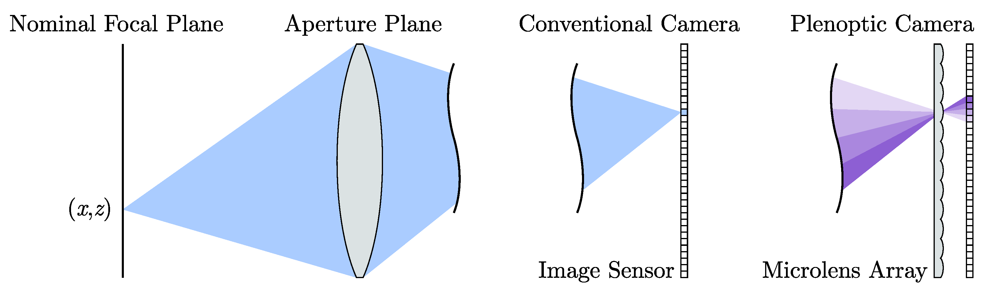
The plenoptic camera is a useful tool for flow diagnostics, since it enables the rapid acquisition of light-field data. As described by Levoy [37], a light field constitutes both the spatial and angular information about the light rays in a scene. Adelson and Wang [38] first introduced the modern concept of light-field imaging and the plenoptic camera in the early 1990s; they sought a way to advance imaging capabilities to capture more information about the light field. The physical advancement of plenoptic imaging was led by Ng et al. [15,39] in 2005 with the development of the handheld plenoptic camera. Ng describes the plenoptic camera’s most well-known ability to refocus and shift perspective of a scene computationally after the image has been captured. A plenoptic camera can be constructed by modifying a conventional camera to include an array of microlenses between the image sensor and the main lens. This microlens array changes how the light is focused on the image sensor, as shown in Figure 1. In a conventional camera, the main lens focuses light rays directly onto the image sensor. A plenoptic camera uses the main lens to focus light rays onto the microlens array. This, in turn, distributes the light rays onto the pixels of the image sensor depending on the angle the ray struck the microlens. In this way, a plenoptic camera encodes the angular information in addition to the spatial information for each light ray entering the camera. The result is a compact camera capable of sampling volumetric information in instantaneous snapshots, thereby enabling many possibilities in the realm of flow diagnostics. The Advanced Flow Diagnostics Laboratory (AFDL) of Auburn University has constructed many plenoptic cameras for use in PIV [16,17,18,19,20] and PTV [21,22,23], with a recent focus on scalar-field diagnostics, such as background-oriented schlieren [24], chemiluminescence [25], and pyrometry [25].
Although volumetric reconstructions can be performed using a thin-lens assumption, a volumetric calibration procedure provides many advantages. Direct light-field calibration (DLFC; [40]) is an empirical method to map object-space coordinates to image-space coordinates for each unique perspective . Similar to calibration procedures of other imaging techniques, a known calibration target is positioned successively throughout the volume, and its image-space coordinates are directly measured. A polynomial relationship between the known object coordinates and the measured image coordinates is then calculated using a least-squares solver. The resulting calibration polynomials correct for any optical distortions caused by lenses or facility windows, thereby enabling spatially accurate reconstructions. The calibration polynomials also provide a convenient way to calculate in Equations (2) and (3). Although this results in repeated operations, it greatly reduces memory requirements, since the relationship between every ith pixel and jth voxel is no longer necessary. Finally, the use of a global coordinate system enables multiple plenoptic cameras to reconstruct a single volume.
2.3. Plenoptic Spectral Imager
Danehy et al. have demonstrated three-color [27] and seven-color [28] pyrometry using a plenoptic camera. By inserting a series of color filters near the aperture plane of a plenoptic system, the authors were able to encode wavelength information into the perspective views. The resulting device is referred to as a plenoptic spectral imager (US Patent number 10,417,779 B2; [41]). The relationship between the encoded wavelengths was then used to deduce 2D maps of temperature and emissivity. In these works, the parallax between perspectives was assumed negligible, and thus the angular information was effectively traded for wavelength information. However, that is not strictly true: when imaging 3D scenes, the angular component still exists but is inextricably coupled with wavelength.
2.4. Volumetric Multispectral Measurements
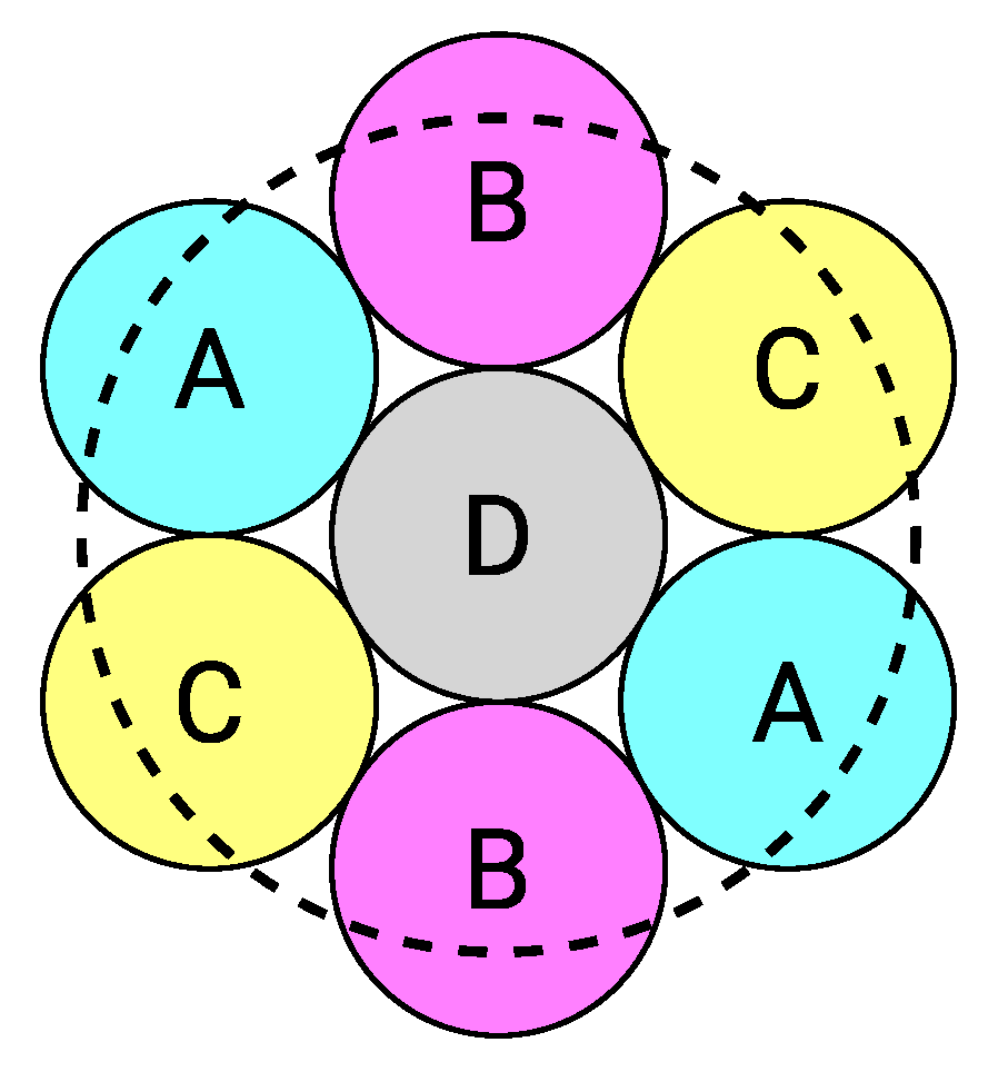
By introducing redundant filters into the plenoptic spectral imager, as shown in Figure 2, sufficient angular information should be retained to enable volumetric reconstruction. The dashed circle represents the aperture of a plenoptic camera. Any point within this circle may be used to generate a unique perspective. A set of points picked within like-colored filters would thus generate a set of perspectives associated with that color. As illustrated, filters A–C form stereo pairs that capture the maximum available parallax along one axis, which occurs from edge-to-edge for the aperture. The remaining filter D could remain neutral or broadband as a reference, replicate one of the other filters to bolster the corresponding reconstruction, or provide a fourth spectrum. If additional parallax is required, three filters per spectrum could be employed resulting in a triangular formation. Further optimization is possible with the construction of custom cut and coated filters; however, this study focuses on feasibility and thus restricts itself to commercial off-the-shelf filter choices.
Although these volumetric reconstructions will have reduced fidelity compared to utilizing the entire aperture, this method allows for simultaneous capture of multiple spectra per camera. The user may select all spectra freely as dictated by the needs of the experiment. This work seeks to (1) quantify reconstruction accuracy and (2) qualify reconstruction artifacts, each as a function of simultaneous spectra.
3. Methodology
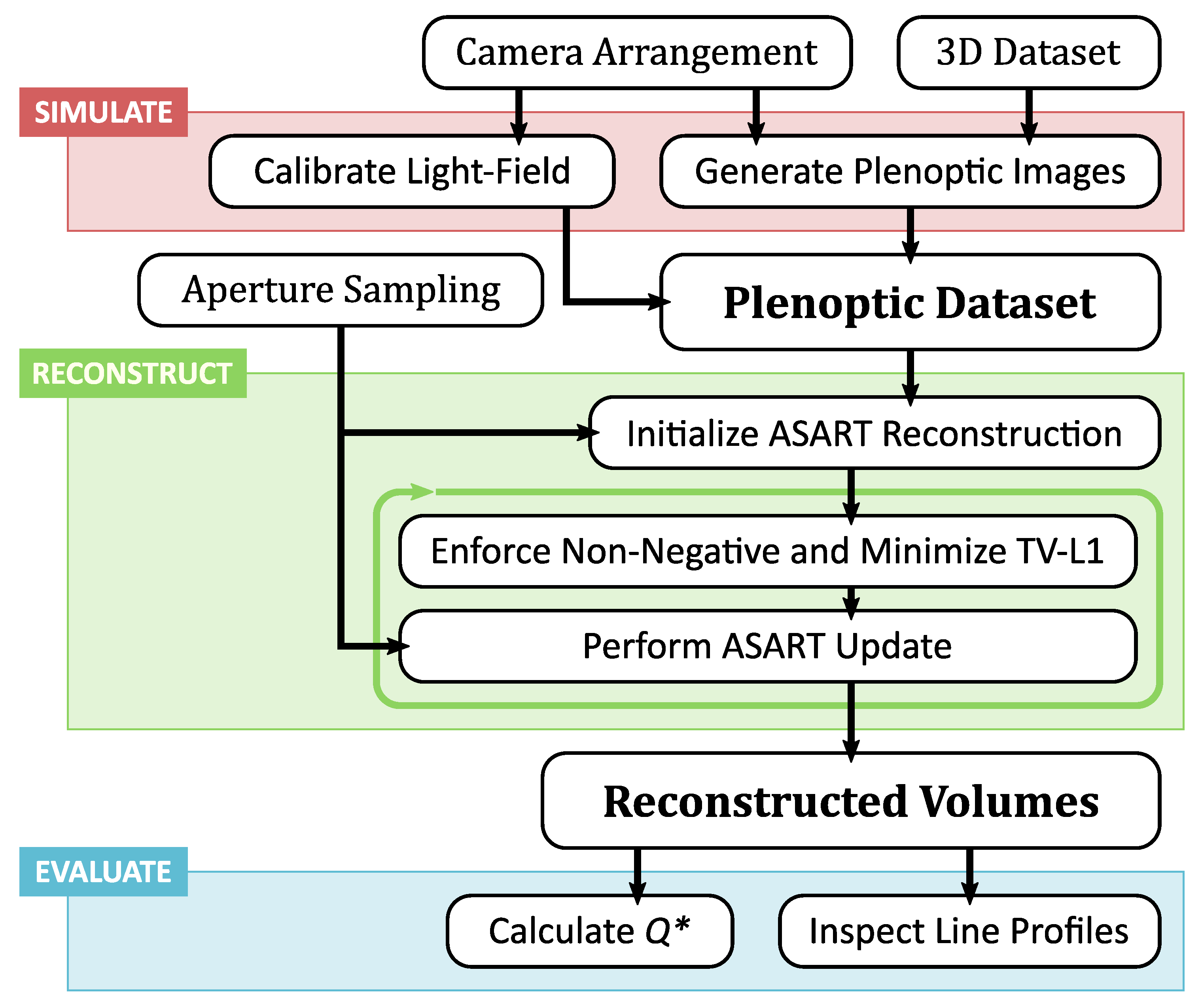
To obtain a quantitative measure of reconstruction accuracy, the true solution must be known; thus synthetic data was utilized for this study. The methodology of simulating, reconstructing, and evaluating that data is summarized in Figure 3. The remainder of this section serves to detail each step.
3.1. Simulation
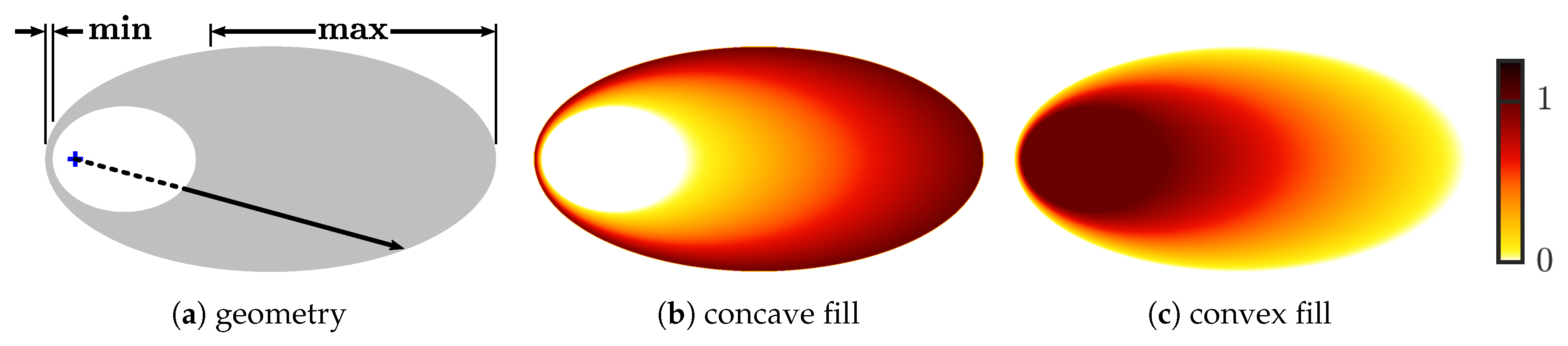
A 3D dataset with a prescribed range of features and length scales (hereafter referred to as a phantom) can be used to benchmark the reconstruction process. Many such phantoms exist in the medical imaging literature, such as the Shepp–Logan [42]. However, they do not suitably represent features commonly found in reacting flows, such as smooth gradients. The phantom crafted for this study was inspired by jet plumes. The construction of the phantom is illustrated in Figure 4 along with two example cross-sections. It is crafted from two ellipsoids sharing a common focal point. The intensity between ellipsoids is given by a linear ramp projected radially from the common focal point. The dimensions used here are 60 × 30 × 30 mm for the outer ellipsoid and 19 × 13.9 × 13.9 mm for the inner ellipsoid. The result is a continuous scalar field whose gradient magnitude spans 1.6 orders of magnitude between min and max, as shown. Line profiles through the focal point will always result in a top-hat function with sloped edges. Line profiles elsewhere through the volume will result in parabolic curves. In total, three variations of the phantom were considered: constant throughout, concave with null inner ellipsoid, and convex with uniform inner ellipsoid. Collectively, these phantoms represent a myriad of features and scales present in reacting flows and will help identify the limits of volumetric reconstruction.
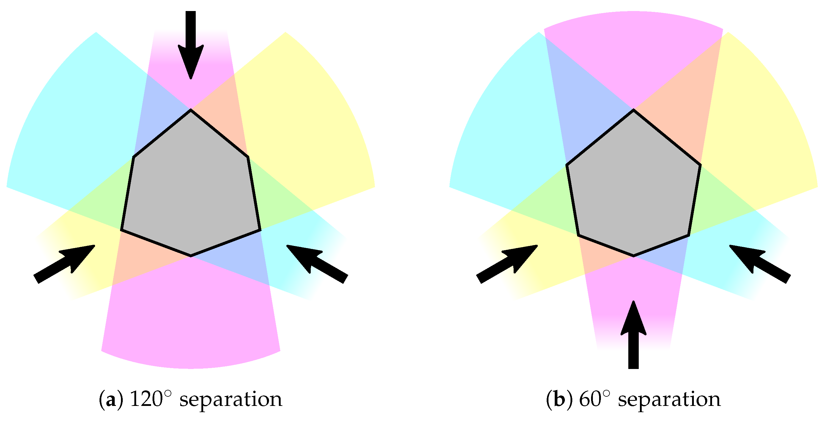
Both the number and arrangement of cameras are critical to the success of the reconstructions. Assuming an isotropic distribution of features, the ideal arrangement of cameras would surround the experimental volume in a spherical array. However, that is impractical from an experimental perspective, and the phantoms considered here are axisymmetric, similar to many reacting flows. Thus it was chosen to keep all cameras in a plane normal to the major axis to maximize the number of observations along the centerline. For an odd number of cameras n, the optimal in-plane rotation should be . A similar principle applies for an even number of cameras, but extra care must be taken to avoid collinear lines of sight, resulting in the “bent X” configuration common in four-camera tomo-PIV setups. An optimal three-camera arrangement is illustrated in Figure 5a. The intersection of all views is shown in gray and takes the shape of a non-regular hexagon with three orders of symmetry. Restricting the array to a semicircle results in angular separations of and is equivalent to inverting the position of every other camera. This limits the required optical access and has the added benefit of working equally well for an even or odd number of cameras. As illustrated in Figure 5b, similar lines of sight are achieved, but the intersection has only one order of symmetry. This bias towards the neighboring cameras could result in uneven reconstructions. However, complete optical access is not always possible or practical. Thus the limited-angle arrangement shown in Figure 5b is a better representation of real world experiments.
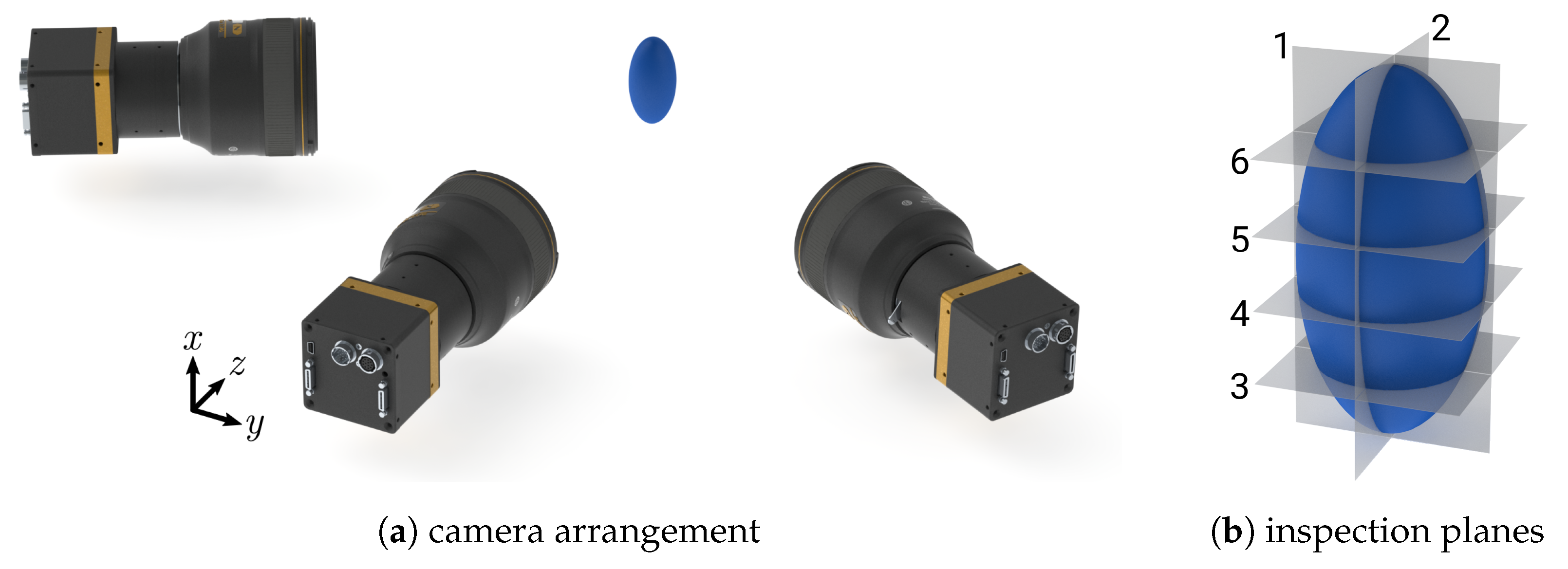
Plenoptic images of the phantoms were simulated on n cameras positioned in a linear array with separations, as illustrated in Figure 6. Linear arrays composed of two to six cameras were briefly evaluated. Three cameras should be shown to provide sufficient reconstruction fidelity while requiring only moderate optical access, and that is thus the focus of detailed study. The details of the synthetic plenoptic image generator are provided by Fahringer et al. [16]. The cameras used were Imperx Bobcat B6640 29 MP (6600 × 4400 pixels, 5.5 pixel pitch) housing a 471 × 362 hexagonally-packed microlens array with 77 pitch and 308 focal length. Each camera was equipped with a 60 mm main lens. The working distance from each camera to the center of the experimental volume was approximately 255 mm, resulting in a magnification of −0.5. The source grid was 60 × 30 × 30 mm and simulated with a resolution of 0.05 mm/cell. For each cell, 80 rays were propagated from a random point within the cell through the optics and onto the synthetic sensor. This resulted in a total of rays per image. The synthetic images were simulated at high spatial resolution to better approximate a continuous scalar field.
3.2. Reconstruction
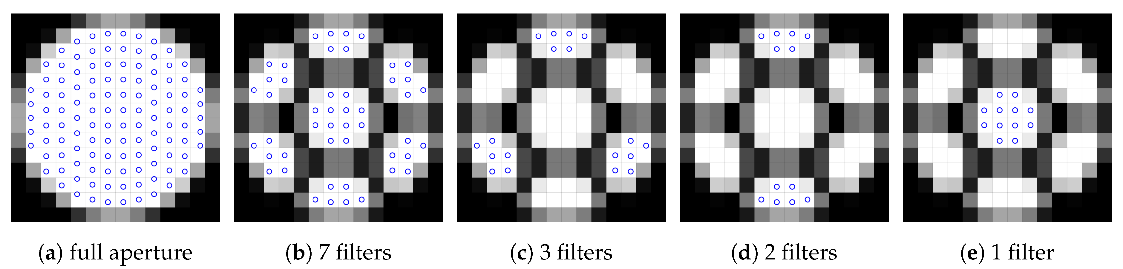
The aperture configurations considered here are illustrated in Figure 7, where each point represents a (u,v) coordinate associated with a unique perspective view. Note that the illustrated pixels are a nominal representation; the microlens array is not aligned with the sensor array, so each microlens will have a slightly different arrangement of pixels behind it. As such, the (u,v) samples are distributed to maximize the available parallax rather than align with underlying pixels. The appearance of the aperture is based carefully upon the experimental results of Fahringer et al. [28] using a plenoptic spectral imager. A total of five cases will be explored: (a) the full aperture, i.e., a typical plenoptic camera; (b) all seven filters for one spectra, providing a baseline for the mere insertion of the filter holder; (c) three filters per spectra, resulting in triangular triplets; (d) two filters per spectra, resulting in stereo pairs; and (e) one filter per spectra. If the samples are restricted to nominally unaffected pixels (i.e., white rather than gray or black), then only 48 valid samples remain after insertion of the multispectral component, greatly reducing the available samples even if all seven filters are utilized.
Reconstructions were performed using ASART+TV on a grid measuring 63 × 33 × 33 mm, slightly larger than the phantom. The nominal grid resolution is the size of one microlens (77 ) projected into object space, approximately 0.15 mm/vox here. The chosen grid resolution was 0.10 mm/vox. A key assumption made during both simulation and reconstruction is that the volume remain optically thin. This means that photons travel in a straight line to the main lens without encountering any refraction or absorption. To augment the reconstruction process, dynamic volume masking was utilized. A volume mask limits the scope of the reconstruction problem to a predefined region, which increases both accuracy and performance. For every instantaneous snapshot, each reconstructed voxel must contain some percentage of non-trivial observations. The noise floor and filter threshold are user-defined values of 10 counts and 92%, respectively. This mask shrink-wraps the data of a given snapshot. There are no convex-hull assumptions and the dynamic mask may have holes or discontinuities. These masks are binary, and merely inform on the reconstruction process which voxels are safe to skip. For complex scalar fields, masking is critical to the success of the reconstruction.
Volumetric calibration was performed via DLFC using a Monte Carlo simulation. One-thousand random points within the experimental volume were simulated and tracked with the plenoptic image generator. Using volumetric calibration in the synthetic tests alleviates the need to store and makes the processing procedure more analogous to real-world experiments.
3.3. Evaluation
The zero-mean reconstruction quality factor , as defined by La Foy and Vlachos [43], is used as an objective measure of the reconstruction. It is given by
where and are the zero-mean reconstructed scalar field and the zero-mean truth scalar field, respectively. A consequence of subtracting the mean is that large zero-valued regions increase ; thus, the quality factor could be artificially inflated by enlarging the reconstruction domain. To mitigate this trend, only voxels within the dynamic volume mask are used to calculate for each case. Note that although the phantom extents are identical in all cases, the dynamic masks vary slightly based on the observations available in each case. These quality factors are used to quantify the bulk accuracy of the reconstruction.
To assess small-scale features, cross-sectional planes of the reconstructed volume are extracted. Normalized coordinates are used, where at the base of the phantom and 1 at the top. A radial coordinate r in the y-z plane is 0 along the centerline and 1 at the major diameter (15 mm). Each plane is shown and labeled in Figure 6b. The first two correspond with the x-y and x-z cardinal planes, respectively. The remaining four are y-z planes positioned in 20% increments along the major axis. From these planes, false color maps of absolute intensity and full-scale error are presented in addition to individual line profiles.
4. Results and Discussion
4.1. Number of Cameras
Before beginning a detailed study, it is necessary to determine the appropriate number of cameras to utilize. A linear array of n cameras, separated by each, was simulated about the constant ellipsoid phantom. For this portion of the work, only 30 iterations of ASART were applied and no TV-L1 minimization was used. The results are therefore not converged, but serve as a representative sample.
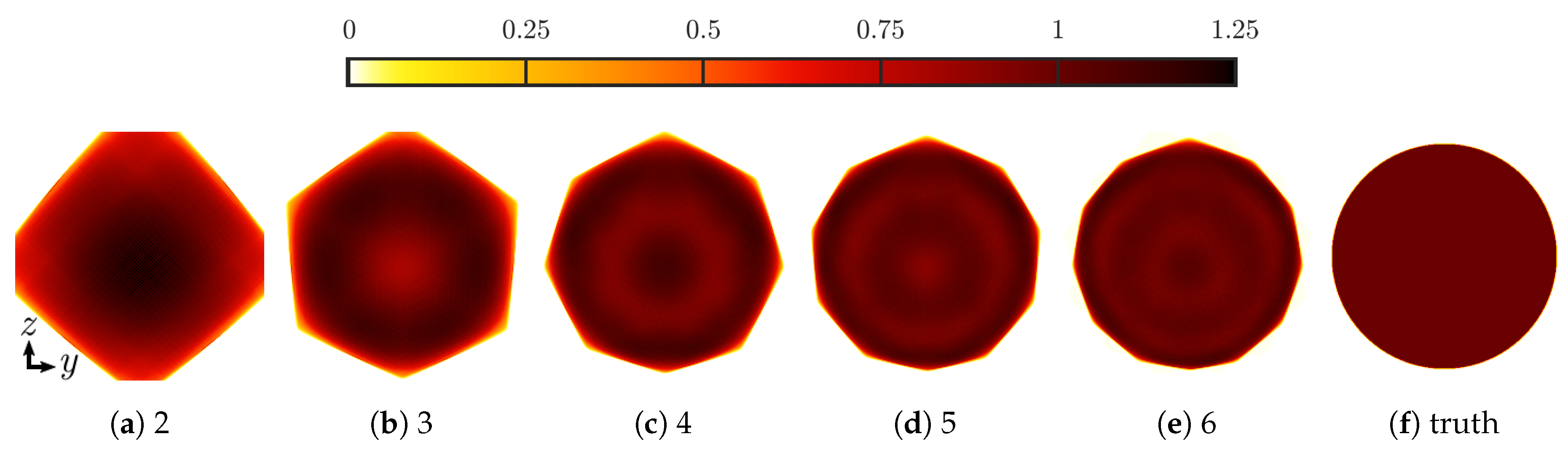
Cross-sections of the midplane are shown in Figure 8 for a number of cameras from two to six. As illustrated by Figure 8f, the cross-section should be a perfect circle with a value of unity. The outer boundary of each reconstruction is a lopsided polygon as predicted in Figure 5b, where the number of sides is . Note that in the two camera case, the corners are cropped by the reconstruction domain, making it falsely appear as an octagon. The polygonal boundaries are a product of trivial observations: outside of the boundary, there is high confidence that no real data exists because at least a few perspectives observe nothing in that region. With dynamic masking, this region is calculated as a preliminary step; however, the ASART algorithm is robust and will eventually accomplish the same task. Within the interior, an interference pattern based on n is observed. As the number of cameras increases, the interference pattern becomes more complex but of diminishing magnitude.
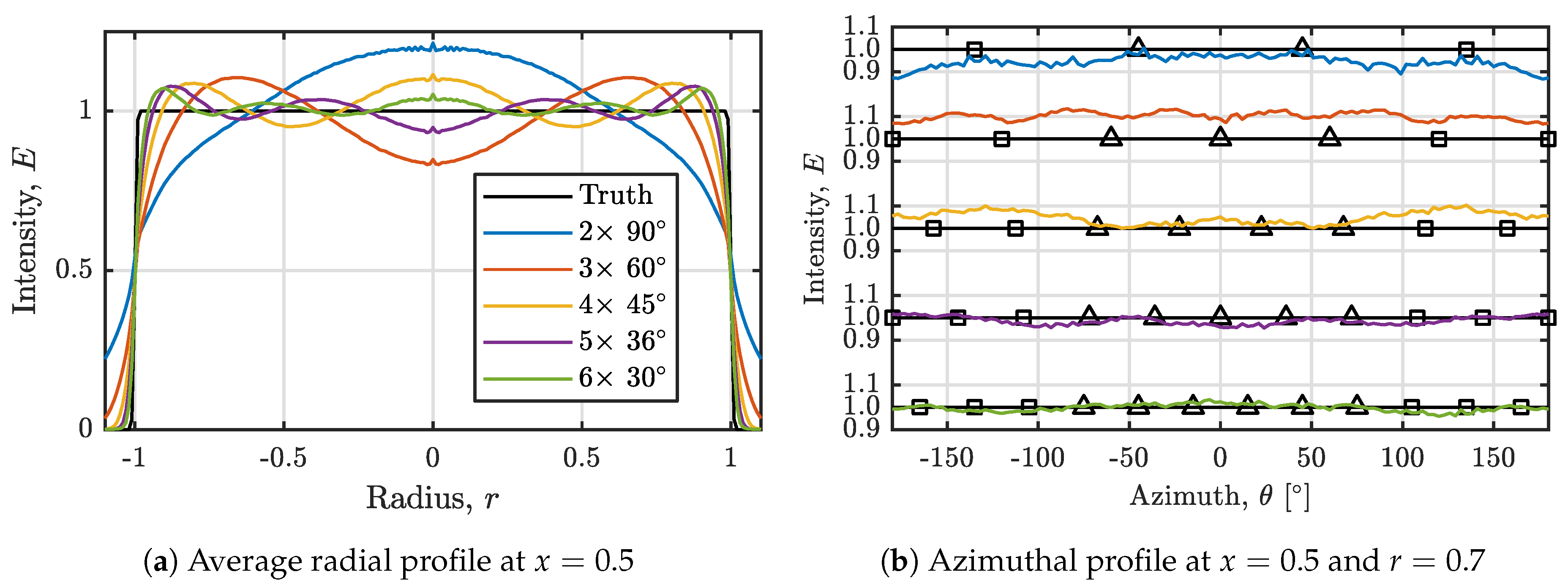
Average radial line profiles within the midplane are shown in Figure 9a for each linear array. The profiles resemble Fourier series approximations of a square wave. Increasing the number of cameras causes similar behavior to increasing the number of Fourier modes, gradually approaching the desired square profile. In the limit of many cameras, the oscillations are expected to become vanishingly small. Azimuthal () profiles within the midplane are shown in Figure 9b, along with symbols indicating where the primary axis of each camera enters (Δ) and exits (□) the volume. Note that at a fixed radius of , the azimuthal profiles do not necessarily correspond with a radial node or anti-node. Azimuthal oscillations are clearly observed as a function of n. The general trend, best illustrated by the three-camera case, is that each undulation directly correlates with a camera axis.
The source of this interference pattern is likely related to the hybrid nature of using multiple plenoptic cameras. The parallax between neighboring views is small, but the parallax between cameras is comparatively large. This causes a systematic bias in the distribution of energy throughout the reconstruction process. As the number of cameras increases, the separation between views becomes more uniform and the energy is more evenly distributed. These spatial oscillations were also observed when utilizing a variety of other reconstruction techniques, again suggesting that the bias is fundamental in nature. From these results it is obvious that the more cameras, the better. Further study is restricted to three cameras, which the authors believe provide sufficient fidelity while requiring only a moderate amount of optical access and experimental complexity.
4.2. Single Spectra Reconstructions Using the Full Aperture
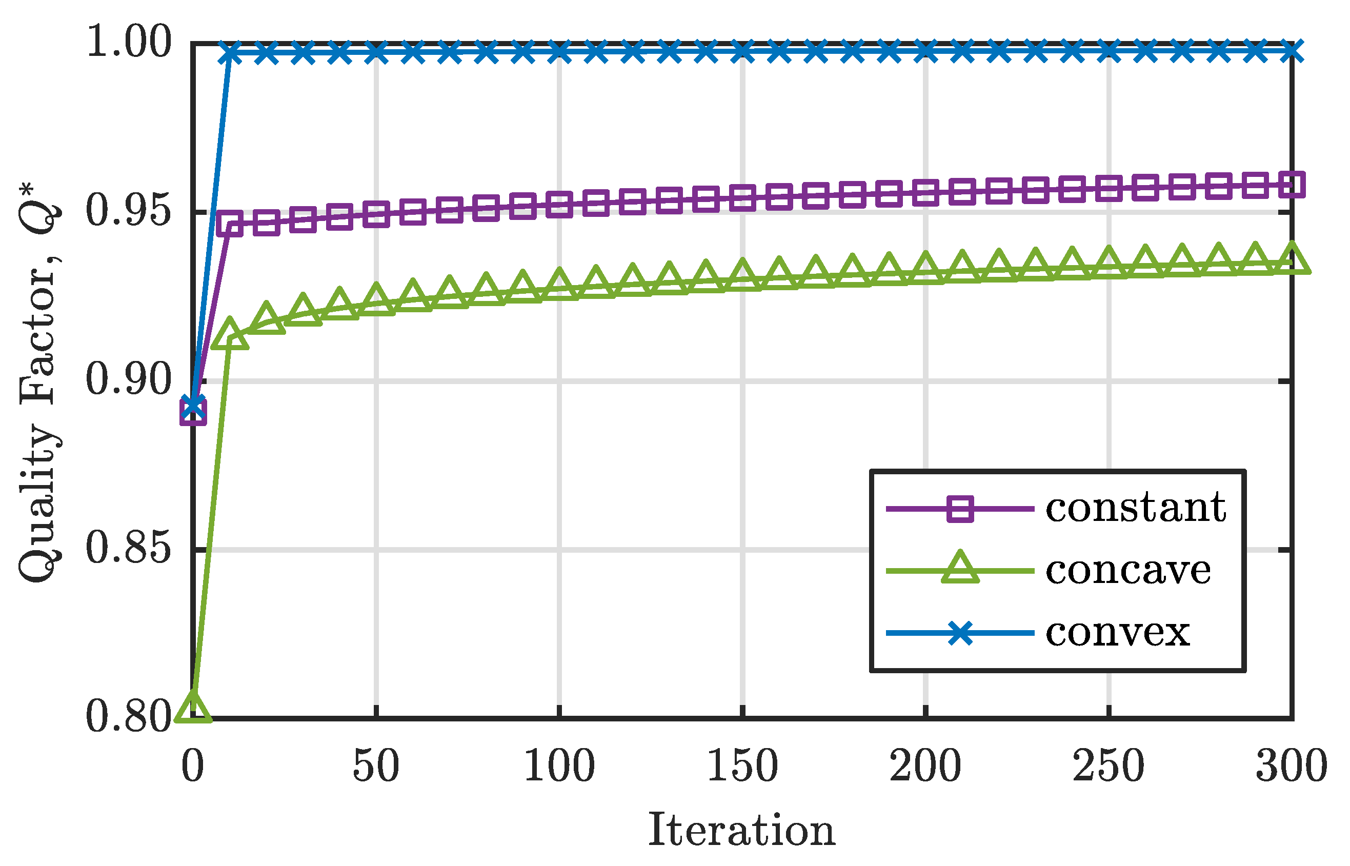
Based on the results of n cameras in a linear array, a three camera arrangement separated by 60 was chosen for detailed study. All three ellipsoid phantoms were reconstructed with ASART+TV using the full aperture (116 unique views) of each camera. These reconstructions provide a baseline by which the multispectral reconstructions may be compared. The quality factor of each phantom is shown in Figure 10 for every 10th iteration of the reconstruction process. At 300 iterations the quality is still improving and thus not fully converged; however, beyond 50 iterations the rate of change is quite slow. Therefore performing more than 300 iterations would be of marginal benefit and is not considered here.
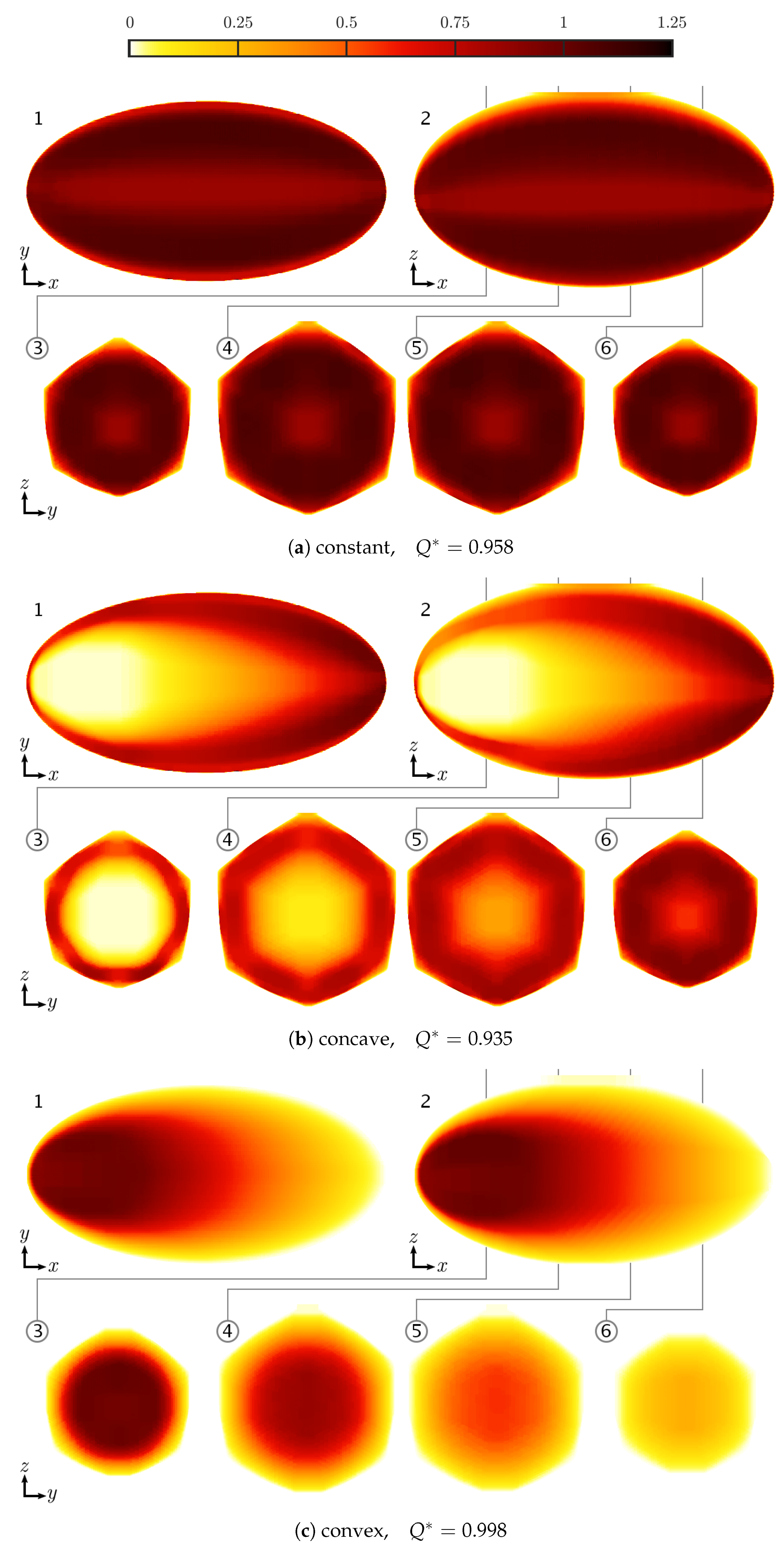
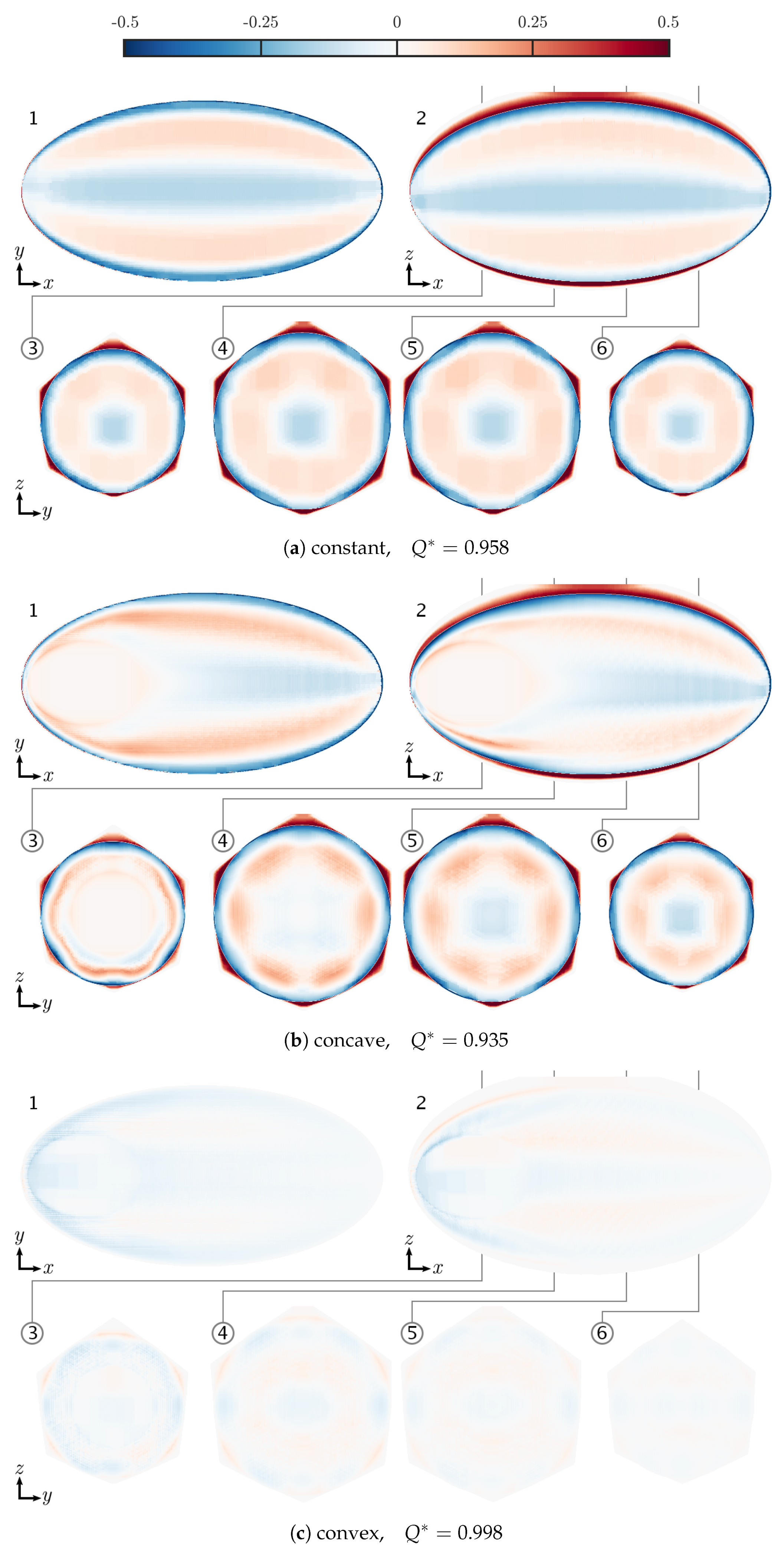
Cross-sections of the full-aperture reconstructions are shown in Figure 11. Several strengths and weaknesses are immediately evident. The hexagonal boundaries visible in the y-z cross-sections (planes 3–6) resemble Figure 5b as predicted. Although the outer boundaries are hexagonal, smooth and round features are observed within the interior. Overall, the reconstruction process faithfully recovers each phantom. Reconstruction of the convex phantom in particular exceptional with a quality factor of 0.998. All three phantoms exhibit a tube-shaped surplus along the major axis, although this is less evident in the convex case. This bias in energy distribution is directly related to the number of cameras, as was discussed in Section 4.1. Cross-sections of the full-scale error are shown in Figure 12 to highlight the differences. The error maps resemble a Fourier series, as was predicted in Figure 9a. However, the exact nature of the fluctuations vary with each phantom. The zero-valued hollow in the concave case appears to compress the fluctuations to the outermost edges, as shown in Figure 12b3. The remainder of the concave errors are more star-shaped than hexagonal. The convex error maps are similar to concave, but of substantially lesser magnitude. Although it would be preferable to eliminate these systematic biases, that is left for future research. For the remainder of this work, these errors will be taken as a predictable artifact of reconstruction.
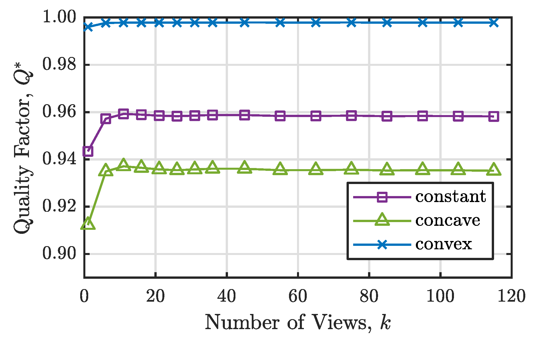
To explore the impact of view count, limited-view reconstructions were explored. All three ellipsoid phantoms were reconstructed with ASART+TV using the full aperture of each camera; however, the total number of views was limited to k points equally distributed about the aperture. Other distributions such as a ring about the aperture perimeter and a horizontal line were also considered, but were consistently out-performed by the equally distributed samples. Note that the resolution of each perspective view is fixed based on the number of microlenses; therefore, the system resolution increases linearly with the total number of views. It is thus natural to assume that more views will always yield superior results, since the number of observations per voxel is increasing. The resulting quality factors are presented in Figure 13. When , the system is effectively equivalent to three traditional (i.e., non-plenoptic) cameras with low resolution. Despite that limitation, fair reconstructions are still achieved. Reconstruction quality improves with additional views, peaking around then gradually settling from there. This could be related to the distribution of views discussed in Section 4.1. It is possible that a decrease in views per camera makes the overall distribution of views more uniform and thus benefits the reconstruction. Although these results do not reflect clustered-view distributions, as with the honeycomb filter, they indicate that utilizing all available views is unnecessary and somewhat detrimental. This gives confidence that the superfluous views may be utilized for other spectra with minimal sacrifices in quality.
4.3. Multispectral Reconstructions Using Honeycomb Aperture
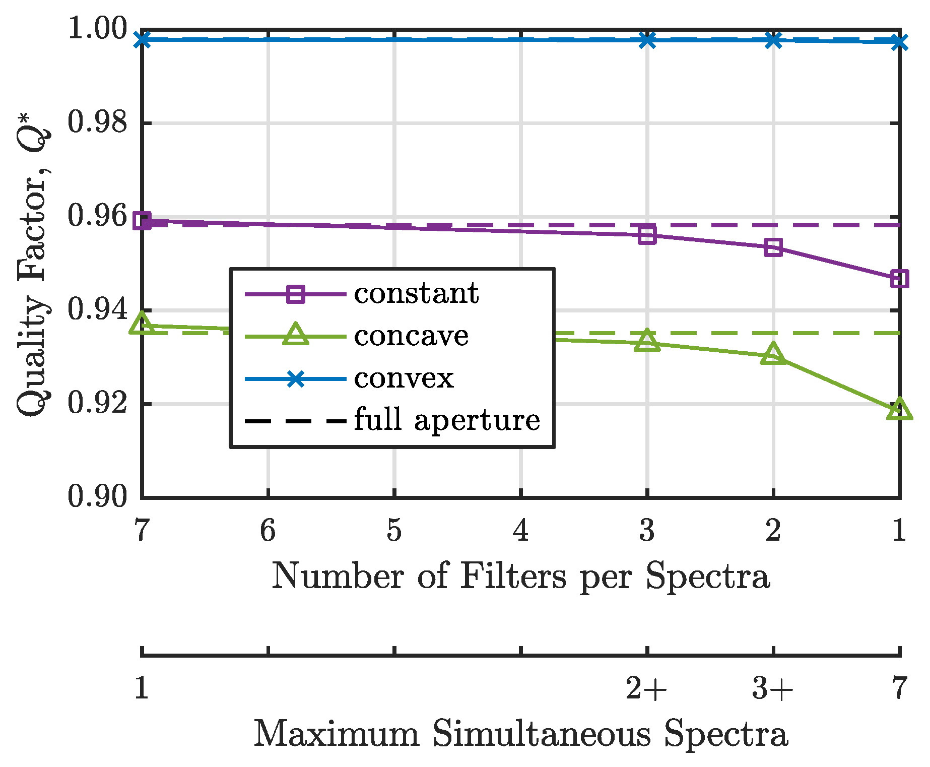
Using the previous full-aperture data, sub-aperture reconstructions were performed using a portion of the aperture representative of each configuration. This emulates the use of a multispectral lens without introducing additional complexity or error. The quality factor of each reconstruction is shown in Figure 14 for each aperture configuration. Varied orientations of each configuration (e.g., a horizontal stereo pair) were found to have the similar performances. Using seven filters has a slight benefit over the full aperture; similarly to Figure 13, reducing the number of views but maintaining the full span of the aperture appears to subtly improve reconstruction quality. However, this configuration serves only as a reference and provides no practical use; a reduction in views may be done during the reconstruction process and does not require any additional hardware. The three-filter configuration, which maximizes parallax in a triangular arrangement, performs comparably to the full aperture. Utilizing two filters in a stereo arrangement, and thus maximizing parallax across just one axis of the aperture, results in a marginal loss of quality. Finally, the one-filter configuration, which has the least parallax, performs the worst overall. Recall that for the two- and three-filter configurations, the central filter may be utilized for an additional spectra, albeit at lower quality. These results demonstrate that multiple spectra may be simultaneously acquired by a plenoptic camera array while still achieving fair reconstructions.
Once again, the distribution of views is important to consider alongside the number of views. The one-filter configuration utilizes 12 views and results in a concave quality factor of 0.918, compared to 0.937 for the reconstruction. However, the two and three-filter configurations, chosen to maximize parallax, perform favorably despite their limited view count. An optimized system should strive for a uniform distribution of views spanning a large range of angles.
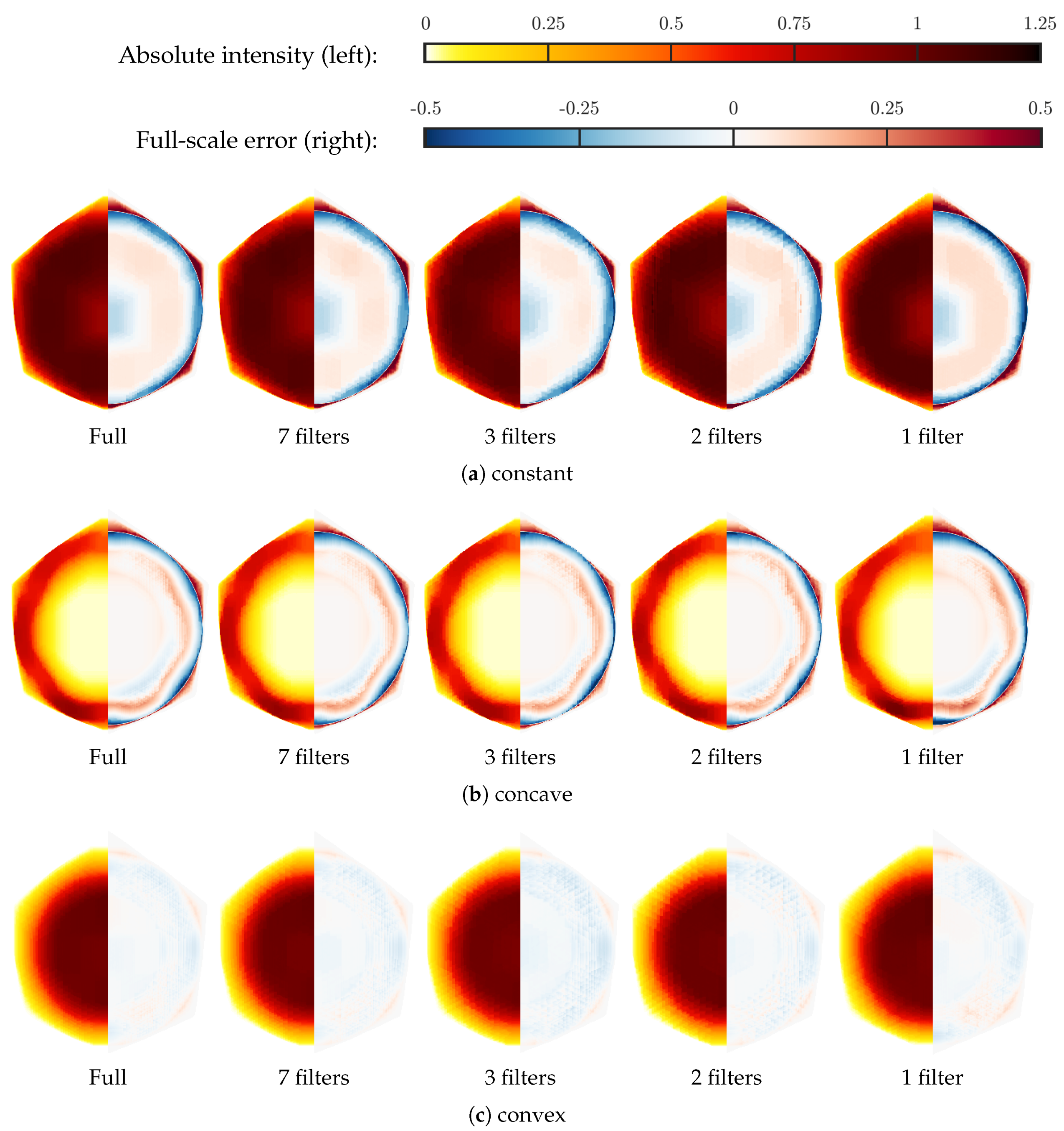
A subset of the multispectral reconstructions were chosen to illustrate the associated reconstruction artifacts. Cross-sections at plane 3 () of the multispectral reconstructions are shown in Figure 15 with false color for both absolute intensity (left) and full-scale error (right). The differences are subtle, but that was expected based on the quality factors. As the number of utilized filters decreases (thus enabling more simultaneous spectra), several aspects of the reconstruction degrade. The overall shape becomes less circular, with the boundary edges becoming sharper and trending toward a lopsided hexagon. Internally, the features also become less circular and more egg-shaped. The distribution of intensity loses its smoothness and becomes increasingly noisy. In particular, a stair step pattern emerges that is especially visible near the perimeter. The edges of each step are triangular and aligned with the camera axes.
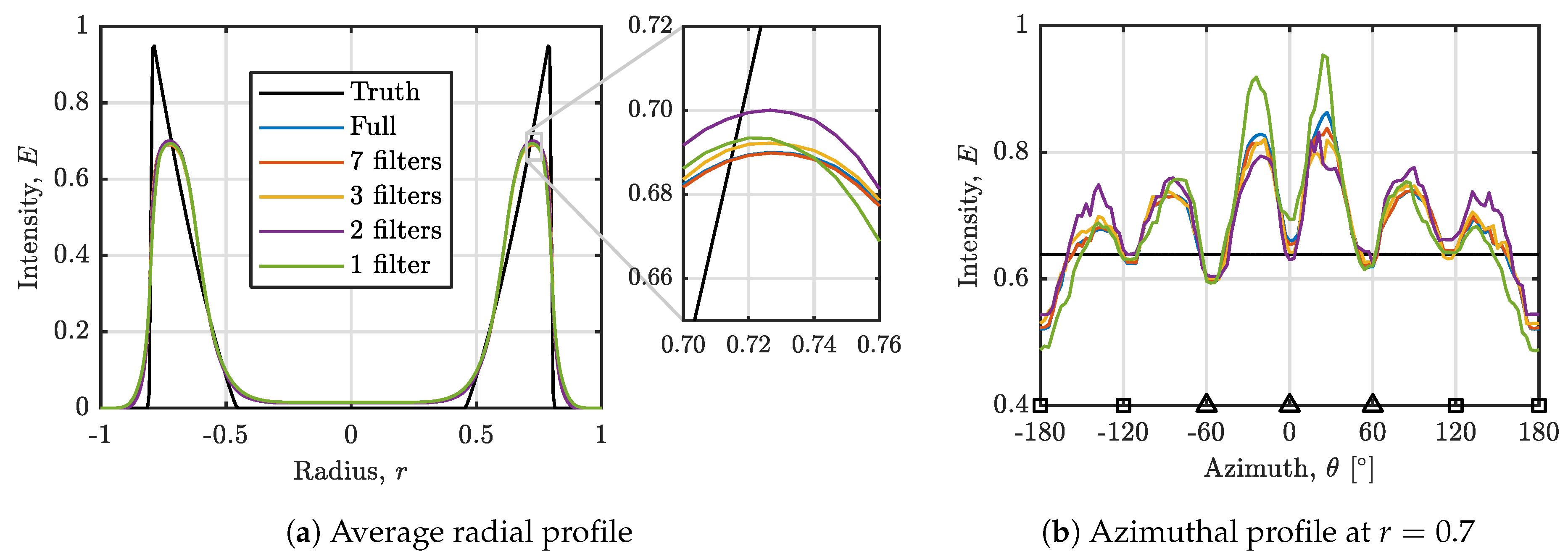
To better illustrate the magnitude associated with these reconstruction errors, line profiles within plane 3 of the concave reconstruction are shown in Figure 16. From the average radial profiles in Figure 16a, it is evident that all aperture configurations struggle to capture the sharp edge of the concave profile, but none stand out from the rest. An inset of the apex highlights how similarly all configurations perform. Azimuthally, six undulations are clearly observed, which correlate with the nominal axes of each camera. Compared to the constant phantom (whose line profiles are not shown), the compression of intensity amplifies the magnitude of these fluctuations. The 1-filter configuration deviates from the truth most dramatically, with peaks and troughs of the greatest magnitude. The other configurations are more similar to one another. The 2-filter configuration interestingly has undulations of lesser magnitude near , but of greater magnitude elsewhere.
5. Conclusions
The core of this work is to leverage the abundance of unique perspective views with the insertion of multiple filters at the aperture plane. As was shown in Figure 13, some of the full-aperture views may be sacrificed with little to no detriment. Rather than waste redundant views, the aperture was divided into seven regions using off-the-shelf components, enabling the simultaneous capture of up to seven different user-selected spectra. Since the accuracy of reconstructed features is known to scale with the available angular information, the proposed filter configurations were chosen to maintain maximum parallax.
A summary of the quality factors for each phantom reconstructed using ASART+TV is provided in Table 1. Overall, reconstructions closely resembling the three phantoms were achieved for all cases. At present, the largest source of error is directly related to the shape of the phantom. Reconstructions performed exceptionally for the convex phantom, but struggled with the constant and concave phantoms, particularly near the perimeter where intensity is discontinuous. Although gradients and internal hollows were well captured where present, the infinite gradient at the edge was problematic. Related to this, the second largest source of error appears to be a systematic bias based on the non-uniform distribution of views. A spatially-oscillating intensity, which resembled a Fourier series approximation, was observed based on the number of cameras. Using more cameras increased the spatial frequency and decreased the magnitude, similarly to increasing the number of Fourier modes, producing more accurate reconstructions. Although this work focused on the use of a plenoptic camera, other light-field imaging devices such as quad-scopes and fiber-optic bundles are expected to be similarly impacted.
Relative to those fundamental error sources, dividing the aperture into multiple spectra had a considerably lesser impact on reconstruction. It was discovered that utilizing all available views per camera was slightly detrimental to the reconstruction. Perhaps related to the distribution of views and Fourier-like oscillations, utilizing fewer views but maintaining the full aperture had a marginal but positive effect on reconstruction quality. Insertion of the filter holder performed similarly to these limited-view reconstructions for all three phantoms. Using fewer filters and thus enabling more simultaneous spectra had a detrimental effect, but the overall loss in quality was significantly less than the gain in information. When partnered with complex and expensive-to-operate facilities, the capability to acquire up to seven hand-picked spectra far outweighs the small loss in quality.
Multispectral volumetric imaging is a largely unexplored frontier, providing a tremendous amount future work. An immediate focus should be placed on understanding and minimizing the systematic errors that cause spatially-oscillating features. A detailed Fourier domain analysis might reveal additional insights relating to the optimal arrangement for a limited number of views, which would be relevant for all light-field imaging systems. More elaborate 3D phantoms featuring asymmetries, azimuthal variations, and small-scale particulate matter would better represent turbulent reacting flows. Such phantoms, which can be achieved through CFD rather than manual crafting, will provide a necessary benchmark as this technology progresses. Physical construction of these multispectral imagers is underway and experimental studies will follow.
Author Contributions
Conceptualization, C.J.C. and B.S.T.; methodology, C.J.C.; software, C.J.C.; validation, C.J.C.; formal analysis, C.J.C.; investigation, C.J.C.; resources, C.J.C. and B.S.T.; data curation, C.J.C.; writing—original draft preparation, C.J.C.; writing—review and editing, C.J.C. and B.S.T.; visualization, C.J.C.; supervision, B.S.T.; project administration, B.S.T.; funding acquisition, C.J.C. and B.S.T. All authors have read and agreed to the published version of the manuscript.
Funding
This material is based upon work sponsored by the Army SBIR Program Office under Contract No. W31P4Q-19-P=0047 through a subcontract from MetroLaser Inc. Any opinions, findings, and conclusions or recommendations expressed in this material are those of the author(s) and do not necessarily reflect the views of the Army SBIR Office.
Acknowledgments
This work was completed in part with resources provided by the Auburn University Hopper Cluster.
Conflicts of Interest
The authors declare no conflict of interest.
References
- Scarano, F. Tomographic PIV: Principles and practice. Meas. Sci. Technol. 2013, 24, 012001. [Google Scholar] [CrossRef]
- Coriton, B.; Steinberg, A.M.; Frank, J.H. High-speed tomographic PIV and OH PLIF measurements in turbulent reactive flows. Exp. Fluids 2014, 55. [Google Scholar] [CrossRef]
- Boxx, I.; Carter, C.; Meier, W. On the feasibility of tomographic-PIV with low pulse energy illumination in a lifted turbulent jet flame. Exp. Fluids 2014, 55. [Google Scholar] [CrossRef] [Green Version]
- Weinkauff, J.; Michaelis, D.; Dreizler, A.; Böhm, B. Tomographic PIV measurements in a turbulent lifted jet flame. Exp. Fluids 2013, 54. [Google Scholar] [CrossRef]
- Xie, T.; Mukai, D.; Guo, S.; Brenner, M.; Chen, Z. Fiber-optic-bundle-based optical coherence tomography. Opt. Lett. 2005, 30, 1803–1805. [Google Scholar] [CrossRef] [PubMed]
- Ford, H.D.; Tatam, R.P. Fibre imaging bundles for full-field optical coherence tomography. Meas. Sci. Technol. 2007, 18. [Google Scholar] [CrossRef]
- Liu, H.; Shui, C.; Cai, W. Time-resolved three-dimensional imaging of flame refractive index via endoscopic background-oriented Schlieren tomography using one single camera. Aerosp. Sci. Technol. 2020, 97, 1–7. [Google Scholar] [CrossRef]
- Halls, B.R.; Thul, D.J.; Michaelis, D.; Roy, S.; Meyer, T.R.; Gord, J.R. Single-shot, volumetrically illuminated, three-dimensional, tomographic laser-induced-fluorescence imaging in a gaseous free jet. Opt. Lett. 2016, 24, 1–10. [Google Scholar] [CrossRef]
- Halls, B.R.; Hsu, P.S.; Jiang, N.; Legge, E.S.; Felver, J.J.; Slipchenko, M.N.; Roy, S.; Meyer, T.R.; Gord, J.R. kHz-rate four-dimensional fluorescence tomography using an ultraviolet-tunable narrowband burst-mode optical parametric oscillator. Optica 2017, 4, 897–902. [Google Scholar] [CrossRef]
- Lauriola, D.K.; Gomez, M.; Slipchenko, M.N.; Son, S.F.; Meyer, T.R.; Roy, S.; Gord, J.R. kHz–MHz Rate Laser-Based Tracking of Particles and Product Gases for Multiphase Blast Fields. In Proceedings of the 2018 IEEE Research and Applications of Photonics In Defense Conference (RAPID), Mirimar Beach, FL, USA, 22–24 August 2018; pp. 1–4. [Google Scholar]
- Lauriola, D.K.; Gomez, M.; Meyer, T.R.; Son, S.F.; Slipchenko, M.N.; Roy, S. High-Speed Particle Image Velocimetry and Particle Tracking Methods in Reactive and Non-Reactive Flows. In Proceedings of the AIAA Scitech 2019 Forum, San Diego, CA, USA, 7–11 January 2019. Number 2019-1605. [Google Scholar] [CrossRef]
- Halls, B.R.; Hsu, P.; Legge, E.; Roy, S.; Meyer, T.R.; Gord, J.R. 3D OH LIF Measurements in a Lifted Flame. In Proceedings of the 55th AIAA Aerospace Sciences Meeting, Grapevine, TX, USA, 9–13 January 2017. Number 2017-1646. [Google Scholar] [CrossRef]
- Halls, B.R.; Gord, J.R.; Hsu, P.; Roy, S.; Meyer, T.R. Development of Two-Color 3d Tomographic VLIF Measurements. In Proceedings of the 2018 AIAA Aerospace Sciences Meeting, Kissimmee, FL, USA, 7–12 January 2018. Number 2018-1022. [Google Scholar] [CrossRef]
- Halls, B.R.; Hsu, P.S.; Roy, S.; Meyer, T.R.; Gord, J.R. Two-color volumetric laser-induced fluorescence for 3D OH and temperature fields in turbulent reacting flows. Opt. Lett. 2018, 43, 2961–2964. [Google Scholar] [CrossRef]
- Ng, R. Digital Light Field Photography. Ph.D. Thesis, Stanford University, Stanford, CA, USA, 2006. [Google Scholar]
- Fahringer, T.W.; Lynch, K.P.; Thurow, B.S. Volumetric particle image velocimetry with a single plenoptic camera. Meas. Sci. Technol. 2015, 26, 115201. [Google Scholar] [CrossRef]
- Fahringer, T.W.; Thurow, B.S. Filtered refocusing: A volumetric reconstruction algorithm for plenoptic-PIV. Meas. Sci. Technol. 2016, 27, 094005. [Google Scholar] [CrossRef]
- Johnson, K.C.; Thurow, B.S.; Kim, T.; Blois, G.; Christensen, K.T. Volumetric velocity measurements in the wake of a hemispherical roughness element. AIAA J. 2017, 55. [Google Scholar] [CrossRef]
- Fahringer, T.W.; Thurow, B.S. Plenoptic particle image velocimetry with multiple plenoptic cameras. Meas. Sci. Technol. 2018, 29, 075202. [Google Scholar] [CrossRef]
- Raghav, V.; Clifford, C.; Midha, P.; Okafor, I.; Thurow, B.; Yoganathan, A. Three-dimensional extent of flow stagnation in transcatheter heart valves. R. Soc. Interface 2019, 16, 20190063. [Google Scholar] [CrossRef] [PubMed] [Green Version]
- Hall, E.M.; Guildenbecher, D.R.; Thurow, B.S. Uncertainty characterization of particle lcoation from refocused plenoptic images. Opt. Express 2017, 25. [Google Scholar] [CrossRef] [PubMed]
- Hall, E.M.; Guildenbecher, D.R.; Thurow, B.S. Development and uncertainty characterization of 3D particle location from perspective shifted plenoptic images. Opt. Express 2019, 27, 7997–8010. [Google Scholar] [CrossRef] [PubMed]
- Clifford, C.; Tan, Z.P.; Hall, E.; Thurow, B. Particle Matching and Triangulation using Light-Field Ray Bundling. In Proceedings of the 13th International Symposium on Particle Image Velocimetry, Munich, Germany, 22–24 July 2019. [Google Scholar]
- Klemkowsky, J.N.; Clifford, C.J.; Bathel, B.F.; Thurow, B.S. A direct comparison between conventional and plenoptic background oriented schlieren imaging. Meas. Sci. Technol. 2019, 30. [Google Scholar] [CrossRef]
- George, J.; Clifford, C.; Jenkins, T.; Thurow, B. Volumetric spectral imaging and two-color pyrometry of flames using plenoptic cameras. Proc. SPIE 2019, 11102, 1110216. [Google Scholar] [CrossRef]
- Meng, L.; Sun, T.; Kosoglow, R.; Berkner, K. Evaluation of multispectral plenoptic camera. Proc. SPIE 2013, 8660, 86600D. [Google Scholar] [CrossRef]
- Danehy, P.M.; Hutchins, W.D.; Fahringer, T.; Thurow, B.S. A Plenoptic Multi-Color Imaging Pyrometer. In Proceedings of the 55th AIAA Aerospace Sciences Meeting, Grapevine, TX, USA, 9–13 January 2017. Number 2017-1645. [Google Scholar] [CrossRef] [Green Version]
- Fahringer, T.W.; Danehy, P.M.; Hutchins, W.D. Design of a multi-Color Plenoptic Camera for Snapshot Hyperspectral Imaging. In Proceedings of the 2018 Aerodynamic Measurement Technology and Ground Testing Conference, Atlanta, GA, USA, 25–29 June 2018. Number 2018-3627. [Google Scholar] [CrossRef]
- Doster, T.; Olson, C.C.; Fleet, E.; Yetzbacher, M.; Kanaev, A.; Lebow, P.; Leathers, R. Designing manufacturable filters for a 16-band plenoptic camera using differential evolution. Proc. SPIE 2017, 10198, 1019803. [Google Scholar] [CrossRef]
- Xiong, Z.; Wang, L.; Li, H.; Liu, D.; Wu, F. Snapshot Hyperspectral Light Field Imaging. In Proceedings of the IEEE Conference on Computer Vision and Pattern Recognition, Honolulu, HI, USA, 21–26 July 2017; pp. 3270–3278. [Google Scholar]
- Kelly, D.; Phillips, M.; Clifford, C.; Scarborough, D.; Thurow, B. Novel Multi-band Plenoptic Pyrometer used for Termperature Measurements of Strand Burner Plumes. In Proceedings of the AIAA SciTech 2020 Forum, Orlando, FL, USA, 6–10 January 2020. Number 2020-1515. [Google Scholar] [CrossRef]
- Herman, G.T.; Lent, A. Iterative reconstruction algorithms. Comput. Biol. Med. 1976, 6, 273–294. [Google Scholar] [CrossRef]
- Wan, X.; Zhang, F.; Chu, Q.; Zhang, K.; Sun, F.; Yuan, B.; Liu, Z. Three-dimensional reconstruction using an adaptive simultaneous algebraic reconstruction technique in electron tomography. J. Struct. Biol. 2011, 175, 277–287. [Google Scholar] [CrossRef] [PubMed]
- Gordon, R. A tutorial on ART (algebraic reconstruction technique). IEEE Trans. Nucl. Sci. 1974, 21, 78–93. [Google Scholar] [CrossRef]
- Boyd, S.P.; Vandenberghe, L. Convex Optimization; Cambridge University Press: Cambridge, UK, 2004. [Google Scholar]
- Yang, S.; Wang, J.; Fan, W.; Zhang, X.; Wonka, P.; Ye, J. An Efficient ADMM Algorithm for Multidimensional Anisotropic Total Variation Regularization Problems. In Proceedings of the 19th ACM SIGKDD International Conference on Knowledge Discovery and Data Mining, KDD ’13, Chicago, IL, USA, 11–14 August 2013; ACM: New York, NY, USA, 2013; pp. 641–649. [Google Scholar] [CrossRef] [Green Version]
- Levoy, M. Light fields and computational imaging. Computer 2006, 39, 46–55. [Google Scholar] [CrossRef]
- Adelson, E.H.; Wang, J.Y.A. Single Lens Stereo with a Plenoptic Camera. IEEE Trans. Pattern Anal. Mach. Intell. 1992, 14, 99–106. [Google Scholar] [CrossRef] [Green Version]
- Ng, R.; Levoy, M.; Bredif, M.; Duval, G.; Horowitz, M.; Hanrahn, P. Light Field Photography with a Hand-Held Plenoptic Camera; Stanford Technical Report; Stanford University: Stanford, CA, USA, 2005. [Google Scholar]
- Hall, E.M.; Fahringer, T.W.; Thurow, B.S.; Guildenbecher, D.R. Volumetric calibration of a plenoptic camera. In Proceedings of the 55th AIAA Aerospace Sciences Meeting, Grapevine, TX, USA, 9–13 January 2017. Number 2017-1642. [Google Scholar] [CrossRef]
- Danehy, P.M.; Thurow, B.S. Methods and Systems for Processing Plenoptic Images. U.S. Patent United States 010417779 B2, 17 September 2019. Previously US 2018/0005402 A1. [Google Scholar]
- Shepp, L.A.; Logan, B.F. The Fourier Reconstruction of a Head Section. IEEE Trans. Nuclear Sci. 1974, NS-21, 21–43. [Google Scholar] [CrossRef]
- La Foy, R.R.; Vlachos, P. Multi-Camera Plenoptic Particle Image Velocimetry. In Proceedings of the 10th International Symposium on Particle Image Velocimetry, Delft, The Netherlands, 2–4 July 2013. [Google Scholar]
Figure 1.
Light-field sampling of conventional and plenoptic cameras.

Figure 2.
Filter arrangement at the main lens aperture plane.

Figure 3.
Flow chart of the data generation and evaluation process.

Figure 4.
Construction of the double ellipsoid phantom.

Figure 5.
Comparison of three-camera arrangements.

Figure 6.
Arrangement of the synthetic experiment.

Figure 7.
Multispectral aperture configurations chosen for comparison.

Figure 8.
Midplane of constant phantom reconstruction using n cameras.

Figure 9.
Line profiles of constant phantom reconstruction using n cameras.

Figure 10.
Convergence of quality factor using ASART+TV.

Figure 11.
Cross-sections of the full-aperture reconstructions.

Figure 12.
Cross-sections of the full-aperture reconstruction error.

Figure 13.
Quality factor with a limited number of views.

Figure 14.
Quality factor using a multispectral aperture.

Figure 15.
Cross-sections of the multispectral reconstructions at plane 3.

Figure 16.
Line profiles of concave phantom reconstruction at plane 3.


Table 1.
Quality factors for each aperture configuration.
| Config. | Views | Constant | Concave | Convex |
|---|---|---|---|---|
| Full | 116 | 0.958 | 0.935 | 0.998 |
| Best | ∼10 | 0.959 | 0.937 | 0.998 |
| 7 filters | 48 | 0.959 | 0.937 | 0.998 |
| 3 filters | 18 | 0.956 | 0.933 | 0.998 |
| 2 filters | 12 | 0.954 | 0.930 | 0.998 |
| 1 filter | 12 | 0.947 | 0.918 | 0.997 |
© 2020 by the authors. Licensee MDPI, Basel, Switzerland. This article is an open access article distributed under the terms and conditions of the Creative Commons Attribution (CC BY) license (http://creativecommons.org/licenses/by/4.0/).
Share and Cite
MDPI and ACS Style
Clifford, C.J.; Thurow, B.S. On the Impact of Subaperture Sampling for Multispectral Scalar Field Measurements. Optics 2020, 1, 136-154. https://0-doi-org.brum.beds.ac.uk/10.3390/opt1010010
AMA Style
Clifford CJ, Thurow BS. On the Impact of Subaperture Sampling for Multispectral Scalar Field Measurements. Optics. 2020; 1(1):136-154. https://0-doi-org.brum.beds.ac.uk/10.3390/opt1010010
Chicago/Turabian StyleClifford, Christopher J., and Brian S. Thurow. 2020. "On the Impact of Subaperture Sampling for Multispectral Scalar Field Measurements" Optics 1, no. 1: 136-154. https://0-doi-org.brum.beds.ac.uk/10.3390/opt1010010