Optical Measurements on Thermal Convection Processes inside Thermal Energy Storages during Stand-By Periods


Institute of Thermodynamics and Fluid Mechanics, Technische Universität Ilmenau, Am Helmholtzring 1, 98693 Ilmenau, Germany
*
Authors to whom correspondence should be addressed.
Optics 2020, 1(1), 155-172; https://0-doi-org.brum.beds.ac.uk/10.3390/opt1010011
Submission received: 26 March 2020
/
Revised: 17 April 2020
/
Accepted: 27 April 2020
/
Published: 29 April 2020
(This article belongs to the Special Issue Optical Diagnostics in Engineering)
Abstract
:Thermal energy storages (TES) are increasingly important for storing energy from renewable energy sources. TES that work with liquid storage materials are used in their most efficient way by stratifying the storage fluid by its thermal density gradient. Mixing of the stratification layers during stand-by periods decreases the thermal efficiency of the TES. Tank sidewalls, unlike the often poorly heat-conducting storage fluids, promote a heat flux from the hot to the cold layer and lead to thermal convection. In this experimental study planar particle image velocimetry (PIV) measurements and background-oriented schlieren (BOS) temperature measurements are performed in a model experiment of a TES to characterise the influence of the thermal convection on the stratification and thus the storage efficiency. The PIV results show two vertical, counter-directed wall jets that approach in the thermocline between the stratification layers. The wall jet in the hot part of the thermal stratification shows compared to the wall jet in the cold region strong fluctuations in the vertical velocity, that promote mixing of the two layers. The BOS measurements have proven that the technique is capable of measuring temperature fields in thermally stratified storage tanks. The density gradient field as an intermediate result during the evaluation of the temperature field can be used to indicate convective structures that are in good agreement to the measured velocity fields.
1. Introduction
Energy storage facilities as part of renewable power plants become increasingly important to achieve the aim of limiting the climate change [1] and guaranteeing a stable power grid at the same time [2,3,4]. Since a major part of global primary energy consumption is consumed or wasted as heat [5], thermal energy storage systems (TES) have the potential to become one of the most widespread energy storage technologies in the future. They can compensate for the disadvantages of other energy storage technologies such as electric batteries, pumped hydro storages or compressed air energy storages by the fact that they usually consist of relatively cheap construction and storage materials and do not have to meet any geological restrictions [3,4,6,7]. For this reason, TES have been a part of numerous scientific studies in the field of energy storage in recent years [8,9,10,11,12,13,14,15].
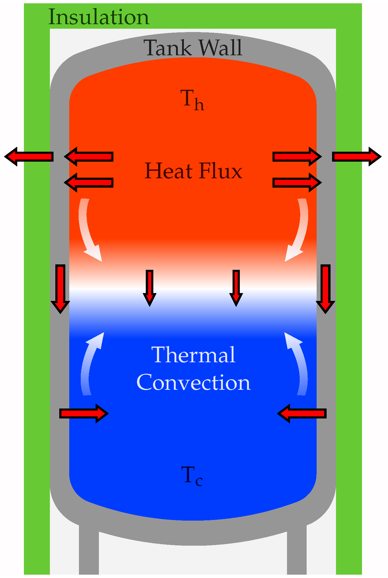
The most efficient way of using a TES as part of an energy storage system with only one storage tank is to stratify the storage fluid by its temperature-dependent density and therefore to increase the amount of exergy that can be stored [11,16]. The design of different inlet systems is a well-studied field in research to produce a high-quality stratification with a uniform hot area in the top of a tank and a denser, colder region in the bottom of the tank (see Figure 1). In between, a thermocline with a high temperature gradient and a low vertical extent should separate the two layers from each other. However, the behaviour of stratification during the stand-by period of a TES is a less investigated topic in research. In general, thermal stratification of the storage fluid is stable so that heat transfer from the hot to the cold layer can only occur due to heat conduction and not due to convection. With a thermal diffusivity of the heat transfer in water due to heat conduction is relatively slow, and thus water allows long term storage of stratified fluid layers. Nevertheless, the time in which the stratification maintains high heavily depends on the insulation of the tank and its material. Poorly insulated storage tanks lose high amounts of energy to the surroundings. However, even for well insulated tanks, where the heat loss to the environment is minimal, convection can disturb the thermal stratification. Most storage tanks are made of steel which has with a 100 times higher thermal diffusivity than water and thus the sidewalls work as a thermal bridge between the hot and the cold fluid layer. The heat flux from the hot fluid to the tank wall cools it in the near-wall regions of the upper part of the tank while the cold water in the bottom gets heated by the tank walls. Both of these processes promote thermal convection and thus reduce the level of thermal stratification. Figure 1 shows, with red arrows, a schematic depiction of the described heat fluxes within stratified TES. The white arrows indicate resulting thermal convection in the areas close to the wall.
The influence of inner lining material on the stratification in TES has only been numerically investigated by Gasque et al. [17]. They found that lining materials with low thermal conductivity potentially stabilise the thermal stratification. Nevertheless, to the knowledge of the authors, there are no experimental studies that investigate in detail the thermal convection inside stratified TES. Moreover, it is not clear what are the characteristics of the thermal convection and how exactly it reduces the degree of stratification in the TES.
Therefore, in this paper, optical measurement methods are applied on a model experiment to investigate velocity as well as temperature fields in stratified TES. In experimental fluid mechanics, particle image velocimetry (PIV) has ascended to one of the essential velocity measurement techniques since its invention [18]. This technique uses illumination equipment and cameras to track the motion of tracer particles seeded into the fluid of an experiment and thus to evaluate the velocity field of the flow. Depending on the number of used cameras and the illumination facility it is possible to measure instantaneous velocity fields with at least two velocity components in a measuring plane (2d2c) up to the entire three-dimensional velocity field of all the velocity components (3d3c). With the PIV technique, it is, possible to measure not only the velocity in one point but in thousands of position in the measurement space. Therefore, it is used in this work to measure the planar velocity field of the thermal convection perpendicular to the tank wall in a stratified TES.
Since the optical velocity measurements can only show the characteristics of the flow field in thermal convection, the knowledge of the temperature distribution in the thermal boundary layer as well as in the thermal stratification gives more profound insights and a better understanding of the processes. By replacing the standard tracer particles of a PIV setup by thermochromic liquid crystals [19] or photo-luminescent particles [20] it is possible to measure velocity and temperature simultaneously. However, due to the need of special illumination sources and cameras, these techniques are very cost-intensive and of high complexity. Therefore, in this paper, the background-oriented schlieren method (BOS) in combination with an individual evaluation algorithm, is tested to measure the temperature distribution of the thermal convection processes. During a BOS measurement, images of a textured background pattern placed behind the optically accessible experiment are taken [21]. Refractive index changes inside the experiment, for instance, due to thermal or compressible effects, lead to a seeming shift of the background on the camera images. A standard PIV software can evaluate the BOS images to calculate the refractive index gradients. With the physical dependencies between the refractive index of a fluid and its density and temperature, these quantities can be evaluated afterwards. Therefore, BOS provides the possibility of measuring different physical quantities of interest and, at the same time, being easy to implement in an already existing PIV setup.
2. Model Experiment
2.1. Description
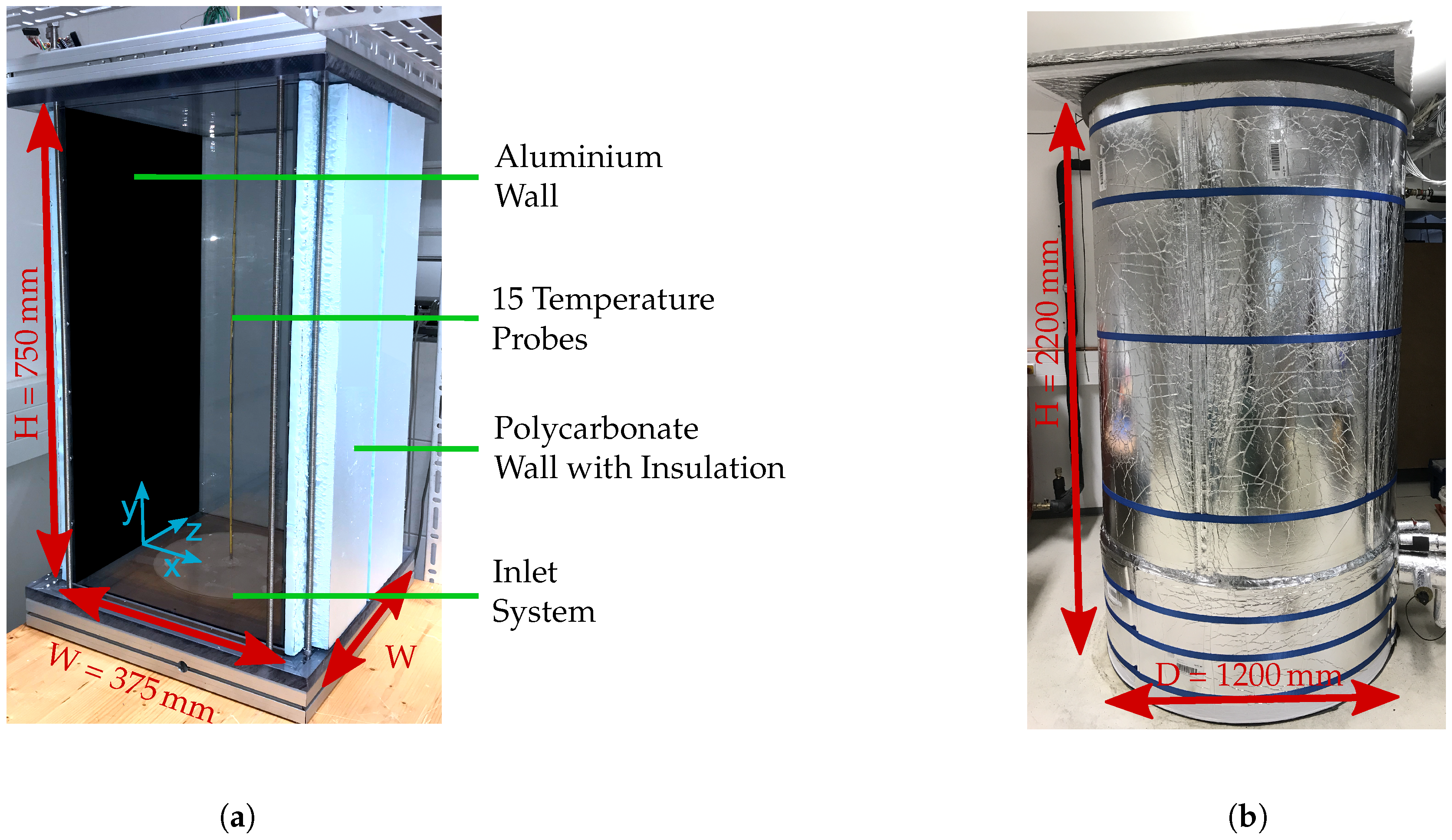
To measure the influences of thermal convection inside TES a model experiment has been built, as real storage tanks are with volumes of several cubic meters and their lack of optical access not suitable for optical measurement techniques like PIV or BOS. The model experiment of a stratified TES (hereinafter referred to as measuring cell) consists of polycarbonate sidewalls with a height on a square base of and thus has a volume of . The bottom panel of the measuring cell has a built-in inlet system consisting of an inlet port connected to a water reservoir and a circular impingement plate above. This enables a low-momentum filling of the measuring cell and thus avoids mixing of fluid layers with different temperatures. An aluminium plate with a thickness of can be placed next to a sidewall of the cell and simulates a highly thermally conductive sidewall of a storage tank. With aluminium has a two orders of magnitude higher thermal diffusivity than water so that the plate induces thermal convection near its surface as described in the previous section. Polycarbonate has been chosen as it has with nearly the same thermal diffusivity as water. Therefore, the other sidewalls cannot induce this parasitic thermal convection. The vertical temperature profile of the thermal stratification during an experiment can be measured in the water by 15 equidistantly spaced thermocouples in the vertical direction. Due to recalibration, the thermocouples achieve an accuracy of . In addition, the aluminium plate features 15 PT100 elements positioned at the same vertical distances with an accuracy of (with temperature in ). To minimise heat losses to the environment, all sidewalls and the cover panel of the measuring cell are insulated with polystyrene panels of thickness. A photograph of the described measuring cell is shown in Figure 2a.
2.2. Proof of Comparability
To proof that the model experiment mimics a real TES, a comparison of the measuring cell and a prototype steel TES with a volume of has been made. In this steel tank, ten PT100 temperature sensors with an accuracy of are installed over the height to measure the vertical temperature profile. The tank is insulated by vacuum insulation panels (VIP) [22] with an equivalent thermal conductivity in the range of several so that energy losses to the surroundings are minimised. A photograph of the real TES with vacuum insulation is shown in Figure 2b.
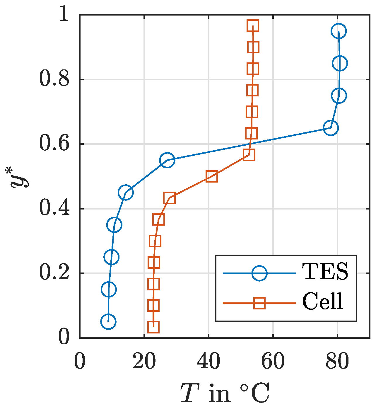
To compare the TES and the measuring cell with one another, they have been filled with thermal stratifications that are shown in Figure 3. The vertical temperature profiles with the dimensionless height are located in different temperature ranges as the possible temperature range in the measuring cell is limited in comparison to the TES where temperatures up to are possible for elevated pressures of . The thermocline of the TES is located in the region of = 0.4–0.7 while the thermocline of the measuring cell is positioned between = 0.4–0.6. This shows that the level of stratification in the measuring cell is slightly better than in the real TES due to a more gently and faster filling process.
For comparison of how intense the mixing of the temperature layers in the two different storage systems is, the energy and exergy efficiencies are evaluated. The energy efficiency shows how much losses to the surroundings occur while the exergy efficiency shows how much of the energy contained in the storage can be transformed to work and thus shows how high the degree of stratification is.
For this evaluation, both systems are virtually divided into N fluid layers with , where N is the number of temperature sensors of the corresponding system. For each of these layers the contained energy can be calculated for each time step as shown in Equation (1) and the exergy of each layer and time step can be calculated using Equation (2), respectively [16].
C and stand for the specific heat capacity of the water and the temperature of the surroundings and are assumed to be constant. represents the mass of the related fluid layer and stands for the temperature of the fluid layer at the time of t. The efficiencies of the energy and exergy content of a system are then calculated by:
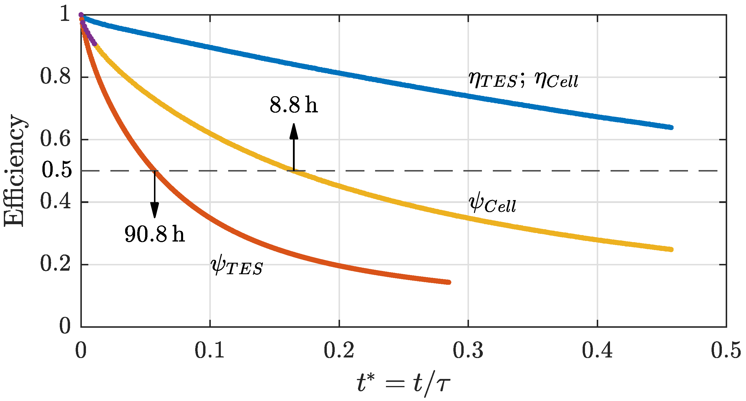
Figure 4 shows the comparison of the exergy efficiencies of the TES and the measuring cell over the dimensionless time , where is the time in which the mean dimensionless temperature of the storage fluid
drops exponentially from 1 to . stands here for the volume-averaged temperature in the tank with .
The value of depends on the quality of the insulation of a storage tank. The better the insulation, the higher the value of . The time constant of the investigated TES is while the measuring cell’s time constant is . The TES has a smaller volume to surface ratio, and the vacuum insulation of the TES has one order of magnitude lower thermal conductivity than the polystyrene insulation of the measuring cell. This results in much better insulation of the TES and therefore in its higher time constant.
Due to normalisation of the time by the individual time constants of the storage systems and plotting the energy efficiencies and over this time both have the same shape by definition which is shown by the blue line in Figure 4. If heat transfer from the hot water not to the surroundings but the cold water in the bottom layer happens, the overall energy in the storage tanks stays the same. In contrast to that, the exergy efficiency drops during this process as only temperature differences between the storage fluid and the environment can be transferred into work and this difference decreases during the temperature compensation inside the tank. Therefore, the faster the exergy efficiency of a storage tank decays in comparison to its energy efficiency, the faster the decline of the stratification level in the tank.
The comparison of the exergy efficiency of the measuring cell with that of the TES in Figure 4 shows that the exergy in the TES drops in a non-dimensionalised time scale much faster. Although the aluminium plate in the measuring cell has a temperature diffusivity seven times higher than the steel wall of the TES, the TES achieves an exergy efficiency of in a period of . In contrast, this process in the measuring cell takes a normalised time of . In real-time, these values correspond to and , respectively, as shown in Figure 4. Reasons for that are the better insulation of the TES that reduces energy losses to the environment but not the temperature compensation inside the tank, and the higher temperature difference of the TES’s thermal stratification. With this, the heat flux in the wall and the adjacent vertical convection increase, and the exergy decreases faster.
Overall, the exergy analysis has shown the negative influence of the heat transfer processes inside thermal storages on the thermal stratification. In a transient process, the efficiency of a TES reduces, as shown by the steeper drop in exergy efficiency compared to energy efficiency. Furthermore, it shows that the measuring cell as a model experiment is capable of simulating a real TES, even if the exergy losses are not identical. The larger a tank is, the higher is the possibility of turbulent vertical convection, which causes the exergetic efficiency to decrease and thus is of paramount importance for large-scale energy storage for Carnot batteries [6]. Additionally, the comparison of vertical temperature profiles of different filling processes has shown that the thermal stratification is reproducible. This allows the comparison of results of different measurements if the measuring cell is filled in the same way.
3. Methodology
3.1. Planar Particle Image Velocimetry
For measuring the two-dimensional, time-resolved motion of a fluid by PIV, the fluid is seeded with tracer particles that follow the flow faithfully. The measuring plane is illuminated most commonly by a laser which light beam gets spread to a light sheet by a cylindrical lens. The illuminated particles get captured by a camera at different time steps so that a motion of the particles between the different images is noticeable. To evaluate the velocity out of these images, they get divided into interrogation windows. Two interrogation windows which are at the same position of the field of view but from different time steps are evaluated by cross-correlation. The position of the cross-correlation’s maximum value determines the displacement of the particles in this window and defines the vector of the motion at this region. For more details of the various techniques, the interested reader is referred to Raffel et al. [23] and Adrian and Westerweel [24] and for recent developments to Kähler et al. [18].
3.2. Background-Oriented Schlieren
3.2.1. Measuring Principle
To apply the BOS measurement technique, a textured background pattern, for instance, a random dot pattern, has to be created. In measurement, the camera focuses on this background pattern that is placed behind the investigated region. The first step to measure thermal or compressible effects in this region is to take a reference image of the background pattern before there are any refractive index changes due to thermal or compressible effects present in the measuring area. After that, a series of measurement images can be taken. Thermal or compressible effects which are present in the measurement region during the exposure of the measurement images lead to apparent distortion of the background pattern compared to the reference image which relies on the intermediate changes in refractive index.
With the help of a PIV evaluation algorithm, the apparent distortion of the background pattern due to refractive index changes are evaluated by dividing the raw images into small interrogation windows and correlate the windows of the reference image with the corresponding windows of the measurement image. This process results in a high-resolution displacement matrix of the reference and the measurement image. By creating the random dot pattern that way, each dot covers about three pixels on the camera sensor, and about ten dots are within one interrogation window, the best possible results in the PIV evaluation are achieved [23].
Figure 5 shows the principle of the BOS method on the example of the measuring cell. The yellow dotted line shows the path of the light from position 1 to the camera without thermal stratification in the cell. The black line indicates the path of light with a present stratification (between the hot temperature , and the cold temperature ) and the red line shows the apparent path of the light by looking at the camera image. The displacement on the background from position 1 to position 2 can be projected in the measuring plane, which is indicated by the green arrow.
3.2.2. Evaluation of Temperature Fields from BOS Measurements
For further evaluation of the displacement fields, the method presented by Dalziel et al. [25,26] is applied to obtain the gradient of the density from the displacement matrix. The displacements in the x-direction and in y-direction obtained by the PIV algorithm are directly proportional to the gradients of the changes in the refractive index:
are the width of the cell, the distance to the background and the thickness of the sidewalls from the experiment as shown in Figure 5 and are the refractive indices of water at the temperature of the reference image, of the air around the experiment and of the polycarbonate sidewalls. By using the already mentioned geometric parameters together with the distance L, between the camera sensor and the background pattern, and the mentioned refractive indices, the magnification factor M is calculated to convert the apparent displacements from the background to the mid-plane of the cell [25]:
With the temperature-independent and constant relationship between the density and the refractive index n of a fluid:
where is the density in the reference condition, Equations (6) and (7) can be written as:
By numerical integration of Equations (10) and (11) the density changes within the field of view can be determined. The value at the starting point of the integration of equals zero. For obtaining the absolute density field, it is necessary to know the absolute density at least at one position in the field of view and to use this position as the starting point for the integration so that the density from this position can be added as a constant offset. Finally, with the resulting density field and the known non-linear dependence between temperature and density of water, the temperature field can be calculated. Due to this non-linear dependence, the direct calculation of the temperature from the refractive index gradient is not possible, and a stepwise evaluation via the density is necessary.
4. Experimental Setups
4.1. PIV Setup and Measuring Procedure
For the characterisation of thermal convection and its influences on the thermal stratification, PIV measurements are applied to measure the velocity field. As the vertical, thermal convection is only present in the wall adjacent regions of the measuring cell and the flow is dependent of the height, the measurements are carried out only near to the aluminium wall with a relatively small field of view and in three different heights. Thus it is possible to resolve the velocity boundary layer of the vertical convection, to characterise the flow pattern and to measure the maximum vertical and horizontal velocities in the different regions.
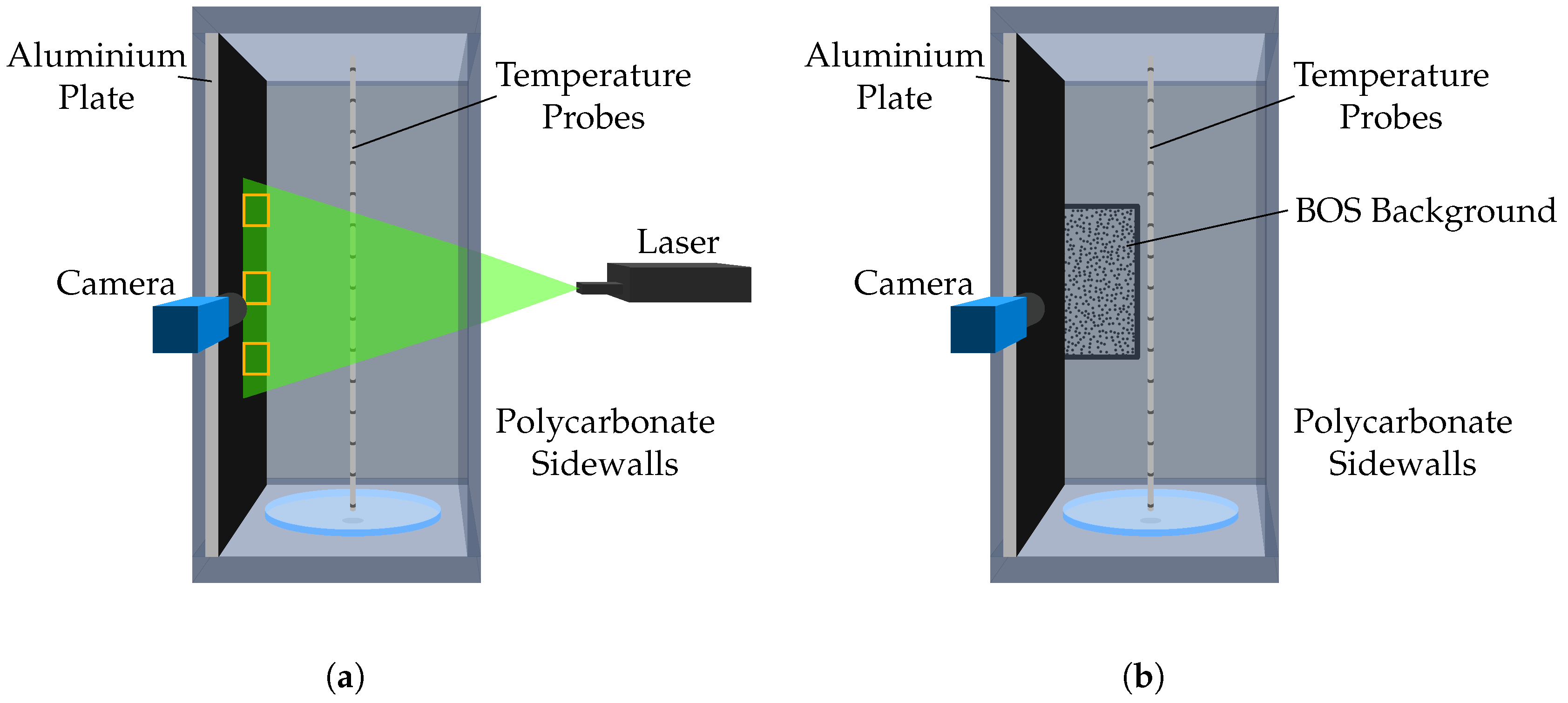
Figure 6a shows a schematic of the PIV setup. The light sheet is oriented perpendicular to the wall within the xy-plane. Orange rectangles indicate the different measurement positions in the hot part of the thermal stratification, on half of the cell height within the thermocline and the in the lower, cold part of the stratification.
The laser and the camera are arranged at an angle of , as shown in Figure 6a. The sCMOS camera (Imager LaVision GmbH) has a sensor size of with a pixel size of . The objective lens (Zeiss Milvus 2/100M) has a focal length of and a minimal f-number of . The obtained field of view has a size of about with a resolution of . For the illumination, a Nd:YAG double-pulse laser (Continuum Minilite by ILA GmbH) with a wavelength of and a pulse energy of is used to form the light sheet. The time between the double pulses may vary from up to at repetition rates from to .
The used particles with a diameter of are made of polyamide and have a density of . They have been chosen as their velocity due to sedimentation has been calculated to be (at water temperature) [23], where is the particle’s diameter, the particle’s and the fluid’s density, is the dynamic viscosity and g the acceleration due to gravitation. Therefore, the sedimentation velocity of the particles is much lower than the expected flow velocity of the thermal convection, which, according to preliminary investigations, is in the order of .
For the calibration, a commercial calibration target with a size of is placed in the corresponding measurement position. Then the measuring cell gets filled with a thermal stratification. Therefore, a reservoir of water is placed next to the experiment, where the water can be cooled down to a minimum temperature of before starting a filling process. During the filling process, the water gets heated by a flow heater which is capable of heating the water to a maximum temperature of . When half of the cell volume is filled with hot water, the second half is filled through a by-pass so that this water is not heated. As the hot water heats the measuring cell during the filling process and the cold water cools it down again, the resulting maximum temperature difference in the measuring cell is about . After the end of the filling process, the calibration is performed. The procedure for the measurement after the calibration is the same.
4.2. BOS Setup
The BOS setup is similar to the PIV setup shown in Figure 6b. The laser is replaced by a BOS background pattern placed behind the cell in the height of the measurement position. The pattern is a generated random-dot pattern with a dot diameter of and a dot density of per . The pattern is printed with black colour on white paper which is illuminated from behind during a measurement with a LED spotlight. Although the points on the background have no gradation in their grey levels, their darkest area on the resulting camera image is in the middle with slightly brighter pixels around. This gradation in brightness allows a cross-correlation peak detection in the subpixel range due to a Gaussian peak fit that is implemented in the PIV algorithm.
The LED illumination has been chosen as its thermal radiation is much lower compared to a halogen spotlight and thus minimises the temperature input to the experiment. Additionally, the power input of is relatively high for LED illuminations which leads to high luminous intensity on the background and thus to a high signal to noise ratio on the camera image.
For performing a measurement, the measuring cell gets filled in the same way as described in the section before. But instead of performing a calibration previously, it is necessary to make a reference image for the BOS measurement. Therefore, the measuring cell and the water in the reservoir are left to stand until both of them reach room temperature. Then the measuring cell gets filled with the water without heating. Due to the same temperatures of water and measuring cell, no thermal convection is present inside the experiment. In this state, the reference image can be taken and afterwards, the cell can get filled with stratification, and the measurement can be carried out.
5. Results and Discussion
With the described setups and the corresponding measuring procedures, both PIV and BOS measurements have been carried out. The results of the PIV velocity measurements in the different measurement positions, shown in Figure 6a, are presented and discussed in the following. Afterwards, the results of the test measurements for temperature field determination with the BOS method are presented.
5.1. PIV Velocity Measurements
Figure 7 shows the resulting velocity fields of the PIV measurements with the flow in the cold layer of the stratification (Figure 7a), in the height of the thermocline (Figure 7b) and in the hot layer (Figure 7c) [27]. The surface of the aluminium wall is at the position with . The vector arrows show the flow field with a contour plot of the vertical velocity component in the background. The cell has been filled separately for each flow field, and PIV measurements have been started five minutes after the end of filling. Preliminary, qualitative investigations have shown that this time is sufficient to allow the inlet flow in the bottom to settle down and that, at the same time, it is short enough that the high degree of thermal stratification from the beginning of the stand-by period to be still present.
Inlet temperatures of each measurement have been in a range from 58 to for hot layers and between 6 and for cold layers. The water temperatures measured inside the cell have been between 52 and in the hot layer and 9 and in the cold layer for all measurements. Changes in water temperature during the filling have occurred as the cell has to adopt the temperature of the water. Thus, the cell heats or cools the water, respectively. Differences in the measured stratification temperatures may result from different room temperatures as the measurements have not been performed at the same day. However, the typical flow features and characteristic curves that this study deals with are not significantly affected by small temperature differences between the measurements.
The evaluation of the flow fields in Figure 7a,b have been made by averaging 499 vector fields of 500 raw images with a time difference of resulting in an overall time average of . The resolution of the calculated vectors is which converts together with an overlap of 50% of the vectors to . Figure 7c shows an averaged vector field of 9000 images with the same difference in time of . The higher number of images used for the averaging is a result of fluctuations that have occurred in this region so that more time steps have been needed. As mentioned in the discussion of Figure 4, the whole process is transient. Therefore, the state of the experiment at the beginning of the measurement time is another than in the end. However, the violet part of the cell’s exergy efficiency curve shows that during the measurement time, the exergy efficiency decreases about only 10%. With the objective of this measurement to get a general impression of the flow, this change is small enough not to affect the result.
The basis of the averaging in Figure 7c are vector fields that have been calculated using the pyramid sum of correlation algorithm with Gaussian weighting [28]. This algorithm uses the correlation of not only two consecutive raw images but takes correlations of every possible combination of a range of three or more images into consideration. Therefore, low, as well as high velocities, can be evaluated at the same time, and velocity gradients can be resolved better by the cost of temporal resolution. In this case, a range of five raw images has been used to calculate one quasi-instantaneous flow field. Therefore the time averaging for one single vector field was . The spatial resolution can be increased [29], resulting in a resolution of one vector of which corresponds, with an overlap of 50% of each vector, to .
The time-averaged flow fields show two vertical wall jets, one in the hot and one in the cold layer of the stratification. The downward-directed jet in the upper part results from the heat flux that heats the aluminium wall and cools the water in this region and the upward-directed jet in the lower part is a result of the cold water which gets heated by the aluminium wall in this region. The two counter-directed wall jets approach at in the region of the thermocline which can be seen in Figure 7b. The collision slows down the wall jets and creates a relatively weak horizontal flow towards the centre of the measuring cell. The horizontal velocities of this flow are one to two orders of magnitude lower than the vertical velocities in the wall jets at this height as the flow spreads over a broader region as in the wall jets.
Comparison of Figure 7b with Figure 7a,c shows that the velocities of the wall jets increases with greater distance to the centre of the thermocline. The maximum of their thickness does not seem to be reached in the regions shown since both jets widen continuously in the areas of the Figure 7b,c. Further comparison of the two wall jets with one another shows that the upward-directed jet is thicker but slower than the downward-directed jet. This behaviour is plausible taking into account the kinematic viscosity of water which differs from for the cold temperature of and for the hot temperature of resulting in a change of 57% [30]. The higher viscosity in the cold layer leads to a thicker wall jet because of the higher friction in the fluid. Furthermore, the lower viscosity in the upper part favours higher velocities and a thinner wall jet at the same time. As indicated earlier, there are more fluctuations in the velocity field in the upper part, which made averaging over more individual time steps necessary to obtain the velocity field in Figure 7c. These fluctuations are investigated in more detail in the following.
For this reason, time-series data of the vertical velocity component as well as its normalised temporal development has been analysed at three points in space where each of them is in the middle of one of the investigated three measurement areas. The results are shown in Figure 8. The vertical positions of the three points are as shown in the legend of diagram Figure 8a. The horizontal positions of the points have been chosen to be away from the wall surface which equals as this is still inside the field of view but at the same time outside of the wall jets of the time-averaged flow fields. In this position, the velocity should be steady and near to zero in the case of laminar flow. Otherwise, fluctuations occur that can be analysed to get a deeper understanding of the flow characteristics.
Figure 8a shows that the flow in the bottom at and in the thermocline at seems to be laminar because both of the time-series stay nearly constant over the entire period of . In the cold region at a height of the measured vertical velocity is with an averaged value of negative compared to that in the thermocline at with . The negative velocity shows that outside of the wall jet, a counter-directed shear flow is existent, which can be explained by the inertia of the fluid. A small fluid portion that flows with the wall jet upwards indeed reaches the height where it has the same density as stratification in this height, but due to its inertia, it is flowing beyond this position. Therefore, the buoyancy force acting on the fluid portion changes its sign so that the fluid has to flow back, which results in the shear flow. In the thermocline, both wall jets approach and thus a shear flow is not existent in this area.
The vertical velocity component in the hot part of the stratification shows a completely different behaviour than in the other parts of the cell. It constantly changes and thereby varies between a minimum velocity of to a maximum of . The difference between the velocities in the hot and cold layer is due to the temperature dependant properties of water, as stated before.
Figure 8b shows the same time-series as before but normalised by their maximum values. It is noticeable that the relative fluctuations in the thermocline are nearly as high as in the hot region shown in their standard deviations of and , respectively. In comparison to that, the normalised velocity in the bottom region of the measuring cell is still nearly constant with a standard deviation of only . In contrast to the signal of the hot part, the velocities in the thermocline and the bottom are much more covered by noise. This is since the relative uncertainty of PIV measurements is higher for lower velocities as the particle shift between the images is shorter while the accuracy of the position determination remains the same with about [23]. Most of the fluctuations in the bottom region can be attributed to this noise. In contrast, the velocity in the thermocline undergoes, additionally to the noise, significant changes that cannot be seen in Figure 8a. As a result, the normalised time-series of the velocity shows that the fluctuations, which emerge in the wall jet of the hot layer, spread to the thermocline. There, they seem to decay as their influence is not noticeable in the cold part of the stratification.
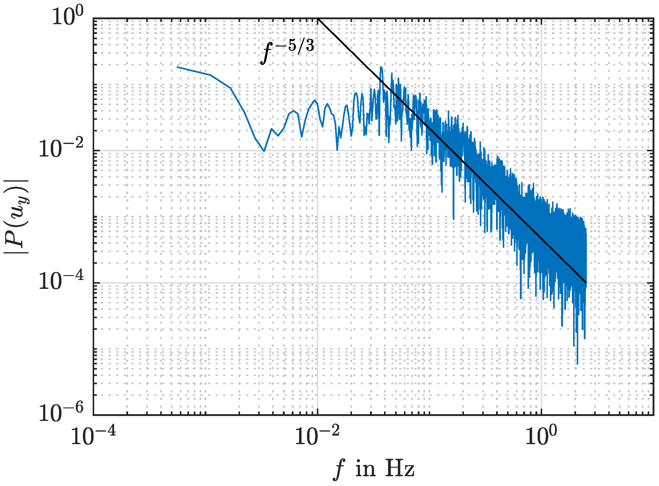
As a last step the amplitude spectrum of the vertical velocity at has been calculated, to check whether there is any kind of periodicity in the flow. For this reason, the whole data set of 9000 raw images has been used, corresponding to a period of 1800 s. Significant periodic features of the flow would result in an outstanding peak of the spectrum. Figure 9 shows the results of the amplitude spectrum in a logarithmic scale. Starting at the lowest frequency the spectrum stays nearly constant with values in the range of , and starts to decay with a nearly linear slope (in the logarithmic scale) from a frequency of about . During this decay no significant peak in the spectrum can be recognised and therefore the flow in this region seems not to have a dominant periodic frequency. However, the spectrum is during its decrease parallel to , and thus it follows the typical behaviour of turbulent motion described by Kolomogorovs -law. The law describes the fact that large vortices in turbulent motion disintegrate into smaller ones until their kinetic energy transfers into heat due to viscosity. In future investigations the vortices in the fluctuating flow in the upper part of the cell will be investigated more precisely. Furthermore, it can be assumed that the flow is not only two-dimensional but has a third component, which can be measured in the future by stereoscopic or tomographic PIV investigations.
5.2. Temperature Field Measurements with the BOS Method
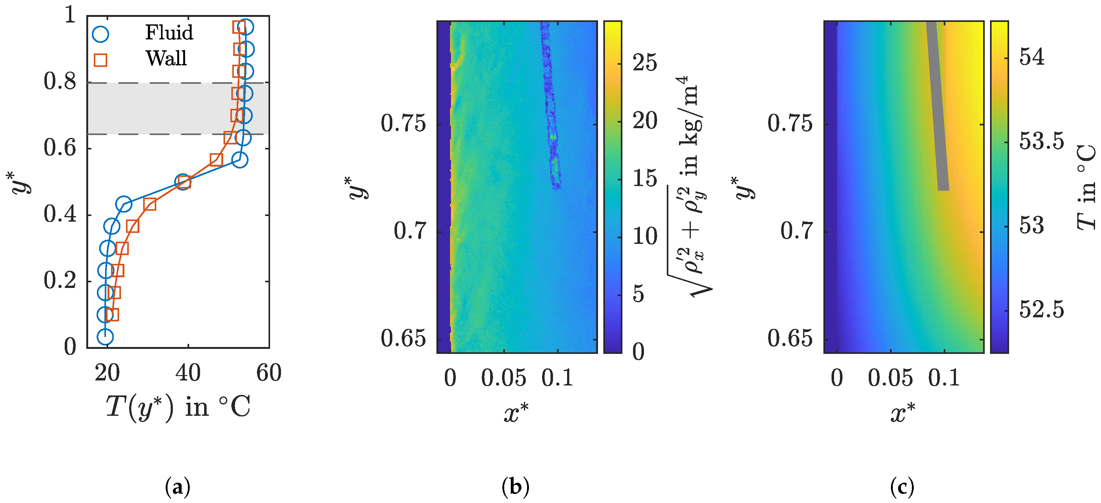
To test the measuring principle and the evaluation procedure of the BOS method described in the previous section, measurements in the region of the convective wall jet shown by the velocity measurements have been done. Therefore, the measuring cell has been filled with a stratification shown in Figure 10a by vertical temperature profiles measured in the fluid and the aluminium wall, respectively. The dashed lines indicate the height the measurement has been taken and show that the entire field of view lies in the hot layer of the stratification, but also not far above the thermocline. Therefore, the temperature of the aluminium wall in the lower part of the field of view already decreases. The temperature of the water in this region is nearly the same as in the whole field of view. In comparison to the PIV measurements, the field of view has become larger as the distance between the camera and measuring cell has been adjusted to focus on the background picture.
Figure 10b,c show instantaneous snapshots of the magnitude of the density gradient and the resulting temperature field five minutes after filling the measuring cell. To calculate those, the raw images of the measurements have been evaluated by the PIV algorithm with a size of the interrogation window of and an overlap of 50% which results in a spatial resolution of the camera in the mid-plane of the measuring cell of and a region of that is represented by one displacement vector. Before calculating the density gradients from the displacement vector field, a median filter has been applied that removes vectors which are more than two times bigger than the median of their neighbours in a region of vectors and replaces them with the median vector [31]. This step has been applied as all incorrectly evaluated values get summed during the integration of the density gradient.
To be able to calculate the absolute density, as discussed in the previous section, additional temperature sensors have been installed in the measuring cell. One sensor was positioned in a distance of to the wall surface and can be seen on the upper right side of Figure 10b. The bottom part of this sensor has been chosen to be the starting point of the integration of the density gradients as the density in this position can be found by the measured temperature. The area of the sensor is masked in grey in the temperature field of Figure 10c to indicate this starting point, and since the evaluation of the temperature in this area is influenced by the sensor. Another temperature sensor has been glued on the wall surface at the height of to work as a verification spot for the finally evaluated temperature field. Due to its small size, it cannot be seen in the evaluated images.
The magnitude of the density gradient field shows the highest density gradient on the left side attached to the surface of the aluminium wall (at ) with up to . With increasing distance to the wall surface, the density gradient decreases until it reaches its minimum value on the upper right part of the field of view with . A more precise look to the area with the high gradients shows that their decay from the left to the right side of the field of view is not steady as the gradients change between lower and higher values.
A high density gradient shows—even if it is not directly proportional—a region of a high temperature gradient. Therefore, the structures on the left side of the figure which are attached to the wall indicate local temperature differences. The temperature boundary layer of laminar, vertical convection would rise steadily from a lower temperature at the wall surface to a higher temperature in the bulk region of the measuring cell. Thus, the density gradient field of laminar vertical convection should be a steady decrease, which leads here to the result that the examined structures are a consequence of the turbulent velocity fluctuations that have been described in the discussion of the PIV measurements.
By looking at the temperature field in Figure 10c these small structures cannot be seen as a local difference in temperature which shows that these differences are small compared to the temperature differences in the boundary layer. Nevertheless, the temperature boundary layer of the vertical convection is visible with low temperatures on the left side adjacent to the wall and high temperatures on the right side. These high temperatures increase in the upper right corner up to , and they are thereby in a similar range as the temperature of the sensor in the middle of the cell. The thickness of the temperature boundary layer increases in the bottom part of the temperature field. The observation of the verticle temperature profiles in Figure 10a shows that the temperature difference between water and wall in the lower part of the field of view gets higher. Thus, the heat flux from the water to the wall is higher in this region, which results in the thicker temperature boundary layer.
For verification, the BOS results are compared to the measured temperature of the sensor glued on the wall surface. At the time of the shown temperature field, the sensor has measured a temperature of . This value is equal (with respect to the uncertainty of ) to the temperature evaluated by the BOS measurement at this position. As a result, this shows that the BOS method is capable of measuring high-resolution temperature fields in transparent media.
Since not only one measurement image, but a short series of 200 images ( at sampling frequency) has been taken, the BOS method can be used to analyse the temporal development of the temperature. However, in this case, time-series data of the temperature at various locations in the field of view have not shown significant changes in temperature and are therefore not presented here. But in general, the long-term development of temperature can be studied with this method. It can also be used in experiments with higher temperature variations since the temporal limitation is the same is for single frame PIV measurements and is therefore only limited by the used camera.
Certainly, it is to mention that temperature measurements with the BOS method are subject to some restrictions which are to be considered before applying the technique. Gradients of the refractive index which occur parallel to the viewing direction of the camera (at small angles of the aperture of the camera this corresponds here to the z-axis in good approximation), do not lead to a distortion of the background and therefore cannot be measured. Besides, all gradients of the refractive index that occur in the x- or y-direction are summed over the entire depth of the measuring cell in the z-direction.
In the presented case, the influences of these restrictions are relatively small. Due to the stable thermal stratification of the water and the camera’s viewing direction parallel to the wall, strong density gradients do not occur in the viewing direction. Thus, the technique is capable of evaluating most of the occurring changes in refractive index, and therefore the resulting temperature distribution should be in good agreement to the real temperature field in the measurement plane.
In contrast, when interpreting the structures in the density gradient field, care must be taken to ensure that they are integrated over the entire depth of the cell. This leads to the problem that an observed structure cannot be matched to a particular position in the z-direction. One possibility to solve this issue would be to perform simultaneous PIV and BOS measurements and to correlate time-series data of the density gradients and the velocity. Structures in the density gradient field that do not correlate with the velocity would then have to be in another z-position.
6. Conclusions
The study presents velocity as well as temperature measurements on an experiment that is used to characterise the influence of thermal convection inside thermal energy storages (TES) with thermally stratified storage fluid. A model experiment has been built, and for comparison with a real TES, an exergy analysis has been carried out which has shown that the model is capable of simulating a real storage tank.
Planar PIV velocity measurements in the mid-plane of the measuring cell have been performed to investigate the flow phenomena that result from a heat flux through a simulated tank wall when a thermal stratification of the working fluid is present in the measuring cell. By using the pyramid correlation approach a spatial resolution of could be reached. With the high-resolution measurements, for the first time two counter-directed, vertical wall jets have been observed in time-averaged vertical velocity fields, that are adjacent to the wall. One of the jets emerges in the upper, hot part of the stratification as a result of heat flux from the working fluid to the sidewall and thus the jet flows downwards. The second jet develops due to a heat flux that comes from the wall and heats the cold fluid resulting in an upwards rising wall jet. In the thermocline, both jets get slowed down, approach each other and disappear in a slow wide-spreading horizontal flow. Time-series data near the upper wall jet, in the thermocline and adjacent to the lower wall jet, have shown that the flow in the hot layer underlies strong fluctuations that reach to the thermocline but are not present in the cold layer any more.
For more insight into the flow, the background-oriented schlieren method (BOS) has been applied to perform temperature field measurements in the thermal boundary layer of the vertical flow. The spatial resolution has been in the x and y-directions, respectively. It has been shown that the BOS method can be used as long as there are no changes in the refractive index of the working fluid in the viewing direction of the camera as every measurable change in this direction gets integrated over the depth direction. Test measurements with the BOS setup have been evaluated to obtain a field of the density gradients’ magnitude and the temperature field. Spatial structures that are in good agreement with the results of the velocity measurements have been detected in the density gradient field, and the temperature field has shown the thermal boundary layer of the natural convective flow. Additionally, the evaluated temperatures have been verified by the measured temperature of a sensor within the field of view.
In the future, further velocity measurements using multiple cameras to observe the flow in different regions simultaneously will be carried out based on this study. With the help of the BOS method, it is possible to observe fluctuations in the density or temperature field parallel to the velocity measurements. Furthermore, due to the knowledge of the density gradient field, phenomena like gravitational waves can be investigated. To compare the results from the measuring cell with large storage tanks, the influences of various parameters such as the temperature difference of the stratification or the wall material will be analysed and characteristic dimensionless numbers will be determined.
Author Contributions
Conceptualisation, C.R., C.C. and H.O.; methodology, C.R., C.C. and H.O.; software, H.O.; formal analysis, H.O.; investigation, H.O.; resources, C.C.; data curation, H.O.; writing—original draft preparation, H.O.; writing—review and editing, C.R. and C.C.; visualisation, H.O.; supervision, C.R. and C.C. All authors have read and agreed to the published version of the manuscript.
Funding
This research was partly funded by the European Regional Development Fund (ERDF) in cooperation with the Thüringer Aufbaubank (2017 FE 9086).
Acknowledgments
The authors thank Alexander Thieme and Clemens Naumann for their help in setting up the experiment and supporting the measurements and Jens Christian Fokken for the implementation of the BOS technique during his master thesis.
Conflicts of Interest
The authors declare no conflict of interest.
Abbreviations
The following abbreviations are used in this manuscript:
| BOS | background-oriented schlieren |
| LED | light-emitting diode |
| PIV | particle image velocimetry |
| TES | thermal energy storage |
| VIP | vacuum insulation panel |
References
- Gielen, D.; Boshell, F.; Saygin, D.; Bazilian, M.D.; Wagner, N.; Gorini, R. The Role of Renewable Energy in the Global Energy Transformation. Energy Strategy Rev. 2019, 24, 38–50. [Google Scholar] [CrossRef]
- Laughlin, R.B. Pumped Thermal Grid Storage with Heat Exchange. J. Renew. Sustain. Energy 2017, 9, 044103. [Google Scholar] [CrossRef] [Green Version]
- Cao, K.K.; Nitto, A.N.; Sperber, E.; Thess, A. Expanding the Horizons of Power-to-Heat: Cost Assessment for New Space Heating Concepts with Wind Powered Thermal Energy Systems. Energy 2018, 164, 925–936. [Google Scholar] [CrossRef]
- Thess, A. Thermodynamic Efficiency of Pumped Heat Electricity Storage. Phys. Rev. Lett. 2013, 111, 110602. [Google Scholar] [CrossRef] [PubMed] [Green Version]
- Gur, I.; Sawyer, K.; Prasher, R. Searching for a Better Thermal Battery. Science 2012, 335, 1454–1455. [Google Scholar] [CrossRef] [PubMed]
- Steinmann, W.D.; Jockenhöfer, H.; Bauer, D. Thermodynamic Analysis of High-Temperature Carnot Battery Concepts. Energy Technol. 2020, 8, 1900895. [Google Scholar] [CrossRef] [Green Version]
- Thess, A.; Trieb, F.; Wörner, A.; Zunft, S. Herausforderung Wärmespeicher. Phys. J. 2015, 14, 33–39. [Google Scholar]
- Pelay, U.; Luo, L.; Fan, Y.; Stitou, D.; Rood, M. Thermal Energy Storage Systems for Concentrated Solar Power Plants. Renew. Sustain. Energy Rev. 2017, 79, 82–100. [Google Scholar] [CrossRef]
- Zanganeh, G.; Pedretti, A.; Zavattoni, S.; Barbato, M.; Steinfeld, A. Packed-Bed Thermal Storage for Concentrated Solar Power—Pilot-Scale Demonstration and Industrial-Scale Design. Sol. Energy 2012, 86, 3084–3098. [Google Scholar] [CrossRef]
- Arteconi, A.; Hewitt, N.; Polonara, F. Domestic Demand-Side Management (DSM): Role of Heat Pumps and Thermal Energy Storage (TES) Systems. Appl. Therm. Eng. 2013, 51, 155–165. [Google Scholar] [CrossRef]
- Cabeza, L.F. Advances in Thermal Energy Storage Systems; Woodhead Publishing: Cambridge, UK, 2015. [Google Scholar]
- Hedegaard, K.; Mathiesen, B.V.; Lund, H.; Heiselberg, P. Wind Power Integration Using Individual Heat Pumps—Analysis of Different Heat Storage Options. Energy 2012, 47, 284–293. [Google Scholar] [CrossRef]
- Okazaki, T. Electric Thermal Energy Storage and Advantage of Rotating Heater Having Synchronous Inertia. Renew. Energy 2020, 151, 563–574. [Google Scholar] [CrossRef]
- Okazaki, T.; Shirai, Y.; Nakamura, T. Concept Study of Wind Power Utilizing Direct Thermal Energy Conversion and Thermal Energy Storage. Renew. Energy 2015, 83, 332–338. [Google Scholar] [CrossRef] [Green Version]
- Howes, J. Concept and Development of a Pumped Heat Electricity Storage Device. Proc. IEEE 2012, 100, 493–503. [Google Scholar] [CrossRef]
- Dincer, I.; Rosen, M. Thermal Energy Storage: Systems and Applications, 2nd ed.; Wiley: New York, NY, USA, 2011. [Google Scholar]
- Gasque, M.; González-Altozano, P.; Maurer, D.; Moncho-Esteve, I.J.; Gutiérrez-Colomer, R.P.; Palau-Salvador, G.; García-Marí, E. Study of the Influence of Inner Lining Material on Thermal Stratification in a Hot Water Storage Tank. Appl. Therm. Eng. 2015, 75, 344–356. [Google Scholar] [CrossRef]
- Kähler, C.J.; Astarita, T.; Vlachos, P.P.; Sakakibara, J.; Hain, R.; Discetti, S.; La Foy, R.; Cierpka, C. Main Results of the 4th International PIV Challenge. Exp. Fluids 2016, 57, 97. [Google Scholar] [CrossRef] [Green Version]
- Moller, S.; König, J.; Resagk, C.; Cierpka, C. Influence of the Illumination Spectrum and Observation Angle on Temperature Measurements Using Thermochromic Liquid Crystals. Meas. Sci. Technol. 2019, 30, 084006. [Google Scholar] [CrossRef]
- Massing, J.; Kähler, C.J.; Cierpka, C. A Volumetric Temperature and Velocity Measurement Technique for Microfluidics Based on Luminescence Lifetime Imaging. Exp. Fluids 2018, 59, 163. [Google Scholar] [CrossRef]
- Raffel, M. Background-Oriented Schlieren (BOS) Techniques. Exp. Fluids 2015, 56, 60. [Google Scholar] [CrossRef] [Green Version]
- Otto, H.; Müller, A.; Wollheim, T.; Thielicke, J.; Resagk, C.; Cierpka, C. Vakuum-Isolations-Paneele Für Hochleistungswärmespeicher Bis 140 °C; Thüringer Werkstofftag: Berlin, Germany, 2020. [Google Scholar]
- Raffel, M.; Willert, C.E.; Scarano, F.; Kähler, C.J.; Wereley, S.T.; Kompenhans, J. Particle Image Velocimetry, 3rd ed.; Springer: Berlin/Heidelberg, Germany; New York, NY, USA, 2018. [Google Scholar]
- Adrian, R.J.; Westerweel, J. Particle Image Velocimetry; Cambridge Aerospace Series; Cambridge University Press: Cambridge, UK, 2011. [Google Scholar]
- Dalziel, S.B.; Carr, M.; Sveen, J.K.; Davies, P.A. Simultaneous Synthetic Schlieren and PIV Measurements for Internal Solitary Waves. Meas. Sci. Technol. 2007, 18, 533–547. [Google Scholar] [CrossRef]
- Dalziel, S.B.; Hughes, G.O.; Sutherland, B.R. Whole-Field Density Measurements by ‘Synthetic Schlieren’. Exp. Fluids 2000, 28, 322–335. [Google Scholar] [CrossRef]
- Otto, H.; Resagk, C.; Cierpka, C. Convective Near-Wall Flow in Thermally Stratified Hot Water Storage Tanks. In Proceedings of the 13th International Symposium on Particle Image Velocimetry, Munich, Germany, 22–24 July 2019. [Google Scholar]
- Sciacchitano, A.; Scarano, F.; Wieneke, B. Multi-Frame Pyramid Correlation for Time-Resolved PIV. Exp. Fluids 2012, 53, 1087–1105. [Google Scholar] [CrossRef] [Green Version]
- Kähler, C.J.; Scharnowski, S.; Cierpka, C. On the Resolution Limit of Digital Particle Image Velocimetry. Exp. Fluids 2012, 52, 1629–1639. [Google Scholar] [CrossRef] [Green Version]
- Haynes, W.M. CRC Handbook of Chemistry and Physics, 96th ed.; 100 Key Points; CRC Press: Boca Raton, FL, USA, 2015. [Google Scholar]
- Westerweel, J.; Scarano, F. Universal Outlier Detection for PIV Data. Exp. Fluids 2005, 39, 1096–1100. [Google Scholar] [CrossRef]
Figure 1.
Schematic depiction of heat transfer processes in TES (red arrows) and their resulting thermal convection (white arrows). The heat flux in the tank wall is due to thermal stratification of the storage fluid between the hot temperature in the upper half of the tank and the cold temperature in the bottom.

Figure 2.
(a) Photograph of the cell used for optical measurements with height H and a square base of W × W. The coordinate system shows the origin of the measurement plane for the 2d velocity and temperature measurements. (b) Photograph of a prototype TES with a steel tank and insulated by VIP with height H and diameter D.

Figure 3.
Vertical temperature profiles of the TES and the measuring cell at the beginning of the stand-by period. indicates the dimensionless heights where H is the height of the TES and the measuring cell, respectively.
Figure 3.
Vertical temperature profiles of the TES and the measuring cell at the beginning of the stand-by period. indicates the dimensionless heights where H is the height of the TES and the measuring cell, respectively.

Figure 4.
Energy and exergy efficiencies of the measuring cell in comparison with a real TES. The time is normalised by the time constant where the time constant of the TES is and of the measuring cell , respectively. The time in which the exergy efficiencies reduce by half is indicated with arrows, and the first of the measuring cell’s exergy efficiency is marked in violet colour as this shows the period of the later shown velocity measurement.

Figure 5.
Schematic depiction of the measuring principle of BOS using the example of the thermally stratified measuring cell following Dalziel et al. [25].
Figure 5.
Schematic depiction of the measuring principle of BOS using the example of the thermally stratified measuring cell following Dalziel et al. [25].

Figure 6.
(a) Measuring setup for 2d PIV measurements in the measuring cell. Orange rectangles illustrate the size and position of the performed measurements. (b) Depiction of the BOS measuring setup in the measuring cell.
Figure 6.
(a) Measuring setup for 2d PIV measurements in the measuring cell. Orange rectangles illustrate the size and position of the performed measurements. (b) Depiction of the BOS measuring setup in the measuring cell.

Figure 7.
Averaged PIV measurements near the aluminium wall of the measuring cell. For each measurement position a separate filling was made. Every measurement started five minutes after finishing the filling to allow the flow due to the filling process to decay. (a) Upward-directed wall jet in the cold region of the thermal stratification. (b) Approaching counter-directed, vertical wall jets in the region of the thermocline. (c) Downward-directed wall jet in the hot layer. Vector arrows show the flow direction and the contour plot shows the value of the vertical component of the velocity.

Figure 8.
(a) Velocity time-series data of the PIV measurements at three different heights of the cell. The x-position of each time-series is and thus away from the wall surface. (b) Normalised time-series data of (a) by dividing the velocities by the maximum of their absolute values.
Figure 8.
(a) Velocity time-series data of the PIV measurements at three different heights of the cell. The x-position of each time-series is and thus away from the wall surface. (b) Normalised time-series data of (a) by dividing the velocities by the maximum of their absolute values.

Figure 9.
Power spectrum of the time-series of the vertical velocity over at the height . The black line indicates the exponential decrease of the function .
Figure 9.
Power spectrum of the time-series of the vertical velocity over at the height . The black line indicates the exponential decrease of the function .

Figure 10.
(a) Vertical temperature profile of the fluid in the cell and the aluminium wall at the time of the here discussed evaluations of the BOS measurement. The grey area between the dashed lines indicates the region of the measurement. (b) Instantaneous depiction of the magnitude of the local density gradients evaluated from the displacement field of the BOS measurement. (c) Temperature field resulting from the integration of the density gradients and the conversion of the density field. The region of the temperature sensor is masked in grey.

© 2020 by the authors. Licensee MDPI, Basel, Switzerland. This article is an open access article distributed under the terms and conditions of the Creative Commons Attribution (CC BY) license (http://creativecommons.org/licenses/by/4.0/).
Share and Cite
MDPI and ACS Style
Otto, H.; Resagk, C.; Cierpka, C. Optical Measurements on Thermal Convection Processes inside Thermal Energy Storages during Stand-By Periods. Optics 2020, 1, 155-172. https://0-doi-org.brum.beds.ac.uk/10.3390/opt1010011
AMA Style
Otto H, Resagk C, Cierpka C. Optical Measurements on Thermal Convection Processes inside Thermal Energy Storages during Stand-By Periods. Optics. 2020; 1(1):155-172. https://0-doi-org.brum.beds.ac.uk/10.3390/opt1010011
Chicago/Turabian StyleOtto, Henning, Christian Resagk, and Christian Cierpka. 2020. "Optical Measurements on Thermal Convection Processes inside Thermal Energy Storages during Stand-By Periods" Optics 1, no. 1: 155-172. https://0-doi-org.brum.beds.ac.uk/10.3390/opt1010011