Micro- and Macro-Scale Measurement of Flow Velocity in Porous Media: A Shadow Imaging Approach for 2D and 3D


Optical Diagnostics Lab, Department of Mechanical Engineering, University of Alberta, Edmonton, AB T6G 1H9, Canada
*
Author to whom correspondence should be addressed.
†
Equal contribution.
Optics 2020, 1(1), 71-87; https://0-doi-org.brum.beds.ac.uk/10.3390/opt1010006
Submission received: 31 December 2019
/
Revised: 5 February 2020
/
Accepted: 19 February 2020
/
Published: 25 February 2020
(This article belongs to the Special Issue Optical Diagnostics in Engineering)
Abstract
:Flow measurement in porous media is a challenging subject, especially when it comes to performing a three-dimensional (3D) velocimetry at the micro scale. Volumetric flow measurement techniques such as defocusing and tomographic imaging generally involve rigorous procedures, complex experimental setups, and multi-part data processing procedures. However, detailed knowledge of the flow pattern at the pore and subpore scales is important in interpreting the phenomena that occur inside the porous media and understanding the macro-scale behaviors. In this work, the flow of an oil inside a porous medium is measured at the pore and subpore scales using refractive index matching (RIM) and shadowgraph imaging techniques. At the macro scale, flow is measured using the particle image velocimetry (PIV) method in two dimensions (2D) to confirm the volumetric nature of the flow and obtain the overall flow pattern in the vicinity of the flow entrance and at the far field. At the micro scale, the three-dimensional (3D) flow within an arbitrary volume of the porous medium was quantified using 2D particle-tracking velocimetry (PTV) utilizing the law of conservation of mass. Using the shadowgraphy method and a single camera makes the flow measurement much less complex than the approaches using laser light sheets or multiple cameras with multiple viewing angles.
1. Introduction
Understanding flow behavior at the micro scale inside a porous medium is as important as understanding macro behavior in the development of technological knowledge. For instance, while Darcy’s law provides an overall estimation for flow transport in porous media, the fundamental foundations require detailed information about pore-scale flow patterns [1]. This becomes important in a variety of processes such as heat transfer [2], emulsion properties [3], oil extraction [4], colloidal transport [5] and separation industries, where porous media are often implemented as a filter medium [6]. The flow of a liquid within a porous medium also appears in applications such as flow in biological tissues [2], ground water resources [7], oil reservoirs [8], membrane and filters [9,10], to name a few.
Understanding the details of flow in a porous medium is a key step in better understanding and optimizing porous systems. Porous media are typically investigated as a bulk without interrogating details of the flow in individual pores. In many applications such as membrane technology and in biomedical applications, while the overall pattern of the flow in the porous media is vitally important, it is essential to explore flow behavior at the pore scale. This is important information when considering different system failure mechanisms such as the clogging of pores [11] and in order to predict the movement of particles [6,9,12].
Several techniques have been used in the literature for flow measurement in porous media including magnetic resonance imaging (MRI) [2,13], positron emission tomography (PET) [14], computerized tomography (CT) [15] and nuclear magnetic resonance (NMR) [16]. As an example of using such techniques, X-ray CT has been used at a spatial resolution of 8 mm3 in a recent work [17]. The system used to obtain the macroscopic flow patterns due to mixing phenomena in a porous medium made by a random packing of soda glass beads. With this system, the flow pattern was reported in different planes as a mass fraction in the volume at different time stamps. These techniques have the advantage of working with opaque media. However, they suffer from low temporal and spatial resolution. Further, the equipment is usually large and expensive and often needs trained operators which cannot be typically readily for bench scale experiments [18].
To quantify the fluid velocity within the pores, optical measurements such as laser Doppler velocimetry (LDV) and particle image/tracking velocimetry (PIV/PTV) have been utilized in the past. However, optical measurements are limited as most porous media samples are not transparent, which makes the measurement zone optically inaccessible. Using confocal optical techniques, the vast majority of flow investigations in porous media have been performed for two-dimensional (2D) velocity profiles at the macro scale [19,20]. This is due to the difficulties in measuring the flow inside the porous media. The investigations have often used structured porous media, where a laser light sheet can pass through it to illuminate the medium combined with trackable particles following the flow in a standard particle image velocimetry setup [20,21]. Structured porous media, however, cannot provide enough details about flow inside the pores or channeling phenomena that occur due to the interconnectivity of the pores.
Refractive index matching (RIM) between the carrier fluid and the porous medium is one of the methods to overcome this problem when confocal optical techniques are applied. By matching the refractive indices of the model material and the fluid, the entire system becomes transparent, which enables the optical probing of the tracer particles in the flow. Reviews of the refractive index matching techniques and the materials can be found in [22,23].
Applying the RIM has opened the optical flow measurement in porous media to a variety of applications. For instance, planar laser-induced fluorescence and particle image velocimetry [24] were used for measuring the flow characteristics under Darcy flow conditions. This study was performed to understand the erosion due to the ground water flow. The flow of water has been measured in pores of porous media between the sand layers [24]. The 2D averaged velocity field was obtained with a spatial resolution of 0.4 mm in a refractive index-matched medium.
In an effort to simplify and reduce the cost of the flow measurement in porous media while achieving RIM, hydrogel beads were used to form the porous media and the medium was illuminated using an LED light source [21]. The longitudinal and transverse velocity fields have been measured and flow channeling has been observed for the interconnected pore paths. The increase in the surface reactivity of the seeding particles to the hydrogel medium was observed in this study. This causes problems in velocimetry, since seeding particles stick to the hydrogel beads forming the porous media and introduce noise and imaging problems into the image data.
There have been attempts to achieve 3D visualization of porous media at the macro scale (18 × 18 × 20 mm3) [25] in order to provide supporting information for underfunding flow inside the pores. Visualizing the transport of immiscible liquids in a porous medium by matching the refractive indices of test liquids and the constituent glass beads, the trapped liquid between the pores were measured [26]. The porous medium was reconstructed in 3D using the information obtained from optical slices of the medium. The bulk flow was studied by seeding the flow with florescent particles, but no velocity filed was reported.
Measuring the Lagrangian velocity in a soil-like medium [27], it was shown that the flow characterization is highly dependent on intermittent velocities and acceleration. The localized phenomena were observed in the medium to be in the vicinity of pore throats. By using X-ray CT scan images and reconstructing the porous media, the flow information was interpreted based on the volumetric properties of the medium obtained.
The three-camera photogrammetric technique was shown to be useful for 3D measurement using air bubbles as tracing particles [28]. Glycerol was used to match the refractive index of the Pyrex porous media with the liquid and investigate the 3D PTV. Despite the robustness of the experimental procedure in this research, using three cameras makes it rigorous considering the challenges during the test set up and calibration procedure.
Reviewing the literature, it was observed that a noticeable number of investigations has been allocated to exploring the flow inside porous media. However, studying the flow at subpore dimensions has been reported to face many challenges. Limits in the measurement devices, range of applications, spatial and time resolutions are some of these issues [15]. Due to the difficulties and limitations of the measurement techniques, experimental observations of the flow field at the subpore scale are scarce in the literature. Volumetric velocimetry techniques, which have been proposed in the literature, are still suffering from complexity with regard to equipment, experimental procedures and data processing [29]. Single-camera systems used in three-dimensional three-component (3D3C) velocimetry are typically involved in a rotating pinhole or multiple apertures [30,31]. Thus, although flow measurement in porous media can be undertaken using confocal imaging [32] and RIM, most of the research studies in this field have been devoted to the 2D flow measurement or visualization in simplified geometries. This has limited the investigations to structured porous media, where the light can pass through the medium with no refraction. Nevertheless, most real porous media such as biological tissues and geological formations are formed randomly and thus flow behavior is more complex and has a three-dimensional (3D) nature.
In the present work, the flow through an unstructured porous medium (randomly packed glass spheres) is investigated to obtain the velocity components at the macro scale (>1 mm and 2D) and at the micro scale, where three components of the velocity over a three-dimensional region (~50 to ~200 μm and 3C3D) at the pore scale are obtained. For this purpose, we have employed a shadowgraphic particle-tracking velocimetry (SPTV) approach in a refractive index-matched medium. The refractive index of the spherical beads constructing the porous media is obtained using a novel imaging approach based on image comparison with the ideal situation where the refractive index of the liquid medium and solid spheres are the same. To calculate the three-dimensional flow at the micro scale, the results of the 2D PTV at different depths within the volume of interest were combined with the equation of continuity for an incompressible fluid and the out-of-plane component of the velocity was extracted from this equation. Since the continuity equation that was used to calculate the out-of-plane velocity does not depend on the flow regime, the technique has great potential to be utilized in a variety of applications to obtain a higher resolution in the out-of-plane direction, which is one of the limitations of the currently used techniques. This paper describes the theoretical framework into full 3C3D measurements of the flow field and the experimental setup for the capturing and processing of data. Although our motivation has been to analyze the 3D flow within a porous medium, the approach can be implemented in any other relevant field.
2. Experimental Setup and Methods
2.1. Test Cell
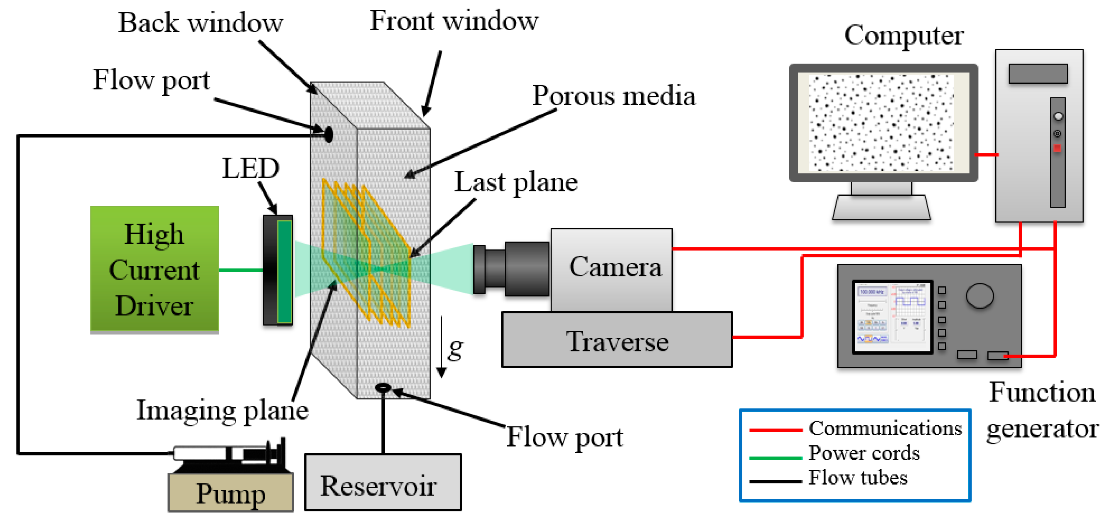
A schematic of the experimental setup used for shadowgraphy experiments is demonstrated in Figure 1. The liquid is pumped from the reservoir to the test flow cell using a syringe pump (‘11′ Plus, Harvard Apparatus Inc., Holliston, MA, USA), where the flow rate is set to 15 mL/h. The test flow cell has been fabricated using a commercial laser cutter (VersaLaser VLD Version 3.50; Universal Laser Systems, Scottsdale, AZ, USA). The flow cell is made up of Polymethyl methacrylate (PMMA) (Optix Acrylic; Plaskolit Inc., Columbus, OH, USA) and is confined with two side windows. The cell dimensions are 5.8 × 38.5 × 10 mm3 (d × h × w) at the porous media location. The flow cell is mounted vertically between a camera and a light source, and the flow is injected from one port on the cell and exits from the other flow port.
2.2. Imaging System
A shadow illumination and imaging system was used in the experiments to measure the flow. As shown in Figure 1, the imaging system utilized consisted of an LED light source (BX0404, Advanced Illumination Inc., Rochester, NY, USA) and a CCD camera (CMOS SP-5000M–PMCL, JAI Inc., Copenhagen, Denmark) that is capable of capturing up to 137 frames per second, with a resolution of 2000 pixel × 1800 pixel. For the micro-scale velocity measurements, an infinity corrected microscopic lens (Olympus Plan N × 4/0.10) was attached to an infinity corrected microscope (InfiniTube FM-200, Infinity Photo-Optical Co., Centennial, CO, USA). The optical lens assembly was calibrated and provided a field of view of 2.37 mm × 2.13 mm and a depth of field of ~0.08 mm. For the macro PIV measurements, a macro lens (Tamron SP 90 mm, f/2.8) was used which created a field of view equal to 8.6 mm × 10 mm. The images were processed using the commercial software DaVis 8.4.0 (LaVision GmbH, Göttingen, Germany). A function generator (AFG3021B, Tektronix Inc., Beaverton, OR, USA) was used to synchronize the camera and control image acquisition rate.
The experiments were performed in two stages. At the macro scale, the velocity was only measured in 2D to understand the overall pattern of the flow inside the flow test cell filled with porous media and to evaluate the appropriateness of the RIM technique for a large field of view measurement. It was also performed to evaluate the presence of the 3D motion of the fluid within the pore. Therefore, in macro-scale measurement, the medium was set to be in the field of view included both the flow port (where the extreme events were observed) and a point far from where the extreme events were observed in the test cell. For this set of imaging, the camera was focused at the mid-plane of the test flow cell with nearly the same distance from the front and back windows shown in Figure 1.
For 3D micro-scale velocity measurement, images were captured at different depths within a small volume in the flow cell consisting of a few glass beads and by moving the camera with respect to the flow cell and hence changing the focal plane location. This is shown schematically in Figure 1 as different imaging planes inside the porous media and in Figure 2 for images captured in the experiments. A fine pitch micrometer adjuster (148-801ST; Thorlabs, Newton, NJ, USA) with a translation rate of 6 μm/step was used to move the camera to the imaging locations. Data sets of 500 sequential images were collected at a frequency of 25 Hz at each depth, with an exposure time of 150 µs. Therefore, each plane resulted in 500 frames consisting of images of particles traced inside the porous media. Figure 2 shows the imaging approach in 3D flow measurement in more detail. A set of six planes, (a) to (f), is shown in Figure 2 with a typical image out of 500 at each plane. The out-of-plane coordinate ( axis) is originated at the front window and it is positive toward the back window. The positions of the planes shown in Figure 2 are listed in Table 1.
2.3. Porous Media
The porous medium in the current research is made of transparent spherical borosilicate glass spheres (Sigma-Aldrich, Z273619, St. Louis, MO, USA) to allow refractive index matching. Borosilicate glass beads have been reported [33] to have a constant and homogeneous index of refraction. The beads have an average size of 1 mm in diameter and the reported index of refraction of 1.470 to 1.473 at sodium D line [34,35]. The porosity of the medium was measured using the volume of the fluid and the cell volume to be 0.48. Prior to the experiments, the glass beads were washed using hydrochloric acid (HCl), rinsed with distilled water and dried at room temperature with natural convection. This was to remove the potential contamination from the surfaces of the beads, which might affect the flow and tracing particle behavior and imaging process. The beads showed no tendency to attract the tracing particles and did not absorb the test liquid or dissolve in it. The glass spheres are added to the flow cell to form a randomly packed porous media.
2.4. Refractive Index Matching Procedure
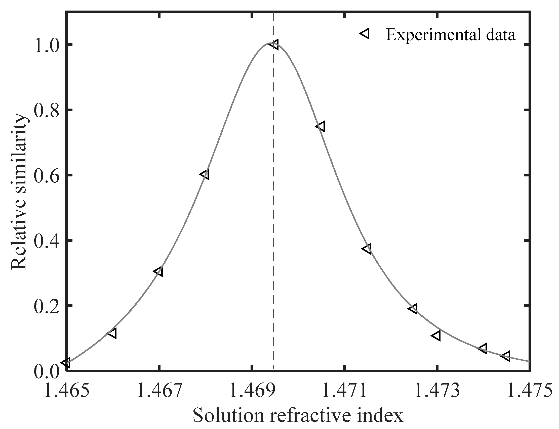
The reported refractive index for the beads covers a relatively large range. However, for flow measurement purposes, the refractive index should be less than 0.002 [18]. Therefore, to match the refractive index of the porous media and the liquid, the beads refractive index should be known. This sometimes becomes challenging due to the discrepancy between the reported and actual refractive index of manufactured materials of the individual beads, which is due to the changes to the refractive index during manufacturing procedures. Since there is no equipment for direct measurement of the refractive index of spherical particles, a new imaging approach was developed in this research. This was based on shadow imaging and comparing the image captured from the porous media soaked in a liquid with a reference image captured having no beads and only the liquid in the test cell. This shadow imaging technique was undertaken for a range of liquid refractive indices and a set of images was captured. Ideally, when the refractive index is matched, the beads become invisible and the shadow image is exactly similar to the reference image. However, there is some discrepancy between the shadow and reference images in practice. Therefore, the similarity of the images to the reference image should be evaluated. Details about calculation of image similarity techniques can be found in [36]. From the image set, the image that has the maximum similarity to the reference image is the one that is captured at matching refractive index. Hence, the associated liquid index of refraction is considered as the porous media refractive index. In the RIM procedure, a KSCN (Potassium thiocyanate)–water solution was used as it covers a range of refractive indices from 1.33 to 1.49 at different salt concentrations [33].
Figure 3 shows the relative similarity (to the maximum similarity) of 11 images (experimental data points) for the liquid refractive indices vary from 1.465 to 1.475. The image similarities have been normalized using the maximum similarity among the data set and represented by relative similarity in the figure. In Figure 3, the maximum relative similarity is observed at the refractive index of 1.4695, as shown with a dashed line. Therefore, velocimetry experiments are undertaken using a liquid that has the same refractive index as glass beads and satisfies the other flow requirements for the flow measurements such as liquid viscosity and density.
2.5. Test Liquid and Seeding Particles
Knowing the refractive index of the porous medium, experiments were performed using Canola oil. The refractive index of canola oil was measured in the lab and it had a similar refractive index as that of the glass beads in the porous media (1.4700). The specifications of the oil are listed in Table 2. The incompressible oil was seeded with 8 µm glass sphere tracer particles for the velocimetry purpose. The concentration of the seeding particle was set considering the requirements for flow measurement in porous media [37]. To achieve uniform distribution of the seeding particles in the oil and to avoid particle agglomeration, the mixture was stirred using a magnetic stirrer for at least 5 min.
2.6. Image Processing Method
The image processing method is slightly different between micro- and macro-scale velocimetry. For macro-scale velocimetry, the images were assessed with by averaging the information of the background images to determine the effect of potential light reflection on the background noise. Particle intensity counts were higher than the averaged image intensity counts and, therefore, light reflection did not influence the velocimetry. Using commercial software (DaVis 8.4.0, LaVision GmbH, Göttingen, Germany), a “subtract sliding” minimum was applied to the inverted images to eliminate non-uniform light intensity. This applies a high-pass filter and allows particle signals with small intensity fluctuation to pass while removing the large intensity fluctuations. A certain value was subtracted from the intensity counts of the entire image to set the intensity counts of the fluid image to zero. It should be noted that a geometric mask was also implemented to mask the undesired regions from contributing to vector calculation.
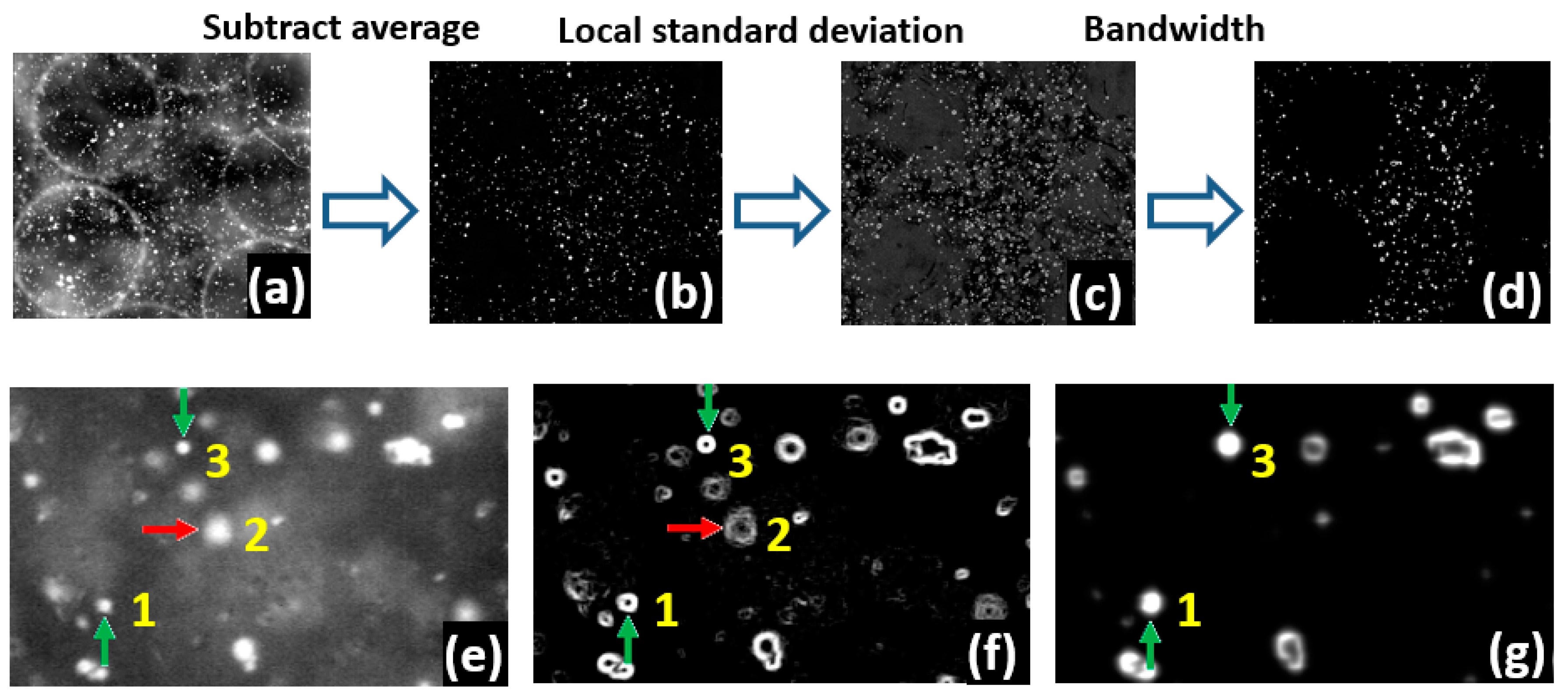
For images used at the micro scale to obtain subpore information, the unwanted out-of-focus particles needed to be eliminated from the images to attain more precise velocity vectors. The main steps undertaken in the image pre-processing are shown in Figure 4a–d and detailed by showing zoomed-in particles in Figure 4e–g. However, there are other minor steps, which are not discussed in these figures. For example, to remove the constant noise from the images, for each imaging plane, the minimum of 500 images is subtracted from all original images. The amplification of the intensities after subtracting a certain value from the intensity counts is another step that has been applied for noise removal, which has not been shown here.
A great portion of the out-of-focus particles can be removed by a thresholding filter as their intensities are lower than those of the in-focus particles. However, this does not always occur and sometimes the out-of-focus particles are included in the analysis after applying this filter [39] and will, on occasion, introduce errors in the velocity calculation. For instance, particles 1 and 3 in Figure 4e are in-focus particles while particle 2 is an out-of-focus particle. This is inferred from the fact that particle 2 moves more slowly than the in-focus particles that are located in the 2D image on both sides of it. Looking at the inverted image in Figure 4e, the maximum intensity of particle 1 which is an in-focus particle is 234 counts, while that of particle 2 which appears to be an out-of-focus particle is 254 counts. Thus, if a thresholding filter is used to remove the out-of-focus particles, regardless of the strength of the filter, particle 2 always remains longer than particle 1 in the processed image and results in producing erroneous velocity vectors (outliers).
As an alternative method to avoid this problem, the local standard deviation for each pixel was calculated by considering the 3-by-3 pixels in the neighbor around the corresponding pixel as shown in Figure 4f. This parameter is large for the pixels that have a remarkable contrast with their neighbors. As shown in Figure 4f, the more a particle is in focus, the brighter the circle surrounding the particle is. Therefore, while particles 1 and 3 are smaller than particle 2, they appear with higher intensities in Figure 4f. Despite adjusting the intensity of the in-focus particles, out-of-focus particles are in the image and further processing is required to make them invisible. This is performed by subtracting a certain value from the values of the local standard deviation to remove almost all the out-of-focus particles and identify the in-focus particles, which are shown in Figure 4g. While particle 1 and other in-focus particles are clearly visible in this figure, particle 2 has disappeared. It should be noted that in Figure 4g, the open circles were further filled by using a bandwidth filter to make them ready for performing a PTV algorithm. An animated example of particle tracking is shown in Figure S1 as supplementary material to this paper.
2.7. Velocimetry Procedure
For the macro-scale velocimetry, the velocity components and in the and directions were obtained using a standard particle image velocimetry (PIV) technique. The motion of the tracer particles within the sequence of the pre-processed images was calculated using a multi-pass sequential cross-correlation algorithm with decreasing window size (32 × 32 to 16 × 16 pixel2). First and second interrogating windows were used with three and one passes, respectively, and 75% window overlap in between sequential correlations. By applying the knowledge about the expected physics of the flow in the test geometry, such as smaller velocity vectors near the solid surfaces and larger velocity vectors in narrow paths, the results were evaluated. This is mainly to confirm that the velocimetry process has been properly applied and the results do not violate the physical laws.
After pre-processing the images for subpore velocimetry, a particle-tracking velocimetry (PTV) algorithm was applied. In this step, particles were detected based on a certain intensity threshold followed by the detection of the local maxima within a kernel of 17 × 17 pixel2. A band-passed filter was applied to the detected particles to accept only particles with a diameter within the range of 3 to 30 pixels. The location of each particle was determined with a Gaussian subpixel fit estimator [32] analyzed on a frame-by-frame basis to track individual colloidal particles. The data were filtered by limiting the magnitude of the displacement of particles to be smaller than 14 pixels in the horizontal direction () and 15 pixels in the vertical direction (). The maximum displacement gradient allowed in the vector field was set to 0.07 pixel/pixel, suggested as the maximum valid value [40]. Since the raw velocity data obtained from the PTV were sparse and randomly distributed across the image plane, the velocity in the empty pixels was estimated using a two-dimensional cubic interpolation algorithm (MATLAB R2017b, The MathWorks Inc., Natick, MA, USA).
Applying the planar PTV algorithm, the velocity vectors were calculated for each imaging plane. In this 3D velocimetry, the measurement was performed using the information obtained in the planar flow measurement and calculating the out-of-plane velocity components. This can be performed by reconstructing the volume using a 3D cross-correlation or through combining the planar velocimetry algorithm with the continuity equation [41]. The latter is used in this paper.
The out-of-plane position () of the measurement can be defined by the position of the focal plane and its resolution by the depth of focus. By illuminating the entire test cell and a using a stepwise approach to move a thin focal plane over the depth of the porous medium (as shown in Figure 1), 2D images of the tracer particle motion at several depths of the volume can be collected. The average out-of-plane component of the velocity () in each layer is then calculated from continuity of an incompressible liquid as:
where , and are known velocity components, and are the in-plane coordinates (obtained from 2D velocimetry), and is the out-of-plane coordinate. The above differential equation may be solved numerically, since the numerical values of and are known at discrete points in the volume.
By performing a planar PTV for each layer in the volume, the in-plane components of the velocity (,) and subsequently the velocity gradients, and are obtained. The variation of the third velocity component in the depth in each plane, , can be then calculated from Equation (1). Finally, the values of in each plane are determined from a linear extrapolation between the point with a known and the point of interest by assuming that the velocity components (including the out-of-plane component, ) at the solid are zero. Therefore,
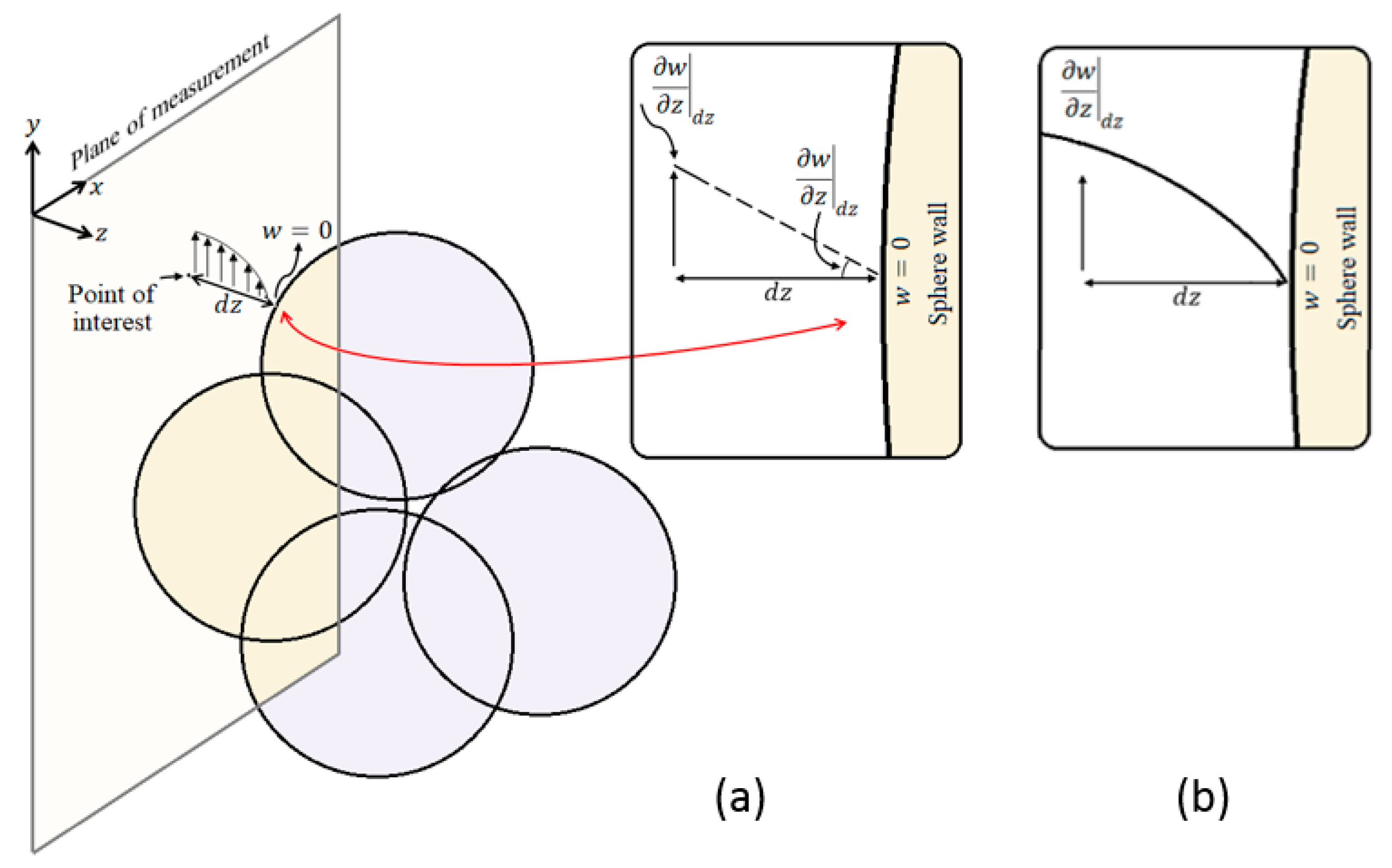
where is the distance between the point of interest and the solid wall. To calculate in each plane, the distance from the closest solid wall to the point on the plane was calculated. Further, the distance between the plane and the corresponding point located in the previous plane for which known was calculated. The value of is then calculated by considering the velocity of the closer point (either solid wall with = 0 or the point located at the previous plane with known ). Further details about the procedure can be found in [41]. Figure 5a shows how the continuity equation can be used to calculate from the in-plane components and .
It is important to highlight that the velocity field in this research was obtained using a first-order approximation for the out-of-focus component relation with respect to its gradient. This can be further improved by using higher-order polynomial approximations to calculate the out-of-plane velocity as shown in Figure 5b. This, however, involves a series of equations, which in turn significantly increases the computational efforts to obtain the velocity component. The linear approach is only considered in this research.
Using this approach, at each imaging plane, the velocity component is obtained by averaging the information from 500 frames collected at that plane. This resulted in 497 vector fields (2D) in each -plane and therefore, by combing the images and the continuity equation, a dense vector field was obtained. For the image planes shown in Figure 2, this is shown visually in Figure 6, where a dense vector field has been generated for plane (c).
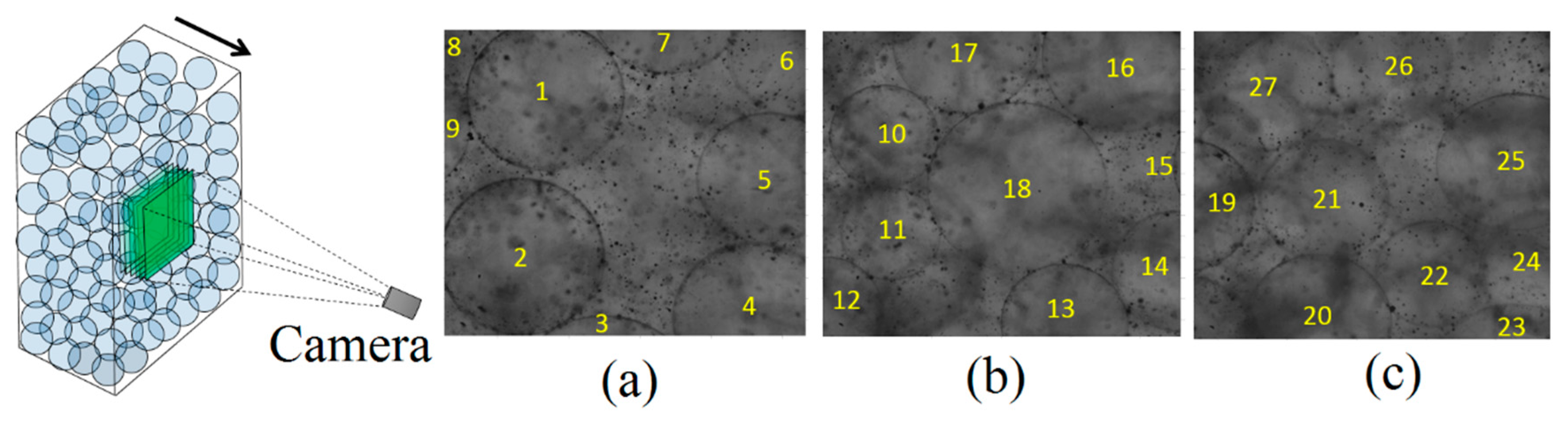
In order to calculate at each point in the space by using the velocity gradients obtained from Equation (1), the position of the closest solid wall to that point should be known. The location of the solid spheres in the space as well as their radii were obtained by slowly moving the flow cell in 6 µm intervals. The locations of the sphere centers with respect to the front window were approximated when the images of the spheres became sharp. For example, Figure 7a–c show the images captured at 3 different depths in the volume. Each individual sphere was labeled with a number and its central locations and radii were stored in a matrix. At each plane in the depth, the distance between the closest sphere surface as well as the distance to the front window was calculated. The minimum of these two values was considered as at that point to be used in Equation (2). In Figure 7, the sphere radii and locations were determined from the images in which they appeared sharp. In plane (a), spheres 1, 2, and 3 have a sharp edge. Therefore, their centers are assumed to be at plane (a). Similarly, plane (b) determines the positions of spheres 13 and 18, and plane (c) shows the positions of spheres 19, 20, and 25.
3. Results and Discussion
3.1. Macro-Scale 2D Velocimetry
Figure 8a shows an image of the flow cell when flow passes through it. The flow cell has a flow port which is 0.7 mm in width. The interface of the porous media and the fluid can be slightly detected for some particles despite the RIM of two phases. Such particles are seen as relatively dark in the image. Considering the bead surfaces have been decontaminated, this can be due to the non-uniformity in the refractive properties of the beads that make the refraction. To enhance the tracking procedure, the images are inverted and pre-processed as shown in Figure 8b. In the pre-processing, the stationary parts of the flow domain where the flow reaches the bead surfaces are calculated within images and the resulting image is subtracted from the raw images. As shown in Figure 8b, the white dots represent the tracer particles, which are moving in the flow field, and the black regions in the flow cell between the white dots are the stationary locations. The edge of the pores cannot be detected in this picture and only the path of the fluid motion can be seen. This process helps to achieve better detection of the tracer particles moving in the focal plane. The effect of the interface of the porous media on the velocity calculation can also be eliminated.
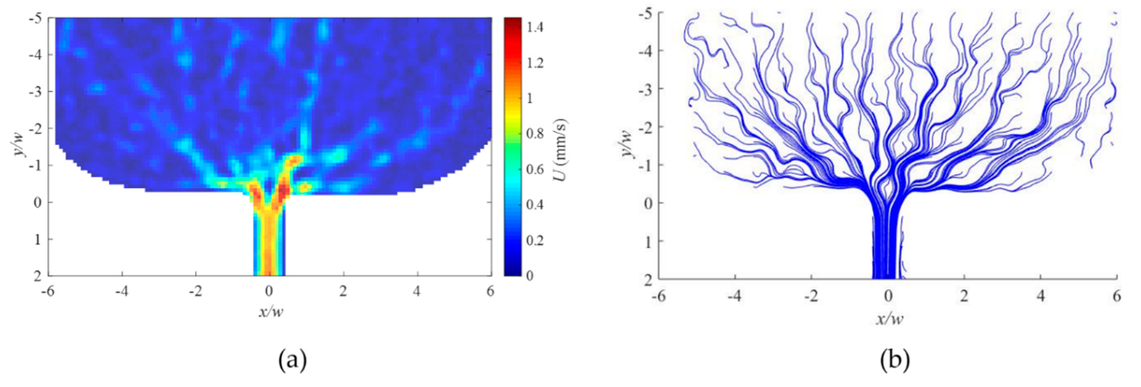
The velocity vector map obtained from 2D PIV for this case is shown in Figure 9a. The velocity vectors are normalized by the maximum velocity of the fluid in the field. Location is also normalized by the width of the flow port. The origin of the field is located at the bottom flow port on the centerline of the test cell. The velocity color map shows that the fluid has a higher velocity within the pore space between the pores. The zones with no motion, which represent the pores, can also be seen on this map. The bulk motion of the fluid accelerates as it moves closer to the flow port due to the decrease in the available cross-sectional area. It reaches its maximum velocity in the region before it enters the port. As shown in Figure 9a, there are regions with high velocity where they decelerate to zero velocity in the field. These regions represent out-of-plane motion of the fluid, which confirms the presence of 3D motion of the fluid within the pore.
The motion of the fluid within the pore can be further studied by the streamlines as shown in Figure 9b. It can be seen that particles within the pores move through different paths approaching the flow port. The streamlines are more dispersed in the upper region where the fluid moves with lower velocity. A smaller distance between the streamlines is observed in the locations representing higher velocity. Similarly, the regions with dense streamlines match the location with high velocity values represented in Figure 9a. However, the streamlines provide a clearer visualization of the flow pattern inside the medium and flow paths. The streamlines converge, as they are closer to the exit, resulting in the smallest distance between them, which indicates the highest velocity at this location.
For the values of density = 925 kg/m3, the maximum velocity measured in the volume ≈ 0.65 × m/s, maximum pore size = m, and viscosity = 0.043 Pa·s, the Reynolds number () calculated was found to be in the order of ≈ 0.01. Therefore, the viscous forces are dominant, and the flow may be categorized into a laminar flow. Further, it is assumed that the gravitational and the pressure forces do not change during the image recording (~20 s). Therefore, the flow could be considered a steady flow.
3.2. Micro-Scale 3D Velocimetry
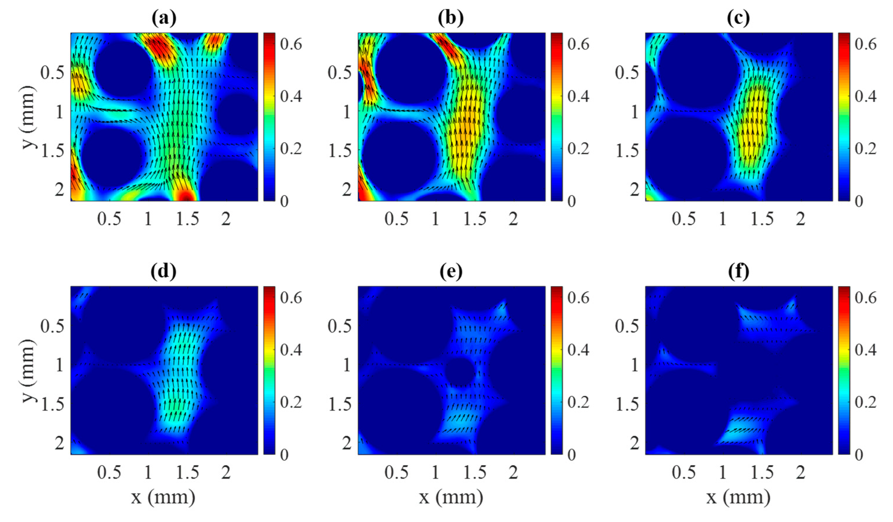
The in-plane velocity components obtained from the 2D PTV processing discussed earlier are shown in Figure 10. The different panels in Figure 10 show the velocity field at different depths of the porous medium, with panel (a) being the closest to the front window of the test cell.
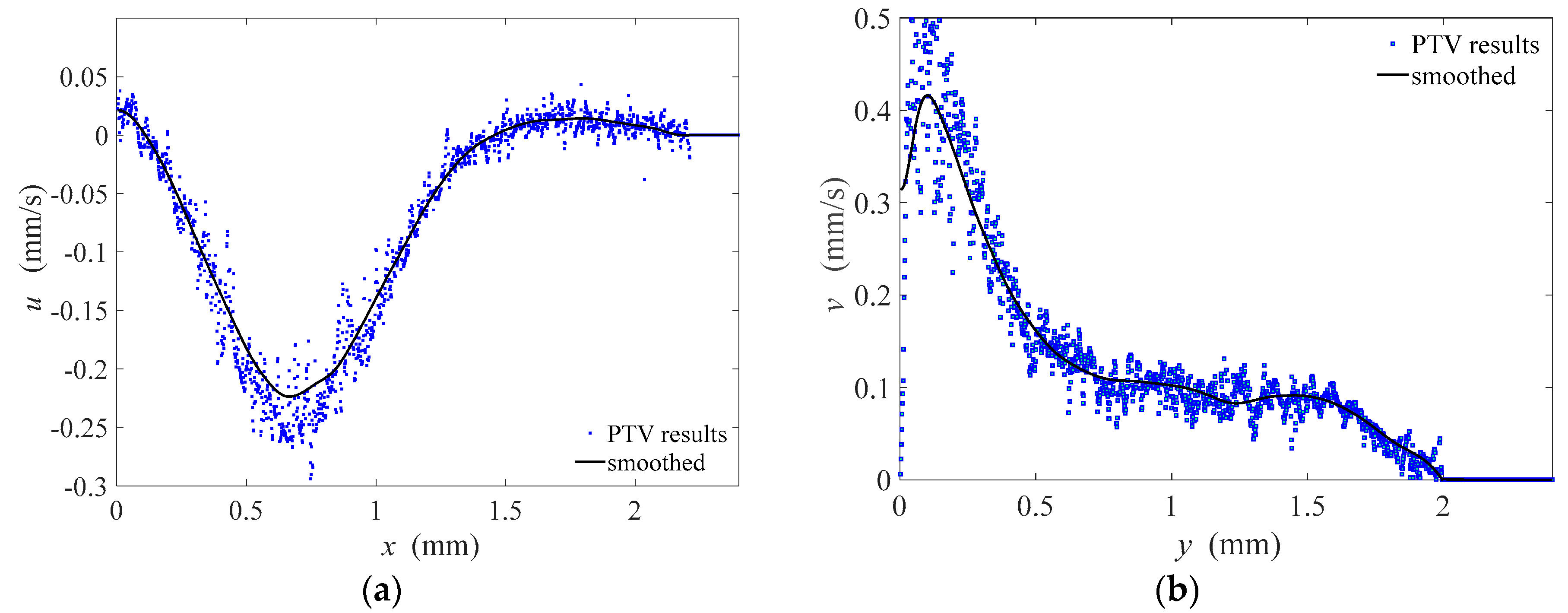
As shown in Figure 10, the fluid accelerates in the narrower regions, satisfying the continuity equation, Equation (1). By comparing Figure 10a–f, it appears that the magnitude of the in-plane velocity vectors () diminishes by increasing the distance from the front window that is located at = 0 (see Figure 2). This implies that the liquid flows faster near the window compared to the central region of the porous medium that can be due to the smaller resistance against the flow near the side windows. The out-of-plane component of velocity () at different planes was computed from the continuity equation, Equation (1). As calculated from this approach strongly depends on the gradients of the in-plane velocities ( and ) rather than the velocities (,) themselves (see Equation (1)), the in-plane velocities (,) need to be smoothed before being introduced into Equation (1) to get a coherent from the continuity equation. Figure 11a,b show a comparison between the smoothed velocity profiles and the non-smoothed ones obtained from PTV. Smoothing was performed using a 2D smoothing function [42]. As Figure 11a,b show, the smoothing algorithm captures a consistent pattern in the velocity data sets and eliminates the outliers that cause a sharp and noisy variation in the gradients of the velocity. By using the smoothed gradients and Equation (1), can be calculated. It is worth noting that the smoothing algorithm used here may not provide a reliable result at the boundaries (see y → 0 in Figure 11b for instance) and may not preserve the actual values of the velocity gradients in those regions. Therefore, the calculated and therefore w may not be reliable at the boundaries.
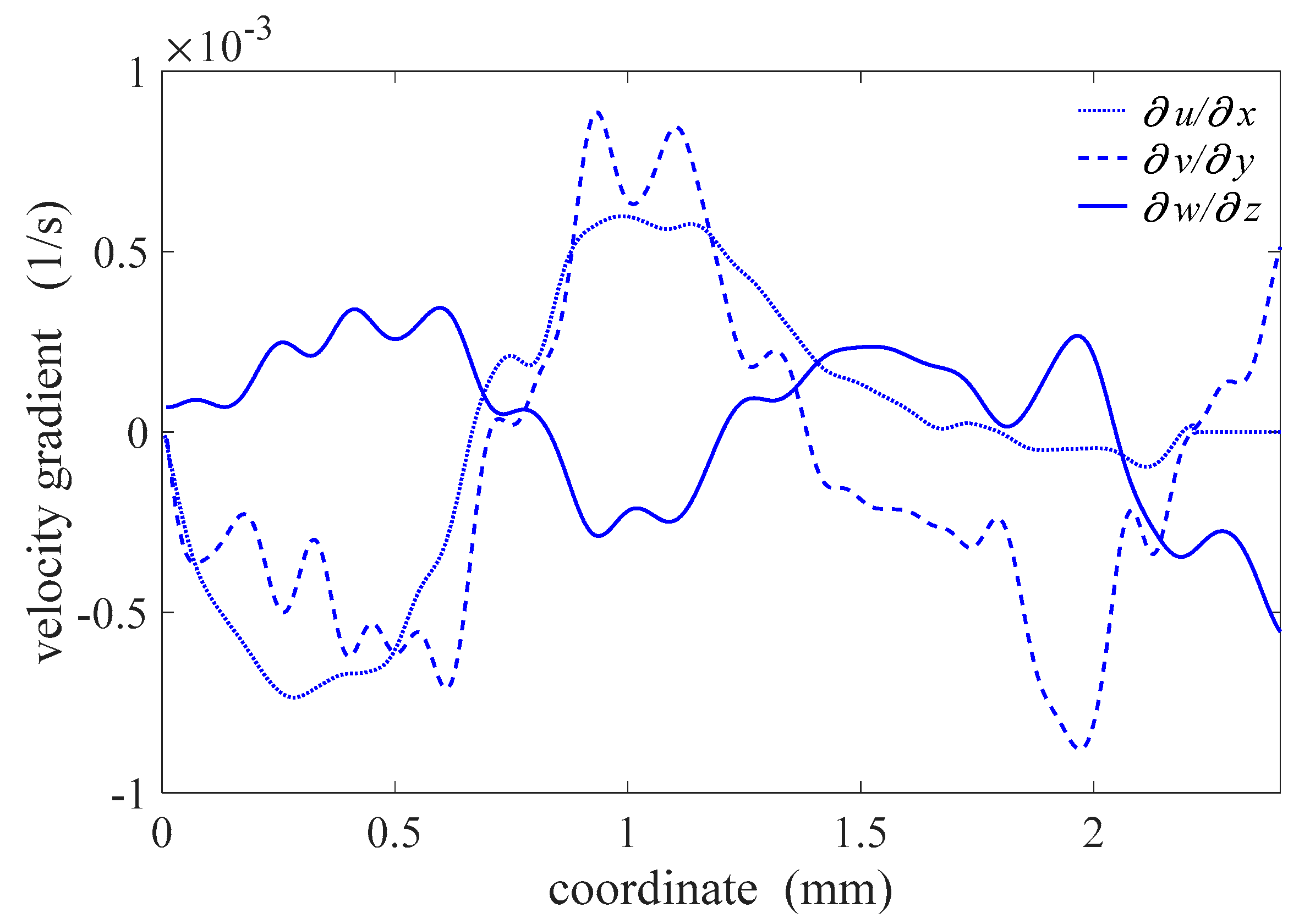
An example of the velocity gradients in different directions is shown in Figure 12 for one selected plane for each direction. As shown in the figure, the smoothed planar velocity gradients resulted in a velocity gradient for out-of-plane velocity component. Clearly, the velocity gradients in this figure are not associated with adjacent grids as they have been plotted against the relevant directions and hence one should not expect to use the and values in this figure to achieve the plotted values. The figure helps achieve an understanding of the magnitude of the velocity gradients for each component.
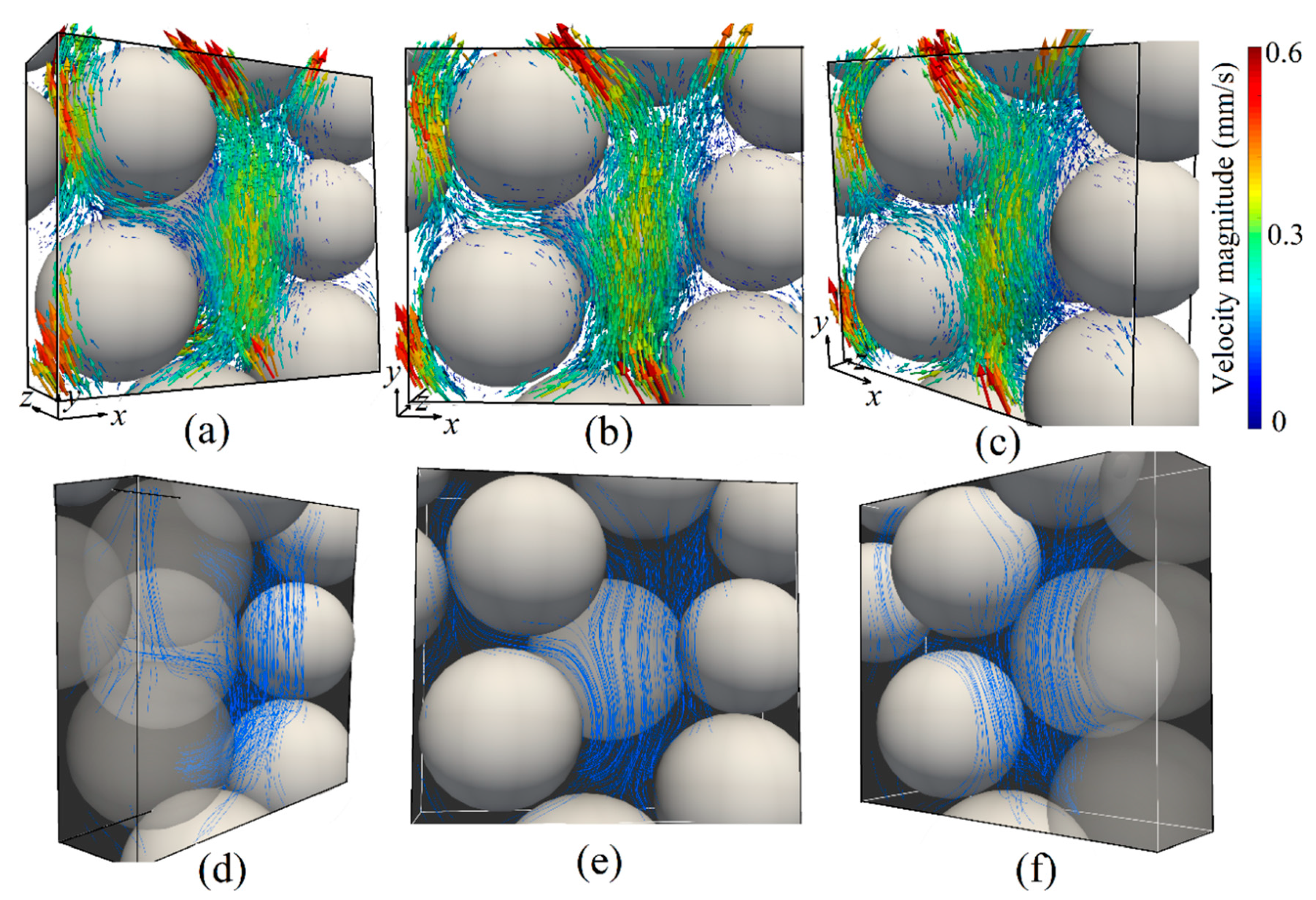
Plots in Figure 13a–c show the velocity vectors developed from the experimental measurement in the volume and the vectors for each velocity component. Here, the location of the spheres forming the porous media are identified from the image and velocity data and a virtual sphere is sized and positioned within the 3D velocity field. As expected, the velocity magnitude is higher in narrower pores between the beads. The maximum velocity observed in the experiments is 0.64 mm/s. The pore shown in the middle of the images (a–c) is relatively large compared to the other pores, which results in approximately 50% reduction in velocity magnitude comparing the maximum velocity in the porous media that is under investigation. Figure 13d–f represent some of the streamlines inside the porous media for three different perspectives reconstructed from the images and the velocity vectors obtained from the experiments. The streamlines are the lines that are tangential to the instantaneous velocity vectors. For the ideal tracer particles (massless particles), streamlines represent the paths of the tracer particles. The 3D animated velocity fields with the projection of the velocity vectors in all coordinates and positions and for each velocity component are provided as the supplementary material to the paper in Figures S2 and S5.
4. Conclusions
Using a new approach to obtain the refractive index matching of a porous medium, the 2D and 3D flow of oil is measured non-intrusively through the pores of randomly packed borosilicate spherical glass beads. Flow behavior in porous media is investigated at the macro scale and the 3D flow is confirmed. Using a shadow imaging approach, the refractive index of the medium is detected and matched with the test fluid. Both micro- and macro-scale velocity measurements are undertaken using the PIV technique for flow measurement at the macro scale. At the micro scale, the flow is measured in the subpore of the porous media using a planar PTV algorithm combined with the law of conservation of mass. Details about the particle detection and removing out-of-focus particles have been discussed. The in-plane velocity components at different depths of the porous medium are obtained by the time tracking of the individual particles in the flow. To obtain the out-of-plain component of the velocity, the continuity equation is employed. An improvement to the velocity calculation would be achieved if a thinner depth of focus is used. The use of the continuity equation combined with the result of 2D PTV shows promising results to determine the full velocity information in the volume using only a single camera. However, the smoothing algorithm applied to the in-plane velocities in this study did not provide a reliable result at the boundaries. As a result, further investigation is needed on how to treat the noisy velocities obtained from 2D PIV/PTV and therefore to improve the calculated out-of-plane velocity. A possible remedy may be fitting a polynomial to the 2D data instead of smoothing them. It is also important to mention that the application of the continuity equation relies on the presence of solid walls at which the velocities are known. If the volume of interest is far from a solid wall, this technique may need to be combined with other 3C3D techniques or, otherwise, it may not give a fair estimation of the out-of-plane velocity. Nevertheless, the application of the continuity equation has great potential to be employed in other applications where implementation of the 3D velocimetry measurements is difficult. However, this approach needs to be further explored and developed in the future by comparing it to the results from other existing approaches such as tomographic PIV and defocusing PTV. The high spatial and temporal resolution are of the advantages of the technique implemented in this research.
Supplementary Materials
The following are available online at https://0-www-mdpi-com.brum.beds.ac.uk/2673-3269/1/1/6/s1. Figure S1: Example of particle detection and tracking; Figure S2: 3D rotation of measurement volume including beads, subpores and velocity vectors; Figure S3: 3D velocity vectors with velocity projection in plane scanning along the direction; Figure S4: 3D velocity vectors with velocity projection in plane scanning along the direction; Figure S5: 3D velocity vectors with velocity projection in plane scanning along the direction (in pixel scale).
Author Contributions
Conceptualization, D.S.N.; methodology, R.S., M.A.K., H.S., and D.S.N.; software, R.S. and M.A.K.; validation, R.S., M.A.K., and D.S.N.; formal analysis, R.S. and M.A.K.; investigation, R.S., M.A.K., and H.S.; resources, D.S.N.; data curation, R.S. and M.A.K.; writing—original draft preparation, R.S. and M.A.K.; writing—review and editing, R.S., M.A.K., and D.S.N.; visualization, R.S. and M.A.K.; supervision, D.S.N.; project administration, D.S.N.; funding acquisition, D.S.N. All authors have read and agreed to the published version of the manuscript.
Funding
This research received no external funding.
Acknowledgments
Financial support from the Canada Foundation for Innovation (CFI), the Natural Sciences and Engineering Research Council of Canada (NSERC) is gratefully acknowledged.
Conflicts of Interest
The authors declare no conflict of interest. The funders had no role in the design of the study; in the collection, analyses, or interpretation of data; in the writing of the manuscript, or in the decision to publish the results.
References
- Wood, B.; Apte, S.; Liburdy, J.; Ziazi, R.; He, X.; Finn, J.; Patil, V. A comparison of measured and modeled velocity fields for a laminar flow in a porous medium. Adv. Water Resour. 2015, 85, 45–63. [Google Scholar] [CrossRef] [Green Version]
- Khaled, A.; Vafai, K. The role of porous media in modeling flow and heat transfer in biological tissues. Int. J. Heat Mass Transf. 2003, 46, 4989–5003. [Google Scholar] [CrossRef]
- Sahimi, M.; Imdakm, A.O. Hydrodynamics of particulate motion in porous media. Phys. Rev. Lett. 1991, 66, 1169–1172. [Google Scholar] [CrossRef] [PubMed]
- Fang, F.; Babadagli, T. 3-D visualization of diffusive and convective solvent transport processes in oil-saturated porous media using laser technology. J. Vis. 2016, 19, 615–629. [Google Scholar] [CrossRef]
- Roth, E.; Mont-Eton, M.E.; Lei, T.C.; Gilbert, B.; Mays, D. Measurement of colloidal phenomena during flow through refractive index matched porous media. Rev. Sci. Instrum. 2015, 86, 113103. [Google Scholar] [CrossRef] [Green Version]
- Vafayi, K. Porous Media: Applications in Biological Systems and Biotechnology; Taylor & Francis Group: Abingdon, UK, 2011. [Google Scholar]
- Ryan, J.N.; Elimelech, M. Colloid mobilization and transport in groundwater. Colloids Surf. A Physicochem. Eng. Asp. 1996, 107, 1–56. [Google Scholar] [CrossRef]
- Tilke, P.G.; Holmes, D.W.; Williams, J.R. Characterizing Flow in Oil Reservoir Rock Using Smooth Citation Accessed Characterizing Flow in Oil Reservoir Rock Using Smooth Particle Hydrodynamics. AIP Conf. Proc. 2010, 1254, 278–283. [Google Scholar]
- Reis, A.H.; Miguel, A.F. Transport and Deposition of Fine Mode Particles in Porous Filters. J. Porous Media 2006, 9, 731–744. [Google Scholar] [CrossRef]
- Huang, L.; Mikolajczyk, G.; Küstermann, E.; Wilhelm, M.; Odenbach, S.; Dreher, W. Adapted MR velocimetry of slow liquid flow in porous media. J. Magn. Reson. 2017, 276, 103–112. [Google Scholar] [CrossRef]
- Roth, E.; Gilbert, B.; Mays, D. Colloid Deposit Morphology and Clogging in Porous Media: Fundamental Insights Through Investigation of Deposit Fractal Dimension. Environ. Sci. Technol. 2015, 49, 12263–12270. [Google Scholar] [CrossRef] [Green Version]
- Vafai, K. Handbook of Porous Media, 2nd ed.; CRC Press: Boca Raton, FL, USA, 2005. [Google Scholar]
- Wiederseiner, S. Rheophysics of Concentrated Particle Suspensions in a Couette Cell using a Refractive Index Matching Technique; EPFL: Lausanne, Switzerland, 2010; p. 161. [Google Scholar]
- Khalili, A.; Basu, A.J.; Pietrzyk, U. Flow visualization in porous media via Positron Emission Tomography. Phys. Fluids 1998, 10, 1031–1033. [Google Scholar] [CrossRef]
- Werth, C.J.; Zhang, C.; Brusseau, M.L.; Oostrom, M.; Baumann, T. A review of non-invasive imaging methods and applications in contaminant hydrogeology research. J. Contam. Hydrol. 2010, 113, 1–24. [Google Scholar] [CrossRef] [PubMed] [Green Version]
- Harris, R.J.; Sederman, A.; Mantle, M.D.; Crawshaw, J.; Johns, M.L. A comparison of experimental and simulated propagators in porous media using confocal laser scanning microscopy, lattice Boltzmann hydrodynamic simulations and nuclear magnetic resonance. Magn. Reson. Imaging 2005, 23, 355–357. [Google Scholar] [CrossRef] [PubMed]
- Liyanage, R.; Cen, J.; Krevor, S.; Crawshaw, J.P.; Pini, R. Multidimensional Observations of Dissolution-Driven Convection in Simple Porous Media Using X-ray CT Scanning. Transp. Porous Media 2018, 126, 355–378. [Google Scholar] [CrossRef] [Green Version]
- Dijksman, J.A.; Rietz, F.; Lőrincz, K.A.; Van Hecke, M.; Losert, W. Invited Article: Refractive index matched scanning of dense granular materials. Rev. Sci. Instrum. 2012, 83, 11301. [Google Scholar] [CrossRef]
- Häfeli, R.; Altheimer, M.; Butscher, D.; Von Rohr, P.R. PIV study of flow through porous structure using refractive index matching. Exp. Fluids 2014, 55, 1717. [Google Scholar] [CrossRef]
- Frey, J.M.; Schmitz, P.; Dufrêche, J.; Pinheiro, I.G. Particle Deposition in Porous Media: Analysis of Hydrodynamic and Weak Inertial Effects. Transp. Porous Media 1999, 37, 25–54. [Google Scholar] [CrossRef]
- Harshani, H.M.D.; Torres, S.A.G.; Scheuermann, A.; Muhlhaus, H.B. Experimental study of porous media flow using hydro-gel beads and LED based PIV. Meas. Sci. Technol. 2016, 28, 15902. [Google Scholar] [CrossRef]
- Wiederseiner, S.; Andreini, N.; Epely-Chauvin, G.; AnceyiD, C. Refractive-index and density matching in concentrated particle suspensions: A review. Exp. Fluids 2010, 50, 1183–1206. [Google Scholar] [CrossRef]
- Wright, S.F.; Zadrazil, I.; Markides, C.N. A review of solid–fluid selection options for optical-based measurements in single-phase liquid, two-phase liquid–liquid and multiphase solid–liquid flows. Exp. Fluids 2017, 58, 108. [Google Scholar] [CrossRef]
- Beguin, R.; Philippe, P.; Faure, Y. Pore-Scale Flow Measurements at the Interface between a Sandy Layer and a Model Porous Medium: Application to Statistical Modeling of Contact Erosion. J. Hydraul. Eng. 2013, 139, 1–11. [Google Scholar] [CrossRef] [Green Version]
- Stöhr, M.; Roth, K.; Jähne, B. Measurement of 3D pore-scale flow in index-matched porous media. Exp. Fluids 2003, 35, 159–166. [Google Scholar] [CrossRef]
- Krummel, A.T.; Datta, S.; Münster, S.; Weitz, D.A. Visualizing multiphase flow and trapped fluid configurations in a model three-dimensional porous medium. AIChE J. 2013, 59, 1022–1029. [Google Scholar] [CrossRef]
- Holzner, M.; Morales, V.; Willmann, M.; Dentz, M. Intermittent Lagrangian velocities and accelerations in three-dimensional porous medium flow. Phys. Rev. E 2015, 92, 013015. [Google Scholar] [CrossRef] [PubMed] [Green Version]
- Moroni, M.; Cushman, J.H.; Cenedese, A. Application of Photogrammetric 3D-PTV Technique to Track Particles in Porous Media. Transp. Porous Media 2008, 79, 43–65. [Google Scholar]
- Guo, T.; Ardekani, A.M.; Vlachos, P.P. Microscale, scanning defocusing volumetric particle-tracking velocimetry. Exp. Fluids 2019, 60, 89. [Google Scholar] [CrossRef]
- Cierpka, C.; Kähler, C.J. Particle imaging techniques for volumetric three-component (3D3C) velocity measurements in microfluidics. J. Vis. 2011, 15, 1–31. [Google Scholar] [CrossRef] [Green Version]
- Fuchs, T.; Hain, R.; Kähler, C.J. In situcalibrated defocusing PTV for wall-bounded measurement volumes. Meas. Sci. Technol. 2016, 27, 084005. [Google Scholar] [CrossRef]
- Cavazzini, G. The Particle Image Velocimetry—Characteristics, Limits and Possible Applications; InTech: Rijeka, Croatia, 2012. [Google Scholar]
- Agrawal, Y.K.; Sabbagh, R.; Sanders, S.; Nobes, D. Measuring the Refractive Index, Density, Viscosity, pH, and Surface Tension of Potassium Thiocyanate (KSCN) Solutions for Refractive Index Matching in Flow Experiments. J. Chem. Eng. Data 2018, 63, 1275–1285. [Google Scholar] [CrossRef]
- University of Liverpool, Absolute Refractive Index; Materials Teaching Educational Resources. 2007. Available online: https://web.archive.org/web/20071012161040/http://matter.org.uk/schools/Content/Refraction/absolute.html (accessed on 25 February 2020).
- Parson, L.; (Chemglass Life Sciences LLC, Vineland, NJ, USA). Properties of Borosicate Glass Bead. Personal communication, 2014. [Google Scholar]
- Wang, Z.; Bovik, A. Modern Image Quality Assessment. Synth. Lect. Image Video Multimed. Process. 2006, 2, 1–156. [Google Scholar] [CrossRef]
- Patil, V.A.; Liburdy, J.A. Characterization of PIV Seed Particles for Flow in Porous Media. In Proceedings of the Processing and Engineering Applications of Novel Materials, Vancouver, BC, Canada, 12–18 November 2010; Volume 12, pp. 485–493. [Google Scholar]
- Ventura Foods. Ventura Foods Canola Oil Safety Data Sheet. 2015, pp. 1–7. Available online: https://www.venturafoods.com/wp-content/uploads/2019/03/VF-SDS-Canola-Oil.pdf (accessed on 25 February 2020).
- Benson, T.; French, J. InSiPID: A new low-cost instrument for in situ particle size measurements in estuarine and coastal waters. J. Sea Res. 2007, 58, 167–188. [Google Scholar] [CrossRef]
- Keane, R.D.; Adrian, R.J. Theory of cross-correlation analysis of PIV images. Flow Turbul. Combust. 1992, 49, 191–215. [Google Scholar] [CrossRef]
- Kazemi, M.A.; Elliott, J.A.W.; Nobes, D.S. Determination of the three components of velocity in an evaporating liquid from scanning PIV. In Proceedings of the 18th International Symposium on the Application of Laser and Imaging Techniques to Fluid Mechanics, Lisbon, Portugal, 4–7 July 2016. [Google Scholar]
- Reeves, G. Smooth2a Function v. 1.0 MATLAB File Exchange. Available online: https://www.mathworks.com/matlabcentral/fileexchange/23287-smooth2a (accessed on 13 March 2009).
Figure 1.
Schematic of the experimental setup. The camera-facing window is the front window and the LED-facing window is the back window. Examples of some imaging planes are shown.
Figure 1.
Schematic of the experimental setup. The camera-facing window is the front window and the LED-facing window is the back window. Examples of some imaging planes are shown.

Figure 2.
Schematic of the imaging planes and the porous media (left) and the sample images of each plane (right) where each image is a representative of 500 frames captured at its imaging plane. The axis is normal to the planes and positive toward the back window. The front window is assumed to be at = 0.

Figure 3.
Relative similarity of the images with the reference images captured at different KSCN solution refractive indices. Experimental data are shown along with the fitted curve. The maximum similarity is observed at the refractive index of 1.4695 shown with a dashed line.
Figure 3.
Relative similarity of the images with the reference images captured at different KSCN solution refractive indices. Experimental data are shown along with the fitted curve. The maximum similarity is observed at the refractive index of 1.4695 shown with a dashed line.

Figure 4.
The sequence of the main steps undertaken in the image pre-processing for removing the out-of-focus particles from the collected images and making them ready for performing particle-tracking velocimetry (PTV) algorithm. (a) Original inverted image, (b) image after subtracting the average, (c) applying local standard deviation, (d) final image after bandwidth filtering, (e) zoomed in inverted raw image with particles 1 and 3 in focus and particle 2 out of focus, (f) after applying the local standard deviation filter, particles 1 and 3 become brighter, and (g) after using a Bandwidth filter and removing particle 2. Some intermediate steps of image pre-processing such as subtracting the minimum of 500 images from all original images to filter out the constant noise or the amplification of the intensities after subtracting a certain value from the intensities to remove the noise are not shown here.

Figure 5.
Schematics showing how the continuity equation is applied to compute the out-of-plane velocity from its gradient using (a) a first-order approximation (b) a higher-order approximation could be used but it has not been employed in this study.
Figure 5.
Schematics showing how the continuity equation is applied to compute the out-of-plane velocity from its gradient using (a) a first-order approximation (b) a higher-order approximation could be used but it has not been employed in this study.

Figure 6.
Schematic of the steps performed in developing the dense vector field. Images from planar velocimetry in plane (c) resulted in 497 sparse vector fields that finally led to one dense vector filed at a certain position in the depth.
Figure 6.
Schematic of the steps performed in developing the dense vector field. Images from planar velocimetry in plane (c) resulted in 497 sparse vector fields that finally led to one dense vector filed at a certain position in the depth.

Figure 7.
The procedure to determine the location of spheres in the volume. The focal plane of the camera is slowly penetrated in the volume by displacing the porous medium toward the camera. In plane (a), spheres 1, 2, and 3 have a sharp edge. In plane (b) spheres 13 and 18, and in plane (c), the positions of spheres 19, 20, and 25 are obtained.

Figure 8.
(a) Raw image and (b) the pre-processed images of the 2D velocimetry in the flow test cell.
Figure 8.
(a) Raw image and (b) the pre-processed images of the 2D velocimetry in the flow test cell.

Figure 9.
(a) Velocity magnitude map from 2D velocimetry and (b) streamlines for the flow in porous media obtained after PIV processing.
Figure 9.
(a) Velocity magnitude map from 2D velocimetry and (b) streamlines for the flow in porous media obtained after PIV processing.

Figure 10.
Two-dimensional representation of the in-plane velocity components at different depths of the porous medium obtained from PTV. Panels (a)–(f) are shown in Figure 2 with the positions reported in Table 1. Color bars represent the planar velocity magnitude in mm/s.

Figure 11.
Examples of smoothing the in-plane velocity data obtained from PTV in order to calculate the out-of-plane component of velocity; (a) component and (b) component.
Figure 11.
Examples of smoothing the in-plane velocity data obtained from PTV in order to calculate the out-of-plane component of velocity; (a) component and (b) component.

Figure 12.
Example of velocity gradient plots obtained from the PTV results. Horizontal axis represents the corresponding direction for each velocity gradient that is or or .
Figure 12.
Example of velocity gradient plots obtained from the PTV results. Horizontal axis represents the corresponding direction for each velocity gradient that is or or .

Figure 13.
(a–c) The 3D vector field reconstructed from combining the 2D velocities obtained from PTV and out-of-plane velocities obtained from Equation (1). Different panels (a–c) show the same vector field from different perspectives. (d–f) A 3D representation of some selected streamlines within the volume from three different perspectives. The color bar represents the total velocity magnitude in mm/s.


Table 1.
Selected planes and their depths as shown in Figure 2.
Table 1.
Selected planes and their depths as shown in Figure 2.
| Plane | Depth (mm) |
|---|---|
| a | 0.24 |
| b | 0.34 |
| c | 0.44 |
| d | 0.54 |
| e | 0.64 |
| f | 0.74 |
Table 2.
Canola oil specifications [38].
Table 2.
Canola oil specifications [38].
| Parameter | Description |
|---|---|
| Physical state | Transparent liquid |
| Water solubility | Insoluble |
| Color | Light yellow |
| Flash point | >325 °C |
| Boiling point | No data available |
| Ignition point | >330 °C |
| Vapor pressure | <0.1 mmHg at 300 °C |
| Viscosity | 43 mPa·s at 35 °C |
| Specific gravity | 0.920–0.925 |
© 2020 by the authors. Licensee MDPI, Basel, Switzerland. This article is an open access article distributed under the terms and conditions of the Creative Commons Attribution (CC BY) license (http://creativecommons.org/licenses/by/4.0/).
Share and Cite
MDPI and ACS Style
Sabbagh, R.; Kazemi, M.A.; Soltani, H.; Nobes, D.S. Micro- and Macro-Scale Measurement of Flow Velocity in Porous Media: A Shadow Imaging Approach for 2D and 3D. Optics 2020, 1, 71-87. https://0-doi-org.brum.beds.ac.uk/10.3390/opt1010006
AMA Style
Sabbagh R, Kazemi MA, Soltani H, Nobes DS. Micro- and Macro-Scale Measurement of Flow Velocity in Porous Media: A Shadow Imaging Approach for 2D and 3D. Optics. 2020; 1(1):71-87. https://0-doi-org.brum.beds.ac.uk/10.3390/opt1010006
Chicago/Turabian StyleSabbagh, Reza, Mohammad Amin Kazemi, Hirad Soltani, and David S. Nobes. 2020. "Micro- and Macro-Scale Measurement of Flow Velocity in Porous Media: A Shadow Imaging Approach for 2D and 3D" Optics 1, no. 1: 71-87. https://0-doi-org.brum.beds.ac.uk/10.3390/opt1010006