
Resolution Limit of Correlation Plenoptic Imaging between Arbitrary Planes


1
Dipartimento Interateneo di Fisica, Università Degli Studi di Bari, I-70126 Bari, Italy
2
INFN, Sezione di Bari, I-70125 Bari, Italy
*
Author to whom correspondence should be addressed.
Optics 2022, 3(2), 138-149; https://0-doi-org.brum.beds.ac.uk/10.3390/opt3020015
Submission received: 7 March 2022
/
Revised: 1 April 2022
/
Accepted: 8 April 2022
/
Published: 12 April 2022
Abstract
:Correlation plenoptic imaging (CPI) is an optical imaging technique based on intensity correlation measurement, which enables detecting, within fundamental physical limits, both the spatial distribution and the direction of light in a scene. This provides the possibility to perform tasks such as three-dimensional reconstruction and refocusing of different planes. Compared with standard plenoptic imaging devices, based on direct intensity measurement, CPI overcomes the problem of the strong trade-off between spatial and directional resolution. Here, we study the resolution limit in a recent development of the technique, called correlation plenoptic imaging between arbitrary planes (CPI-AP). The analysis, based on Gaussian test objects, highlights the main properties of the technique, as compared with standard imaging, and provides an analytical guideline to identify the limits at which an object can be considered resolved.
1. Introduction
Plenoptic imaging (PI) identifies a category of devices and techniques characterized by the possibility of detecting the light field, namely the combined information on the spatial distribution and propagation direction of light, in a single exposure of the scene of interest [1]. The range of applications of PI is currently expanding, including, among others, microscopy [2,3,4,5], stereoscopy [1,6,7], wavefront sensing [8,9,10,11], particle image velocimetry [12], particle tracking and sizing [13], and photography, where it is employed to add refocusing capabilities to digital cameras [14]. Cutting edge applications include 3D neuronal activity functional imaging [5], surgery [15], endoscopy [16], and flow visualization [17]. In the state of the art, PI represents an extremely promising method to perform 3D imaging [18], because it gives the possibility of the parallel acquisition of 2D images from different perspectives, with only one sensor. State-of-the-art plenoptic devices are characterized by the presence of a microlens array in the image plane of the main lens. This additional component focuses on the sensor repeated images (one for each microlens) of the main lens [1,14]. These repeated images represent different perspectives of the illuminated object, which can be used to reconstruct light paths from the lens to the sensor, providing the possibility to refocus different planes in post-processing, change the viewpoint, and reconstruct images with a larger depth of field. However, the architecture of traditional plenoptic systems entails a trade-off between spatial and directional, the origin of which lies in the fundamental trade-off between the resolution and depth of field. Given a sensor with pixels per line and an array of microlenses per line, each corresponding to pixels per line behind, then . This imposes an increase by a factor in the linear size of the spatial resolution cell, which makes the diffraction limit, depending on the numerical aperture of the main lens, unreachable. Essentially, the resolution and depth of field that can be obtained by a standard plenoptic device are the same as one would obtain with an -times smaller numerical aperture of the main lens, entailing the practical (but not fundamental) advantage of a greater luminosity and signal-to-noise ratio of the final image, as well as the possibility of the parallel acquisition of multiperspective images.
In order to overcome this practical limitation, we recently developed and experimentally demonstrated a new technique, named correlation plenoptic imaging (CPI), capable of performing plenoptic imaging without losing spatial resolution [19,20]. In particular, the resolution of focused images can reach the physical (diffraction) limit. The system is based on encoding spatial and directional measurement on two separate sensors, by measuring second-order spatio-temporal correlations of light: the spatial information on a given plane in the scene is retrieved on one sensor [21,22,23,24,25], and the angular information is simultaneously obtained on the second sensor [26] thanks to the correlated nature of light beams [19,27,28]. As a result of such separation, the spatial vs. directional resolution trade-off is significantly mitigated. This technique paves the way toward the development of novel quantum plenoptic cameras, which will enable one to perform the same tasks of standard plenoptic systems, such as refocusing and scanning-free 3D imaging, along with a relevant performance increase in terms of resolution (which can be diffraction limited), depth of field, and noise [29]. In the first realizations of CPI, two particular reference planes, one inside the scene of interest, one practically coinciding with the focusing element, were imaged in order to reconstruct directional information. Such a task becomes non-trivial in the case of composite lenses, as those that one can find in a commercial camera or in a microscope, requiring the introduction of correction factors in the refocusing algorithms. We thus developed an alternative protocol, called correlation plenoptic imaging between arbitrary planes (CPI-AP), in which this difficulty is overcome by retrieving the images of two generic planes, typically placed inside the three-dimensional scene [30]. The proposed protocol highly simplifies the experimental implementation and improves refocusing precision; furthermore, it relieves the compromise between the resolution and depth of field, providing an unprecedented combination of them.
As in all CPI protocols, for technical and physical reasons that will be explained throughout this work, even in CPI-AP, it is not trivial to define resolution limits. Actually, the usual definition, based on a point-spread function, becomes immaterial in correlation plenoptic imaging. In this paper, we consider the paradigmatic case of objects characterized by a Gaussian profile, to identify reasonable definitions of a resolution limit. The analyticity of the results will provide a direct comparison, both qualitative and quantitative, with the case of standard imaging, based on direct intensity measurement.
2. Methods
In a second-order imaging protocol, light from a source is split (e.g., by a beam splitter) into two optical paths a and b, characterized by their optical propagators, that transfer the field from a point on the source, identified by the coordinates , to points of coordinates and on the detector planes. The correlation between fluctuations of the intensities and measured at the end of the corresponding paths generally encodes more information than the average intensities. The imaging properties of the correlation imaging device can be retrieved by the correlation function:
Intensity fluctuation correlations contain relevant information for imaging if light is chaotic or if the two beams are composed of entangled photons, produced, e.g., by spontaneous parametric down-conversion [21,28].
Let us now consider a typical setup of CPI-AP [30], shown in Figure 1. Light comes from an object, which emits chaotic light, propagates toward the lens , characterized by the focal length f, and then, encounters a beam splitter (BS). The latter generates two copies of the input beam, which are eventually detected by one of the two sensors and , both spatially resolving. The detectors are placed in such a way that they collect the focused images of two planes in proximity of the object, called and , respectively. As demonstrated in [30], plenoptic information can be retrieved by analysing the spatio-temporal correlations between the fluctuations in the intensity acquired by the two sensors. For evaluating in the discussed CPI-AP setup, we shall assume that the object is positioned at a distance z from the lens . Light emitted by this object is characterized by the intensity profile . We further assumed that transverse coherence can be safely neglected and that emission is quasi-monochromatic around the central wavelength (corresponding to the wavenumber ). In these conditions, propagation from an arbitrary point on the object plane to a point () on the detector () occurs through the proper paraxial optical transfer functions [31]. Neglecting irrelevant factors (independent of and , the resulting correlation function reads
where
with being the two propagators, the pupil function of the lens , and the magnifications of the object planes on detectors .
The plenoptic properties of from Equation (3) can be fully understood by considering the dominant contribution to the integrals in the limit of geometrical optics, which gives:
In this result, we observe that encodes at the same time images of the (squared) object intensity profile and of the lens pupil function P. While the latter is independent of the distance z between the lens and the object plane, the image of the object depends on the linear combination of the coordinates of the two detectors; if the object is placed in either of the planes or , will depend on the coordinates of only one detector, either or , respectively. This means that for (), does not depend any longer on (), and thus, integrating on () would provide a focused image of the object. As described in [30], when the object lies outside the depth of field around one of the two conjugate planes, integrating the correlation function on any detector plane coordinate would provide a blurred image. A “refocusing” algorithm, able to decouple the image of the lens from the image of the object, is therefore necessary; this is achieved by defining a proper linear combination of the detector coordinates and , such as the one given by the two variables:
The transformation in Equation (5) can be inverted and plugged into Equation (4), yielding the refocused correlation function:
with and satisfying the system of Equations (5). The effect of applying the transformation of Equation (5) to the argument of is thus to realign all the displaced images in order to reconstruct the focused image. We can now integrate the function over the variable, which gives:
In the limit , the above approximation tends to become exact, and the refocused image coincides with the squared object intensity profile. The refocusing procedure is robust against transverse alignment shifts:
of the two sensors with respect to the optical axes, since the effect on the refocused image (7) is a mere translation:
which does not affect the relative transverse distance between details nor the image resolution.
A natural benchmark for the refocused image of Equation (6) is represented by the images captured by the two detectors (with ) through direct intensity, namely:
In the limit, these quantities provide faithful images of the object profile:
only in the case . For different object positions, a geometrical spread of the image occurs, as we show in more detail in our case study.
3. Results
Due to the structure of the correlation function of Equation (2), the refocused image of Equation (7) takes the form
namely, it is a double integral on the object coordinates, with a proper function involving the optical propagators. Such a feature prevents us from defining a proper point-spread function, as one naturally does in the case of the direct intensity image. The resolution limits of CPI require a careful evaluation, and even ad hoc definitions. In fact, the plenoptic reconstruction of the direction of light in CPI-AP is based on imaging the two arbitrary planes focused by the lens on the detectors and ; a transmissive object acts as a diffractive aperture for such an image; hence, a point object would hinder the one-to-one correspondence between points of the plane and points of . To address this issue, we must test the behaviour of the refocused images of objects of a finite size. As a testbed, we consider a class of objects whose intensity profile is characterized by the Gaussian shape
of standard deviation a. This, also, allows performing an analytical determination of the refocusing function and a direct comparison of the results obtained in different cases. The lens aperture is modelled by the Gaussian pupil function:
which is often a good approximation for the pupil, especially for composite lenses. In this hypothesis, we first compute the correlation function Equation (2), which reads
with
where we used the shorthand notation
Then, following the refocusing procedure defined by Equations (5)–(7), we obtain the Gaussian refocused image
where coincides with the peak value. On the one hand, the width of this image can be expressed through the decomposition
where is the value obtained in the limit , providing a perfectly resolved image, as expected from Equation (7). On the other hand, the quantity
defines the spread due to the finite image resolution and is determined by factors such as the wavelength, the lens size , the distances of the two reference planes from the lens, and the object axial position z. It is worth noticing that the finite-resolution contribution depends also on the object width a, a feature not present in standard imaging, but already observed in other CPI cases, which we shall return to later. Based on Equation (11), the standard images of the object retrieved by each detector separately (see Equation (13)) reads
where
represents the effective magnification for an object at a distance z, rescaled by a geometrical projection factor , and
By inspection of the results of Equations (21), (22), and (25), we can outline the main differences between the two cases:
- While the spread of the direct intensity image is independent of a, the spread of the refocused CPI-AP image is monotonically decreasing with the object width. The dependence of the correlation image on the object is related to the role of as an “effective aperture” in correlation imaging;
- Consistent with the previous point, in Equation (22) is monotonically decreasing with the object size a. This entails that the total image width can have a counterintuitive non-monotonous behaviour with a, with a minimum for , unless the object is very close to one of the reference planes, namelyNoticeably, the value is always finite, unlike in previously analysed cases [20];
- As expected, in the out-of-focus case, the direct intensity image cannot provide a faithful representation of the object, even for ,since a residual purely geometrical spread, proportional to the lens aperture, is still present. Moreover, as the distance from the focused plane increases, the dependence of on a becomes progressively weaker, making objects of different widths indistinguishable. This is not the case for CPI-AP, since:refocusing provides a perfectly resolved image of , independent of the distance from the focused planes;
- The resolution and depth-of-field limits of traditional plenoptic imaging devices [14] are determined by the properties of the collected sub-images, obtained by reducing the main lens numerical aperture of a factor , with the number of directional resolution cells per line. Therefore, the image width is obtained by the replacementin Equation (25). Besides negatively affecting the resolution of the focused image, such a change entails a limitation to the image width at , which is qualitatively similar to the case reported in Equation (27) for standard imaging, although quantitatively attenuated.
The above considerations highlight both the enormous potential of the refocusing capability of CPI-AP and the difficulty of defining a resolution limit. In particular, the peculiar non-monotonic behaviour of the image size , which decreases with the object size when a comes close to zero, makes the definition of a point-spread function non-informative of the imaging capabilities of the system. To define a resolution limit, we followed the general idea that an object is resolved when the width of its image is at least approximately proportional to its own width.
Let us start from the case of a focused object, in which the image width takes the much simpler form
with the spread determined only by diffraction at the lens. For small a, the image width is dominated by the constant spread, and the size of the object can hardly be inferred from it. Instead, for large a, is essentially proportional to a, up to a small correction. A conventional transition point between the two regimes can be identified as the value of the object width, such that
namely, the value at which the width of the perfectly resolved image becomes equal to the spread. Incidentally, this value coincides with the minimum image width:
Motivated by these observations, we formulated two definitions to identify a lower limit to the object width that can be resolved, in the sense that it is proportional to the corresponding image width. The two definitions coincide in the focused cases .
First, by generalizing Equation (31), we define for an arbitrary object position z as the width value such that the perfectly resolved contribution to the image width becomes equal to the spread contribution:
By solving the above equation, we obtain
In Figure 2, we represent a graphical identification of , both in the case of (specifically, ), in which the spread is constant, and in the case (specifically, ), in which decreases with a, thus providing an even more reliable proportionality between image and object widths. In all plots, the parameters are fixed to , , , and .
The second definition of a lower limit for a resolvable object width a generalizes the quantity introduced in Equation (32), namely,
which coincides with in the special cases . This limit conventionally represents the value below which object widths are practically indistinguishable from each other. Its expression depends on the axial position z. Starting from the expression of the image width given in Equation (21), we find that in the limit , the quantity
corresponds to if the monotonicity condition in Equation (26) is satisfied; otherwise, the minimum occurs for
and
In Figure 3, we report a graphical identification of , both in the case (specifically, ), in which is monotonic with respect to a, and in the case (specifically, ), in which the minimum occurs for a finite value , and the image width increases with decreasing object width for .
A comparison between the two definitions of resolution limits for an object with a Gaussian intensity profile is reported in Figure 4, showing in the same plot the behaviour of and with varying z. The two quantities have consistent behaviours, with minima close to the two reference planes and a local maximum close to . While, as discussed before, the two limits coincide close to the focused planes, the limit tends to be more restrictive by a factor in the out-of-focus cases.
4. Discussion
We defined and discussed different characterizations of the resolution limits in CPI-AP for objects with a Gaussian profile. The difficulty in defining resolution limits in an unambiguous way has clearly emerged, since the two limit quantities that we considered, though coinciding in the focused case, deviate from each other as the object is placed away from the two reference planes. Specifically, the limit , which is obtained by imposing that the image width at perfect resolution is larger than the minimum image width, turns out to be generally more restrictive than the limit , which is obtained by requiring that the image width at a perfect resolution is larger than the spread due to the finite resolution.
The definition of resolution limits in the present work is conceptually different with respect to the one considered in the previous literature on the topic, which was based on the ability to discriminate a double slit with very specific features, namely a centre-to-centre distance equal to twice the slit width (see, e.g., [30] for the CPI-AP setup and [20] for a different CPI system). Despite this difference, the results obtained in our work are fully consistent with the previous ones in terms of the variation of the resolution with a varying object axial position. We remark that, though the present analysis highlights a better performance of CPI-AP in terms of resolution, a full evaluation of the advantages with respect to standard techniques must also take into account the problem of noise, which affects correlation imaging in a specific way (see, e.g., [32]). A thorough discussion of this issue will be a matter for future research.
An alternative approach to the investigation of further conventional resolution limits is to employ the modulation transfer function (MTF) criterion [33], in which the visibility of the image of a periodic intensity profile is analysed. This is outside the scope of the present paper, but we plan to investigate it in future research. In fact, we expect that the analytical results obtained with a sinusoidal profile can be exploited to provide a full control of the system performance.
Let us finally remark that the starting point of our analysis, namely the form of the correlation function given by Equation (2), relies on the physical assumption that the transverse coherence length on the source is much smaller than both the intensity profile extension and the linear size of the resolution cell defined by the lens. However, especially in a microscopy context, transverse coherence is not necessarily negligible and may affect the imaging properties of the device. Further research will be devoted to investigating how residual transverse coherence affects the resolution and depth of field of the CPI-AP system.
Author Contributions
Conceptualization, F.V.P. and M.D.; methodology, F.S. and F.V.P.; software, F.S.; validation, all authors; formal analysis, F.S.; investigation, F.S.; writing—original draft preparation, F.S.; writing—review and editing, all authors; visualization, F.S.; supervision, F.V.P. and M.D.; project administration, M.D.; funding acquisition, M.D. and F.S. All authors have read and agreed to the published version of the manuscript.
Funding
This research was funded by Research for Innovation REFIN—Regione Puglia POR PUGLIA FESR-FSE 2014/2020, INFN project PICS4ME, and MISE-UIBM project INTEFF-TOPMICRO.
Institutional Review Board Statement
Not applicable.
Informed Consent Statement
Not applicable.
Data Availability Statement
No new data were created or analyzed in this study. Data sharing is not applicable to this article.
Acknowledgments
The authors thank Francesco Di Lena for useful discussions.
Conflicts of Interest
The authors declare no conflict of interest.
Abbreviations
The following abbreviations are used in this manuscript:
| PI | Plenoptic imaging |
| CPI | Correlation plenoptic imaging |
| CPI-AP | Correlation plenoptic imaging between arbitrary planes |
| MTF | Modulation transfer function |
References
- Adelson, E.H.; Wang, J.Y. Single lens stereo with a plenoptic camera. IEEE Trans. Pattern Anal. Mach. Intell. 1992, 14, 99. [Google Scholar] [CrossRef] [Green Version]
- Levoy, M.; Ng, R.; Adams, A.; Footer, M.; Horowitz, M. Light field microscopy. ACM Trans. Graph. (TOG) 2006, 25, 924. [Google Scholar] [CrossRef]
- Broxton, M.; Grosenick, L.; Yang, S.; Cohen, N.; Andalman, A.; Deisseroth, K.; Levoy, M. Wave optics theory and 3-D deconvolution for the light field microscope. Opt. Express 2013, 21, 25418. [Google Scholar] [CrossRef]
- Glastre, W.; Hugon, O.; Jacquin, O.; de Chatellus, H.G.; Lacot, E. Demonstration of a plenoptic microscope based on laser optical feedback imaging. Opt. Express 2013, 21, 7294. [Google Scholar] [CrossRef] [Green Version]
- Prevedel, R.; Yoon, Y.G.; Hoffmann, M.; Pak, N.; Wetzstein, G.; Kato, S.; Schrödel, T.; Raskar, R.; Zimmer, M.; Boyden, E.S.; et al. Simultaneous whole-animal 3D imaging of neuronal activity using light-field microscopy. Nat. Methods 2014, 11, 727. [Google Scholar] [CrossRef] [PubMed]
- Muenzel, S.; Fleischer, J.W. Enhancing layered 3D displays with a lens. Appl. Opt. 2013, 52, D97. [Google Scholar] [CrossRef]
- Levoy, M.; Hanrahan, P. Light field rendering. In Proceedings of the 23rd Annual Conference on Computer Graphics and Interactive Techniques; ACM: New York, NY, USA, 1996; pp. 31–42. [Google Scholar]
- Wu, C.W. The Plenoptic Sensor. Ph.D. Thesis, University of Maryland, College Park, MD, USA, 2016. [Google Scholar]
- Lv, Y.; Wang, R.; Ma, H.; Zhang, X.; Ning, Y.; Xu, X. SU-G-IeP4-09: Method of Human Eye Aberration Measurement Using Plenoptic Camera Over Large Field of View. Med. Phys. 2016, 43, 3679. [Google Scholar] [CrossRef]
- Wu, C.; Ko, J.; Davis, C.C. Using a plenoptic sensor to reconstruct vortex phase structures. Opt. Lett. 2016, 41, 3169. [Google Scholar] [CrossRef]
- Wu, C.; Ko, J.; Davis, C.C. Imaging through strong turbulence with a light field approach. Opt. Express 2016, 24, 11975. [Google Scholar] [CrossRef]
- Fahringer, T.W.; Lynch, K.P.; Thurow, B.S. Volumetric particle image velocimetry with a single plenoptic camera. Meas. Sci. Technol. 2015, 26, 115201. [Google Scholar] [CrossRef]
- Hall, E.M.; Thurow, B.S.; Guildenbecher, D.R. Comparison of three-dimensional particle tracking and sizing using plenoptic imaging and digital in-line holography. Appl. Opt. 2016, 55, 6410. [Google Scholar] [CrossRef] [PubMed]
- Ng, R.; Levoy, M.; Brédif, M.; Duval, G.; Horowitz, M.; Hanrahan, P. Light field photography with a hand-held plenoptic camera. Comput. Sci. Tech. Rep. CSTR 2005, 2, 1. [Google Scholar]
- Shademan, A.; Decker, R.S.; Opfermann, J.; Leonard, S.; Kim, P.C.; Krieger, A. Plenoptic cameras in surgical robotics: Calibration, registration, and evaluation. In Proceedings of the Robotics and Automation (ICRA), 2016 IEEE International Conference on Robotics and Automation (ICRA), Stockholm, Sweden, 16–21 May 2016; pp. 708–714. [Google Scholar]
- Le, H.N.; Decker, R.; Opferman, J.; Kim, P.; Krieger, A.; Kang, J.U. 3-D endoscopic imaging using plenoptic camera. In CLEO: Applications and Technology; Optical Society of America: Washington, DC, USA, 2016; paper AW4O.2. [Google Scholar]
- Carlsohn, M.F.; Kemmling, A.; Petersen, A.; Wietzke, L. 3D real-time visualization of blood flow in cerebral aneurysms by light field particle image velocimetry. Proc. SPIE 2016, 9897, 989703. [Google Scholar]
- Xiao, X.; Javidi, B.; Martinez-Corral, M.; Stern, A. Advances in three-dimensional integral imaging: Sensing, display, and applications [Invited]. Appl. Opt. 2013, 52, 546. [Google Scholar] [CrossRef] [PubMed]
- D’Angelo, M.; Pepe, F.V.; Garuccio, A.; Scarcelli, G. Correlation plenoptic imaging. Phys. Rev. Lett. 2016, 116, 223602. [Google Scholar] [CrossRef] [Green Version]
- Pepe, F.V.; Di Lena, F.; Mazzilli, A.; Edrei, E.; Garuccio, A.; Scarcelli, G.; D’Angelo, M. Diffraction-limited plenoptic imaging with correlated light. Phys. Rev. Lett. 2010, 119, 243602. [Google Scholar] [CrossRef] [Green Version]
- Pittman, T.; Shih, Y.; Strekalov, D.; Sergienko, A. Optical imaging by means of two-photon quantum entanglement. Phys. Rev. A 1995, 52, R3429. [Google Scholar] [CrossRef]
- Gatti, A.; Brambilla, E.; Bache, M.; Lugiato, L.A. Ghost imaging with thermal light: Comparing entanglement and classicalcorrelation. Phys. Rev. Lett. 2004, 93, 093602. [Google Scholar] [CrossRef] [Green Version]
- D’Angelo, M.; Shih, Y. Quantum imaging. Laser Phys. Lett. 2005, 2, 567–596. [Google Scholar] [CrossRef]
- Valencia, A.; Scarcelli, G.; D’Angelo, M.; Shih, Y. Two-photon imaging with thermal light. Phys. Rev. Lett. 2005, 94, 063601. [Google Scholar] [CrossRef] [Green Version]
- Scarcelli, G.; Berardi, V.; Shih, Y. Can two-photon correlation of chaotic light be considered as correlation of intensity fluctuations? Phys. Rev. Lett. 2006, 96, 063602. [Google Scholar] [CrossRef] [PubMed]
- Pepe, F.V.; Vaccarelli, O.; Garuccio, A.; Scarcelli, G.; D’Angelo, M. Exploring plenoptic properties of correlation imaging with chaotic light. J. Opt. 2017, 19, 114001. [Google Scholar] [CrossRef] [Green Version]
- Pepe, F.V.; Scarcelli, G.; Garuccio, A.; D’Angelo, M. Plenoptic imaging with second-order correlations of light. Quantum Meas. Quantum Metrol. 2016, 3, 20. [Google Scholar] [CrossRef]
- Pepe, F.V.; Di Lena, F.; Garuccio, A.; Scarcelli, G.; D’Angelo, M. Correlation Plenoptic Imaging With Entangled Photons. Technologies 2016, 4, 17. [Google Scholar] [CrossRef] [Green Version]
- Abbattista, C.; Amoruso, L.; Burri, S.; Charbon, E.; Di Lena, F.; Garuccio, A.; Giannella, D.; Hradil, Z.; Iacobellis, M.; Massaro, G.; et al. Towards Quantum 3D Imaging Devices. Appl. Sci. 2021, 11, 6414. [Google Scholar] [CrossRef]
- Di Lena, F.; Massaro, G.; Lupo, A.; Garuccio, A.; Pepe, F.V.; D’Angelo, M. Correlation plenoptic imaging between arbitrary planes. Opt. Express 2020, 28, 35857–35868. [Google Scholar] [CrossRef]
- Goodman, J.W. Introduction to fourier optics. McGraw Hill 1996, 10, 160. [Google Scholar] [CrossRef] [Green Version]
- Scala, G.; D’Angelo, M.; Garuccio, A.; Pascazio, S.; Pepe, F.V. Signal-to-noise properties of correlation plenoptic imaging with chaotic light. Phys. Rev. A 2019, 99, 053808. [Google Scholar] [CrossRef] [Green Version]
- Howland, B. New test patterns for camera lens evaluation. Appl. Opt. 1983, 22, 1792–1793. [Google Scholar] [CrossRef]
Figure 1.
Representation of a setup for correlation plenoptic imaging between arbitrary planes (CPI-AP); the object is supposed to be a chaotic light emitter [30]. The lens focuses the images of the two planes and on the two spatially resolving sensors and , respectively. By correlating the intensity fluctuations retrieved by each pair of pixels on the two detectors, information on the distribution and direction of light from the object is retrieved.

Figure 2.
Graphical identification of the width limit , satisfying Equation (34), as the intersection point between the infinite-resolution image width a (dashed lines) and the spread (solid lines). The left panel represents the case , in which the object is placed in one of the two reference planes, focused on the detector, and is a constant. The right panel shows the case in which the object is placed midway between the two reference planes, namely . Numerical values of the parameters are reported in the text.

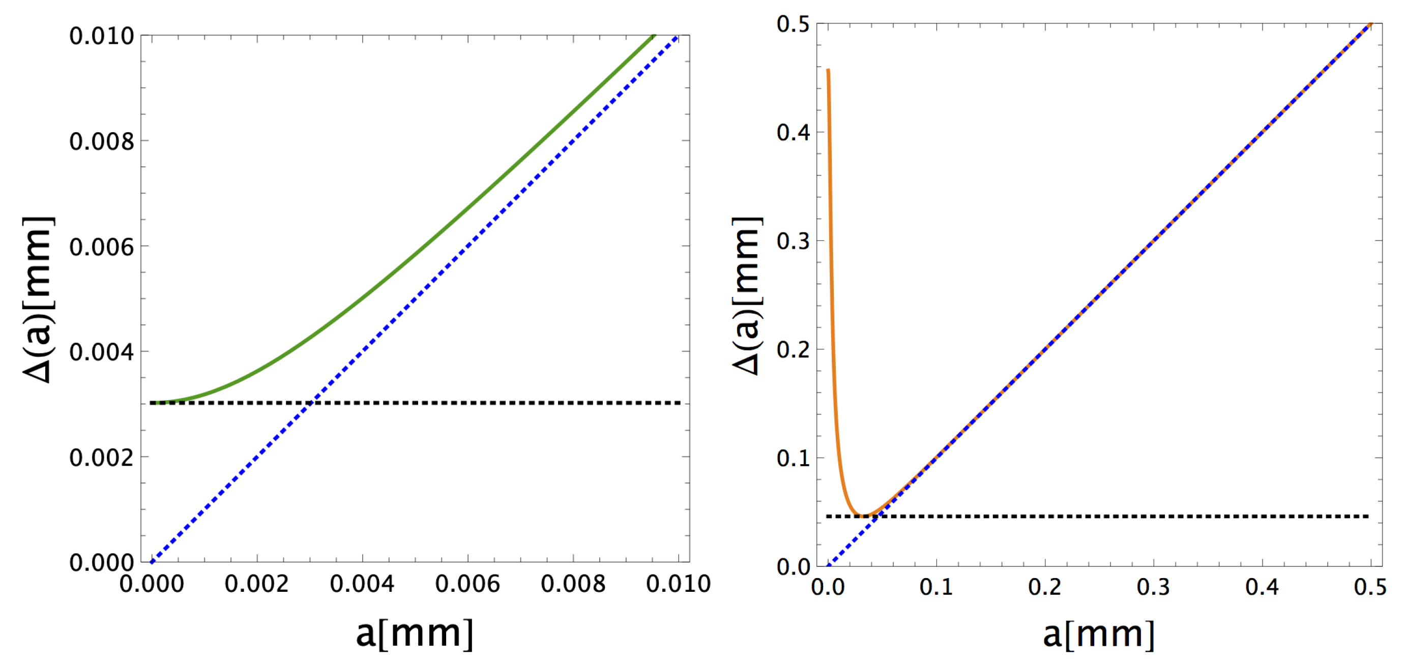
Figure 3.
Graphical identification of the width limit defined as in Equation (35), as the object width coinciding with the minimum of the total image width . The solid lines represent , while the dashed lines, corresponding to , are reported to show the onset of proportionality between image and object width. The horizontal dashed lines represent the minimum value of . The left panel represents the case , in which the object is placed in one of the two reference planes, focused on the detector, and is a constant. The right panel shows the case in which the object is placed midway between the two reference planes, namely in . Numerical values of the parameters are reported in the text.

Figure 4.
Behaviour of the limit object (dashed red line) and (solid blue line) as a function of the distance z between the object and the lens. The two functions have consistent behaviours, with minima close to the two reference planes and and a local maximum close to the midpoint . While the two limits coincide close to the focused planes, the limit is more restrictive by a factor of in out-of-focus cases.

Publisher’s Note: MDPI stays neutral with regard to jurisdictional claims in published maps and institutional affiliations. |
© 2022 by the authors. Licensee MDPI, Basel, Switzerland. This article is an open access article distributed under the terms and conditions of the Creative Commons Attribution (CC BY) license (https://creativecommons.org/licenses/by/4.0/).
Share and Cite
MDPI and ACS Style
Scattarella, F.; D’Angelo, M.; Pepe, F.V. Resolution Limit of Correlation Plenoptic Imaging between Arbitrary Planes. Optics 2022, 3, 138-149. https://0-doi-org.brum.beds.ac.uk/10.3390/opt3020015
AMA Style
Scattarella F, D’Angelo M, Pepe FV. Resolution Limit of Correlation Plenoptic Imaging between Arbitrary Planes. Optics. 2022; 3(2):138-149. https://0-doi-org.brum.beds.ac.uk/10.3390/opt3020015
Chicago/Turabian StyleScattarella, Francesco, Milena D’Angelo, and Francesco V. Pepe. 2022. "Resolution Limit of Correlation Plenoptic Imaging between Arbitrary Planes" Optics 3, no. 2: 138-149. https://0-doi-org.brum.beds.ac.uk/10.3390/opt3020015