Modelling of Irreversible Homogeneous Reaction on Finite Diffusion Layers

Abstract

The mathematical model proposed by Chapman and Antano (Electrochimica Acta, 56 (2010), 128–132) for the catalytic electrochemical–chemical (EC’) processes in an irreversible second-order homogeneous reaction in a microelectrode is discussed. The mass-transfer boundary layer neighbouring an electrode can contribute to the electrode’s measured AC impedance. This model can be used to analyse membrane-transport studies and other instances of ionic transport in semiconductors and other materials. Two efficient and easily accessible analytical techniques, AGM and DTM, were used to solve the steady-state non-linear diffusion equation’s infinite layers. Herein, we present the generalized approximate analytical solution for the solute, product, and reactant concentrations and current for the small experimental values of kinetic and diffusion parameters. Using the Matlab/Scilab program, we also derive the numerical solution to this problem. The comparison of the analytical and numerical/computational results reveals a satisfactory level of agreement.

1. Introduction

The role of electrochemical impedance spectroscopy in electrode processes is crucial. It is a useful experimental technique employed in an electrode procedure to categorise different mechanisms [1]. In the semi-infinite system, the diffusion-controlled resistance also contributes to the measured impedance. The phase at the electrode surface can have its diffusion impedance determined using the transport model [2,3,4,5,6]. Several authors [7,8,9,10,11] studied reactant diffusion through a stagnant diffusion layer of thickness. Juan Bisquert [12] discussed the theory of electron diffusion and recombination impedance in a thin layer. Ten years ago, Chapman and Antano [1] used a computational approach to find the approximate concentration profiles and impedance behaviour. Uma et al. [13] derived the approximate analytical expressions for the concentration of the system.

To the best of our knowledge, there is no concise and closed-form analytical equation provided for species concentrations in irreversible homogeneous reactions in finite-layer diffusion. This study intends to obtain new analytical expressions, in closed form, for the concentration of the reactant S, product P, and solute R for low values of the rate constant.

2. Mathematical Formulation

The following describes the reaction mechanism for a catalytic electrochemical system with diffusion and an irreversible second-order reaction in a stagnant diffusion layer [1]:

$$R\pm e^{-}\leftrightarrow P$$

(1)

$$P+S\stackrel{ k_2 }{\to }Y+R$$

(2)

The soluble substance P is produced at the electrode by the oxidation or reduction of the solute R. With the reaction rate constant, P reacts irreversibly in the solution to create the product Y and regenerate R from the electrochemically inactive reactant S that is already present in the bulk solution. Figure 1 depicts the overview of a second-order irreversible homogeneous reaction. The overall process involves the electrochemical conversion of S to Y, which is accelerated by R, with some accumulation of P, if the homogeneous reaction cannot completely utilise the material produced at the electrode. One particular example is the oxidation of sulfite (S) to sulphate (Y), which is accelerated by the ferrous ion (R) and results in the formation of a reactive ferric ion (P) at an anode.

Consider the non-linear differential equations [1] at steady-state conditions in a dimensionless form, as follows:

$$\frac{d^{2}R\left(x\right)}{d{x}^2}+k P\left(x\right) S\left(x\right)=0$$

(3)

$$\frac{d^{2}P\left(x\right)}{d{x}^2}-k P\left(x\right) S\left(x\right)=0$$

(4)

$$\frac{d^{2}S\left(x\right)}{d{x}^2}-k P\left(x\right) S\left(x\right)=0$$

(5)

where the dimensionless variables are

$$\begin{array}{c}R=\left[C_R/C_{Sb}\right],P=\left[C_P/C_{Sb}\right],S=\left[C_S/C_{Sb}\right],x=z/\delta \hfill \\ k=\left[k_2{C}_{Sb}/{\delta }^{2}D\right],\alpha =\left[C_{Rb}/C_{Sb}\right] \mathrm{and} \gamma =\left[C_{R0,SS}/C_{Sb}\right]\hfill \end{array}$$

(6)

where R, P, and S are the dimensionless concentrations solute, product, and the reactant, respectively; $x$ is the dimensionless distance. For simplicity, we have assumed that all three diffusion coefficients are equal to the value $D$; k is dimensionless rate constant. Two other parameters, $\alpha$ and $\gamma$, are the concentration ratios. The corresponding boundary conditions are as follows:

$$R=\gamma ;P=\alpha -\gamma ;\frac{dS}{dx}=0 \mathrm{when} x=0$$

(7)

$$R=\alpha ;P=0;S=1 \mathrm{when} x=1$$

(8)

where $\alpha >\gamma$. The non-dimensional current is given as

$$\psi =\frac{i\delta }{nFD{C}_{Sb}A}={\left|\frac{dR\left(x\right)}{dx}\right|}_{x=0}$$

(9)

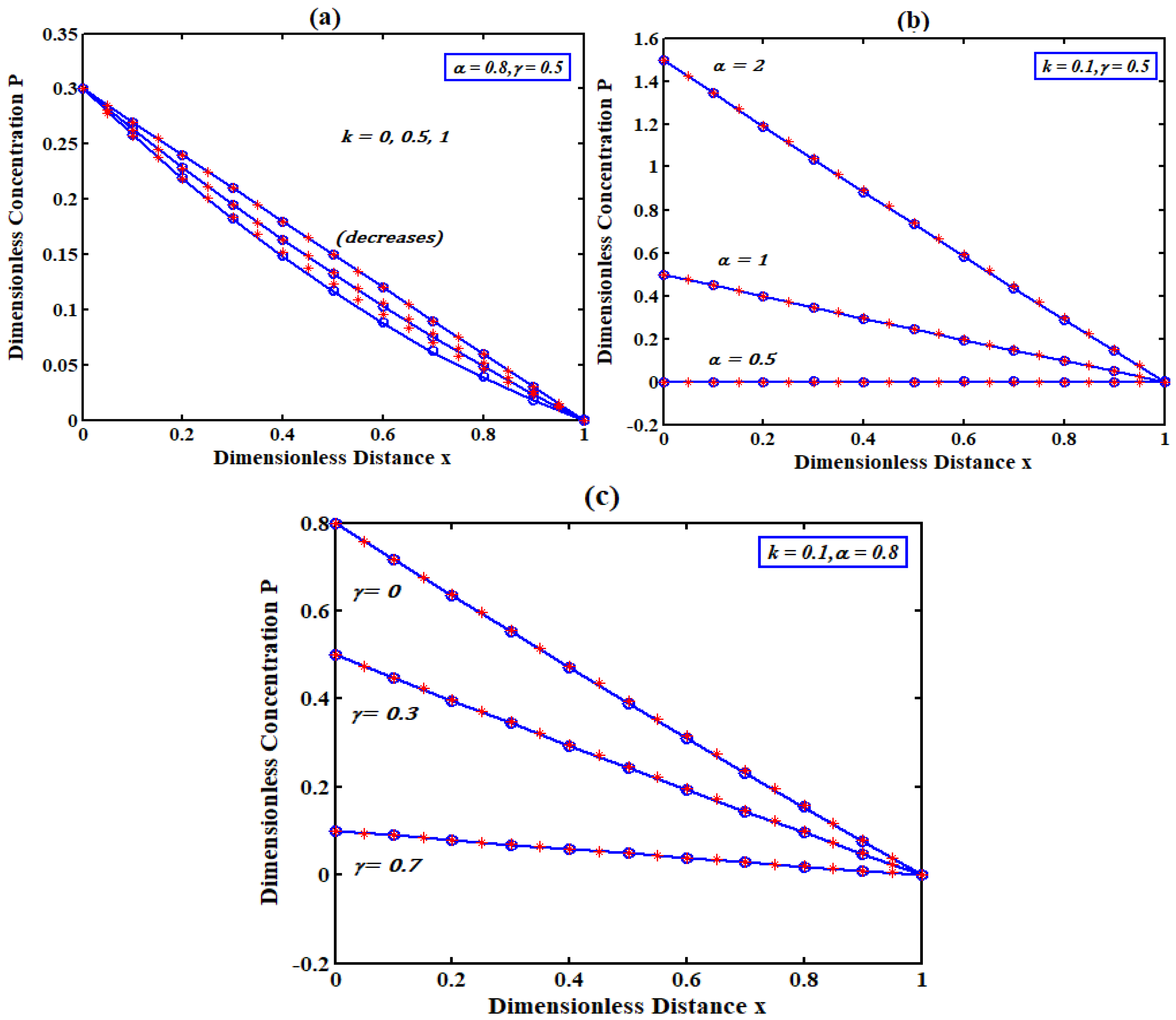
3. Analytical Expression of Concentrations

Equations (3)–(5) represent the nonlinear differential equations. Finding the precise solution to these nonlinear differential equations is difficult. One of the toughest challenges, especially across a wide range of science and engineering applications, is solving nonlinear differential equations. Recently, the construction of an analytical solution has been the focus of numerous analytical techniques, such as the homotopy perturbation method (HPM) [14,15,16,17,18,19,20,21,22,23,24,25,26], the variational iteration method [27,28,29,30,31,32], the homotopy analysis method [33,34,35,36,37], the Akbari-Ganji method [38,39,40,41,42,43], the Taylor series method [44,45,46,47], and the differential transform method. Jalili et al. [48,49,50] discussed the heat exchange in nano-particles and solved the momentum and energy equation numerically. In this paper, AGM and DTM are developed (Appendix A and Appendix B) for solving the ill-posted boundary value problem, which has the fewest number of unknowns, and its associated boundary conditions are represented by the Equations (3)–(8). For the nonlinear steady-state second-order equations, these are effective techniques.

3.1. Analytical Expression of Concentrations Using the Akbari-Ganji Method (AGM)

The Akbari-Ganji approach, created by the mathematicians Akbari and Ganji [38,39,40,41,42,43], is used in this study to solve the nonlinear differential equations governing this system. Moreover, with this method, we can quickly solve the nonlinear equations without any complex mathematical operations. The relation between the concentrations is given in Appendix A. Using this relationship and the proposed approach, the general analytical expression for normalized concentrations of the species are as follows (Appendix B):

$$R\left(x\right)=-\frac{cosh\left(mx\right)}{cosh\left(m\right)}+\left(\alpha +1\right) x-\left(\gamma +l\right)\left(x-1\right)$$

(10)

$$P\left(x\right)=\frac{cosh\left(mx\right)}{cosh\left(m\right)}-\left(\alpha +1\right) x+\left(\gamma +l\right)\left(x-1\right)+ \alpha$$

(11)

$$S\left(x\right)=\frac{cosh mx}{cosh m}$$

(12)

where the constant

$$m=\sqrt{k\left(\alpha -\gamma \right)}$$

(13)

Using Equation (7), the non-dimensional current is

$$=\frac{i\delta }{nFD{C}_{Sb}A}={\left|\frac{dR\left(x\right)}{dx}\right|}_{x=0}=1+\alpha -\gamma -sech\left(m\right)$$

(14)

3.2. Analytical Expression of Concentrations Using the Differential Transform Method (DTM)

A semi-analytical technique for resolving differential equations is the differential transform method (DTM). Zhou [35] was the first to put forth the differential transform idea, which is used to address both linear and nonlinear boundary value issues in electric circuit analysis. The nth derivative of an analytical function at a particular point can be precisely calculated using DTM, regardless of whether the boundary conditions are known or unknown. With this method, differential equations produce an empirical polynomial solution. This approach differs from the typical high-order Taylor series process, which requires the symbolic computation of the data functions. The Taylor series procedure takes some time to compute. The DTM is an alternative iterative procedure for obtaining analytical solutions of differential equations [36,37,38,39]. The approximate analytical expressions of concentrations using the DTM method are obtained as follows (Appendix C):

$$R\left(x\right)=\left(\alpha +1\right) x-\left(\gamma +\frac{2}{2+k\left(\alpha -\gamma \right)}\right)\left(x-1\right)-\frac{2+k \left(\alpha -\gamma \right)x^2}{2+k\left(\alpha -\gamma \right)}$$

(15)

$$P\left(x\right)=\alpha -\left(\alpha +1\right) x+\left(\gamma +\frac{2}{2+k\left(\alpha -\gamma \right)}\right)\left(x-1\right)+\frac{2+k \left(\alpha -\gamma \right)x^2}{2+k\left(\alpha -\gamma \right)}$$

(16)

$$S\left(x\right)=\frac{2+k \left(\alpha -\gamma \right)x^2}{2+k\left(\alpha -\gamma \right)}$$

(17)

4. Validation of Analytical Results with Numerical Simulation

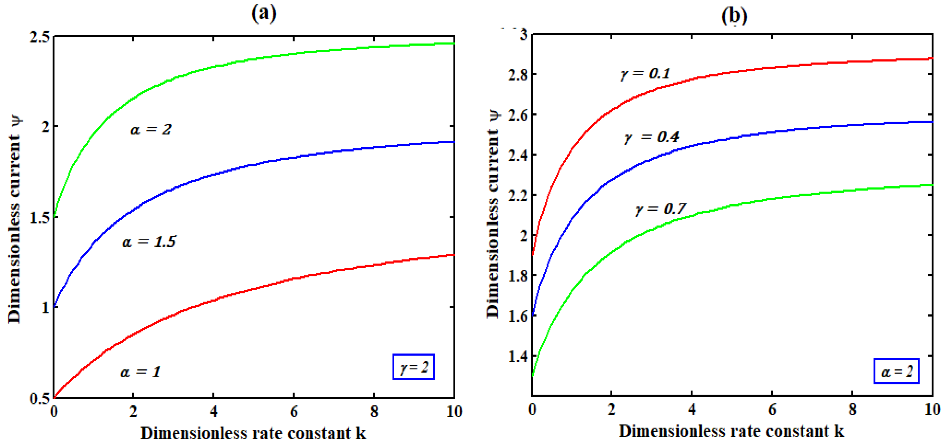
The validation method has received significant attention in the literature. Using the function pdex4 in the Scilab software, the nonlinear differential Equations (3)–(5), with the boundary conditions (7) and (8), are numerically solved. The Scilab code is also given in Appendix D. Figure 2 and Figure 3 compare the species concentrations obtained using the AGM technique, Equations (10)–(12), and the DTM method, Equations (15)–(17), with a numerical solution. Figure 4 represents the dimensionless current versus the dimensionless rate constant k.

Table 1. Comparison between the numerical and analytical expression of the concentration of the substrate obtained by AGM and DTM for the parameters $\alpha =0.8, \gamma =0.5,$ and for different values of k.

$\mathit{x}$	Substrate Concentration S
	$\mathit{k}=0$					$\mathit{k}=0.5$					$\mathit{k}=1$
	NUM	AGM Equation (12)	DTM Equation (17)	Error % for AGM	Error % for DTM	NUM	AGM Equation (12)	DTM Equation (17)	Error % for AGM	Error % for DTM	NUM	AGM Equation (12)	DTM Equation (17)	Error % for AGM	Error % for DTM
0	1	1	1	0	0	0.9535	0.9294	0.9302	2.53	2.44	0.913	0.8667	0.8696	5.07	4.75
0.25	1	1	1	0	0	0.9576	0.9338	0.9346	2.49	2.40	0.9206	0.8748	0.8777	4.98	4.66
0.5	1	1	1	0	0	0.9681	0.9469	0.9477	2.19	2.11	0.9405	0.8994	0.9022	4.37	4.07
0.75	1	1	1	0	0	0.9830	0.9689	0.9695	1.43	1.37	0.9683	0.9409	0.9429	2.83	2.62
1	1	1	1	0	0	1.0000	1.0000	1.0000	0.00	0.00	1.0000	1.0000	1.0000	0.00	0.00
	Average Error %			0	0	Average Error %			1.7274	1.6652	Average Error %			3.4481	3.2220

and

Table 2. Comparison between the numerical and analytical expression of the concentration of the substrate obtained by AGM and DTM for the parameters $k=0.1, \gamma =0.5,$ and for different values of $\alpha$.

$\mathit{x}$	Substrate Concentration S
	$\mathit{\alpha }=0.5$					$\mathit{\alpha }=1$					$\mathit{\alpha }=2$
	NUM	AGM Equation (12)	DTM Equation (17)	Error % for AGM	Error % for DTM	NUM	AGM Equation (12)	DTM Equation (17)	Error % for AGM	Error % for DTM	NUM	AGM Equation (12)	DTM Equation (17)	Error % for AGM	Error % for DTM
0	1	1	1	0	0	0.9837	0.9755	0.9756	0.83	0.82	0.9524	0.9294	0.9302	2.41	2.33
0.25	1	1	1	0	0	0.9851	0.9770	0.9771	0.82	0.81	0.9565	0.9338	0.9346	2.37	2.29
0.5	1	1	1	0	0	0.9888	0.9816	0.9817	0.73	0.72	0.9673	0.9469	0.9477	2.11	2.03
0.75	1	1	1	0	0	0.9940	0.9893	0.9893	0.47	0.47	0.9825	0.9689	0.9695	1.38	1.32
1	1	1	1	0	0	1.0000	1.0000	1.0000	0.00	0.00	1.0000	1.0000	1.0000	0.00	0.00
	Average Error %			0	0	Average Error %			0.5714	0.5653	Average Error %			1.6563	1.5940

NUM—numerical simulation; AGM—Akbari-Ganji method; DTM—differential transform method.

show the comparison between the numerical and analytical concentration of the substrate obtained by AGM and DTM for various values of parameters, α = 0.8, γ = 0.5, and for different values of k. From the tables it is found that the average relative errors are less than 5%. When considering the concentrations of the solute R, product P, and reactant S for small values of other parameters, our analytical results show satisfactory agreement for k ≤ 1.

5. Discussions

Equations (10)–(12) and (15)–(17) are the new simple analytical expressions of the concentrations of the solute R, product P, and the reactant S, respectively. The concentration profiles depend upon diffusion parameters (α and γ) and rate constant (k). In Figure 2a,c, the profile of the solute concentration is presented. These figures clearly show that for all small feasible values of the parameters, the solute concentration R increases at the electrode surfaces, whereas it drops as γ and k increase. Product concentration P increases in Figure 3a,c when the parameters k and alpha increase, while it increases when γ decreases. However, there is no discernible difference between the variances of the parameters k, α, and γ and the reactant concentration S. It has been noted that a rise in the rate constant k causes a fall in the S concentration. Figure 4a,b plots the current against parameter k. The figure indicates that the current increases as the rate constant k rises.

6. Conclusions

The set of nonlinear equations in the irreversible homogeneous reaction for finite diffusion is discussed in this study. Common analytical expressions are provided for the concentration of solute, product, reactant, and current for all diffusion values and the small values of the kinetic parameters. Compared with other analytical methods, the AGM and DTM are straightforward, with a simple solution processes, yielding accurate results. The non-steady-state circumstances can also be handled with these methods. The theoretical and numerical results were further contrasted, and they were found to be in good accord. The method described here can be applied to examine membrane-transport studies, as well as some other instances of ionic transport in semi-conductors and solid electrolytes. This theoretical approach could be applied in more complicated cases when the transport equation contains non-linearities. It can also be used with membranes and solid electrolytes, where diffusion is a crucial phenomenon.

References

1. Thomas, W.; Chapman, T.W.; Antano, R. The effect of an irreversible homogeneous reaction on finite-layer diffusion impedance. Electrochim. Acta 2010, 56, 128. [Google Scholar]
2. Orazem, M.E.; Tribollet, B. Electrochemical Impedance Spectroscopy, Theory; John Wiley and Sons Inc.: Hoboken, NJ, USA, 2008. [Google Scholar]
3. Lasia, A. Electrochemical Impedance Spectroscopy and its applications. In Modern Aspects of Electrochemistry; Conway, B.E., Bockris, J.O.M., White, R.E., Eds.; Plenum Press: New York, NY, USA, 1999; Volume 32, p. 143. [Google Scholar]
4. Lasia, A. Applications of Electrochemical Impedance Spectroscopy to Hydrogen Adsorption, Evolution and Absorption into Metals. In Modern Aspects of Electrochemistry; Conway, B.E., White, R.E., Eds.; Kluwer Springer: New York, NY, USA, 2002; Volume 35, p. 1. [Google Scholar]
5. Montella, C. Review and theoretical analysis of ac–av methods for the investigation of hydrogen insertion I. Diffusion formalism. J. Electroanal. Chem. 1999, 462, 73. [Google Scholar] [CrossRef]
6. Montella, C. Review and theoretical analysis of ac–av methods for the investigation of hydrogen insertion: Part III. Comparison of entry side impedance, transfer function and transfer impedance methods. J. Electroanal. Chem. 2000, 480, 150. [Google Scholar] [CrossRef]
7. Drossbach, P.; Schultz, J. Elektrochemischeuntersuchungen an kohleelektroden—I: Die überspannung des wasserstoffs. Electrochim. Acta 1964, 9, 1391. [Google Scholar] [CrossRef]
8. Franceschetti, D.R.; Macdonald, J.R.; Buck, R.P. Interpretation of finite-length-warburg-type impedances in supported and unsupported electrochemical cells with kinetically reversible electrodes. J. Electrochem. Soc. 1991, 138, 1368. [Google Scholar] [CrossRef]
9. Diard, J.P.; le Gorrec, B.; Montella, C. Linear diffusion impedance. General expression and applications. J. Electroanal. Chem. 1999, 471, 126. [Google Scholar] [CrossRef]
10. Franceschetti, D.R.; Macdonald, J.R. Diffusion of neutral and charged species under small-signal a.c. conditions. J. Electroanal. Chem. 1979, 101, 307. [Google Scholar] [CrossRef]
11. Macdonald, J.R. Impedance Spectroscopy, Emphasizing Solid Materials and Systems, Theory; John Wiley and Sons Inc.: New York, NY, USA, 1987; p. 45. [Google Scholar]
12. Bisquert, J. Theory of the impedance of electron diffusion and recombination in a thin layer. J. Phys. Chem. B 2002, 106, 325. [Google Scholar] [CrossRef]
13. Maheswari, M.U.; Rajendran, L. Analytical expressions of concentrations of substrate and hydroquinone in an amperometric glucose biosensor. Int. Sch. Res. Not. 2012, 3, 2089. [Google Scholar] [CrossRef]
14. Vijayalakshmi, T.; Senthamarai, R. Analytical approach to a three species food chain model by applying homotopy perturbation method. Int. J. Adv. Sci. Technol. 2020, 29, 2853. [Google Scholar]
15. Umadevi, R.; Venugopal, K.; Jeyabarathi, P.; Rajendran, L.; Abukhaled, M. Analytical study of nonlinear roll motion of ships: A homotopy perturbation approach. Palest. J. Math. 2022, 11, 316. [Google Scholar]
16. Manimegalai, B.; Lyons, M.E.G.; Rajendran, L. Transient chronoamperometric current at rotating disc electrode for second-order ECE reactions. J. Electroanal. Chem. 2021, 902, 115775. [Google Scholar] [CrossRef]
17. Salomi, R.J.; Sylvia, S.V.; Rajendran, L.; Lyons, M.E.G. Lyons, Transient current, sensitivity and resistance of biosensors acting in a trigger mode: Theoretical study. J. Electroanal. Chem. 2021, 895, 115421. [Google Scholar] [CrossRef]
18. Manimegalai, B.; Rajendran, L.; Lyons, M.E.G. Theory of the transient current response for the homogeneous mediated enzyme catalytic mechanism at the rotating disc electrode. Int. J. Electrochem. Sci. 2021, 16, 41. [Google Scholar] [CrossRef]
19. Swaminathan, R.; Saravanakumar, R.; Venugopal, K.; Rajendran, L. Analytical solution of non linear problems in homogeneous reactions occur in the mass-transfer boundary layer: Homotopy Perturbation Method. Int. J. Electrochem. Sci. 2021, 16, 115421. [Google Scholar] [CrossRef]
20. He, J.H. Homotopy perturbation technique. Comput. Methods Appl. Mech. Eng. 1999, 178, 257. [Google Scholar] [CrossRef]
21. He, J.H. A coupling method of a homotopy technique and a perturbation technique for non-linear problems. Int. J. Nonlinear Mech. 2000, 35, 37. [Google Scholar] [CrossRef]
22. Saravanakumar, R.; Pirabaharan, P.; Abukhaled, M.; Rajendran, L. Theoretical analysis of voltammetry at a rotating disk electrode in the absence of supporting electrolyte. J. Phys. Chem. B 2020, 124, 443. [Google Scholar] [CrossRef]
23. He, J.H. Variational iteration method for autonomous ordinary differential systems. Appl. Math. Comput. 2000, 114, 115. [Google Scholar] [CrossRef]
24. Odibat, Z.; Momani, S. A generalized differential transform method for linear partial differential equations of fractional order. Appl. Math. Lett. 2008, 21, 194. [Google Scholar] [CrossRef]
25. Saranya, K.; Mohan, V.; Rajendran, L. Steady-state concentrations of carbon dioxide absorbed into phenyl glycidyl ether solutions by residual method. J. Math. Chem. 2020, 58, 1230. [Google Scholar] [CrossRef]
26. Nirmala, K.; Manimegalai, B.; Rajendran, L. Steady-State substrate and product concentrations for non michaelis-menten kinetics in an amperometric biosensor–hyperbolic function and Padé approximants method. Int. J. Electrochem. Sci. 2020, 15, 5682. [Google Scholar] [CrossRef]
27. Mallikarjuna, M.; Senthamarai, R. Analytical solution of enzyme catalysis in calcium alginate. In Proceedings of the 6th International Conference on Materials Technology and Applications (ICMTA 2021) AIPCP22-AR-ICMTA, Fukuoka, Japan, 30 October–2 November 2021. [Google Scholar]
28. Rajendran, L.; Rahamathunissa, G. Application of He’s variational iteration method in nonlinear boundary value problems in enzyme–substrate reaction diffusion processes: Part 1. The steady-state amperometric response. J. Math. Chem. 2008, 44, 849. [Google Scholar]
29. Eswari, A.; Rajendran, L. Application of variational iteration method and electron transfer mediator/catalyst composites in modified electrodes. Nat. Sci. 2010, 2, 612. [Google Scholar] [CrossRef] [Green Version]
30. Loghambal, S.; Rajendran, L. Analysis of amperometric enzyme electrodes in the homogeneous mediated mechanism using variational iteration method. Int. J. Electrochem. Sci. 2010, 5, 327. [Google Scholar]
31. Devi, M.R.; Rajendran, L. A new mathematical modelling using homotopy perturbation method to solve nonlinear equations in enzymatic glucose fuel cells. Int. J. Math. Arch. 2014, 5, 142. [Google Scholar]
32. Ibrahim, M.S.; Pavithra, S.; Saravanakumar, R.; Ashokan, R.; Rajendran, L. Modelling of Non Linear Enzyme Reaction Process Using Variational Iteration Method. Int. J. Comp. Eng. Res. 2016, 6, 2250. [Google Scholar]
33. Suganya, G.; Senthamarai, R. Mathematical modeling and analysis of the effect of the rugose spiraling whitefly on coconut trees. AIMS Math. 2022, 7, 13053. [Google Scholar]
34. Adomian, G. A review of the decomposition method in applied mathematics. J. Math. Anal. Appl. 1988, 135, 501. [Google Scholar] [CrossRef]
35. Liao, S.J. A kind of approximate solution technique which does not depend upon small parameters (II): An application in fluid mechanics. Int. J. Nonlinear Mech. 1997, 32, 815. [Google Scholar] [CrossRef]
36. Liao, S.J. Homotopy analysis method for heat radiation equations. Appl. Math. Comput. 2007, 147, 499. [Google Scholar]
37. Liao, S.J. Comparison between the homotopy analysis method and homotopy perturbation method. Appl. Math. Comput. 2005, 169, 1186. [Google Scholar] [CrossRef]
38. Akbari, M.R.; Ganji, D.D.; Nimafar, M.; Ahmadi, A.R. Significant progress in solution of nonlinear equations at displacement of structure and heat transfer extended surface by new AGM approach. Front. Mech. Eng. 2014, 9, 390–401. [Google Scholar] [CrossRef]
39. Pirabaharan, P.; Devi, M.C.; Swaminathan, R.; Rajendran, L.; Lyons, M.E.G. Modelling the current response and sensitivity of oxidase enzyme electrodes, Monitored Amperometrically by the Consumption of Oxygen. Electrochem 2022, 3, 309–321. [Google Scholar] [CrossRef]
40. Shanthi, R.; Devi, M.C.; Abukhaled, M.; Lyons, M.E.G.; Rajendran, L. Mathematical modeling of ph-based potentiometric biosensor using Akbari-Ganji method. Int. J. Electrochem. Sci. 2022, 17, 2. [Google Scholar] [CrossRef]
41. Padma, S.; Jeyabarathi, P.; Rajendran, L.; Lyons, M.E.G. A kinetic model for amperometric immobilized enzymes at planar, cylindrical and spherical electrodes: The Akbari-Ganji Method. Int. J. Electrochem. Sci. 2022, 17, 114921. [Google Scholar]
42. Manimegalai, B.; Lyons, M.E.; Rajendran, L. Mathematical modeling of substrate consumption in a biofilm: Solutions arrived using Akbari-Ganji method. J. Electroanal. Chem. 2021, 880, 114921. [Google Scholar] [CrossRef]
43. Vanaja, R.; Jeyabarathi, P.; Rajendran, L.; Lyons, M.E.G. The Analytical Expression of Steady-State Concentration of Mixture of Toluene and N- Propanol in the Biofilm: Akbari-Ganji’s method. Int. J. Electrochem. Sci. 2022, 17, 2. [Google Scholar] [CrossRef]
44. Sivasundari, S.A.S.; Rani, R.U.; Lyons, M.E.G.; Rajendran, L. Transport and Kinetics in Biofiltration Membranes: New analytical expressions for concentration profiles of hydrophilic and hydrophobic VOCs Using Taylor’s Series and Akbari-Ganji methods. Int. J. Electrochem. Sci. 2022, 17, 2. [Google Scholar]
45. Umadevi, R.; Devi, M.C.; Venugopal, K.; Rajendran, L.; Lyons, M.E. Theoretical analysis of reaction-diffusion process in biocatalyst modified electrodes: Solutions derived via Akbari-Ganji method and Taylor’s series with Ancient Chinese algorithms. Int. J. Electrochem. Sci. 2022, 17, 2. [Google Scholar] [CrossRef]
46. Lilly Clarance Mary, M.; Chitra Devi, M.; Meena, A.; Rajendran, L.; Abukhaled, M. A reliable Taylor series solution to the nonlinear reaction-diffusion model representing the steady-state behaviour of a cationic glucose-sensitive membrane. J. Math. Comput. Sci. 2021, 11, 8354. [Google Scholar]
47. Vinolyn Sylvia, S.; Joy Salomi, R.; Rajendran, L.; Abukhaled, M. Solving nonlinear reaction–diffusion problem in electrostatic interaction with reaction-generated pH change on the kinetics of immobilized enzyme systems using Taylor series method. J. Math. Chem. 2021, 59, 1332. [Google Scholar] [CrossRef]
48. Jalili, B.; Aghaee, N.; Jalili, P.; Ganji, D.D. Novel usage of the curved rectangular fin on the heat transfer of a double-pipe heat exchanger with a nanofluid. Case Stud. Therm. Eng. 2022, 35, 102086. [Google Scholar] [CrossRef]
49. Jalili, B.; Ghafoori, H.; Jalili, P. Investigation of carbon nano-tube (CNT) particles effect on the performance of a refrigeration cycle. Int. J. Mater. Sci. Innov. 2014, 2, 8–17. [Google Scholar]
50. Jalili, P.; Kazerani, K.; Jalili, B.; Ganji, D.D. Investigation of thermal analysis and pressure drop in non-continuous helical baffle with different helix angles and hybrid nano-particles. Case Stud. Therm. Eng. 2022, 36, 102209. [Google Scholar] [CrossRef]
Figure 1. General scheme of a second-order irreversible homogeneous reaction.
Electrochem 03 00033 g001
Figure 2. (ac) Profile of the normalized steady-state concentrations R versus the normalized distance x for various values of the parameters k ,   α ,   and   γ   using Equations (10) and (15) The solid line denotes the AGM method, (o o o) represents DTM, and (* * *) denotes numerical simulation.
Electrochem 03 00033 g002aElectrochem 03 00033 g002b
Figure 3. (ac): Profile of the normalized steady-state concentrations P versus the normalized distance x for various values of the parameters k ,   α , and γ using Equations (11) and (16). The solid line denotes the AGM method, (o o o) represents DTM, and (* * *) denotes numerical simulation.
Electrochem 03 00033 g003
Figure 4. (a,b): Dimensionless current versus dimensionless rate constant k .
Electrochem 03 00033 g004