
Revisiting the Lognormal Modelling of Shadowing Effects during Wireless Communications by Means of the α-μ/α-μ Composite Distribution


Abstract
:1. Introduction
2. The - Distribution
Mathematical Definitions
3. Composite Fading Model
Simplified Results When
4. Numerical Evaluation of the Expressions
4.1. Integral Representations
4.2. Series Representations
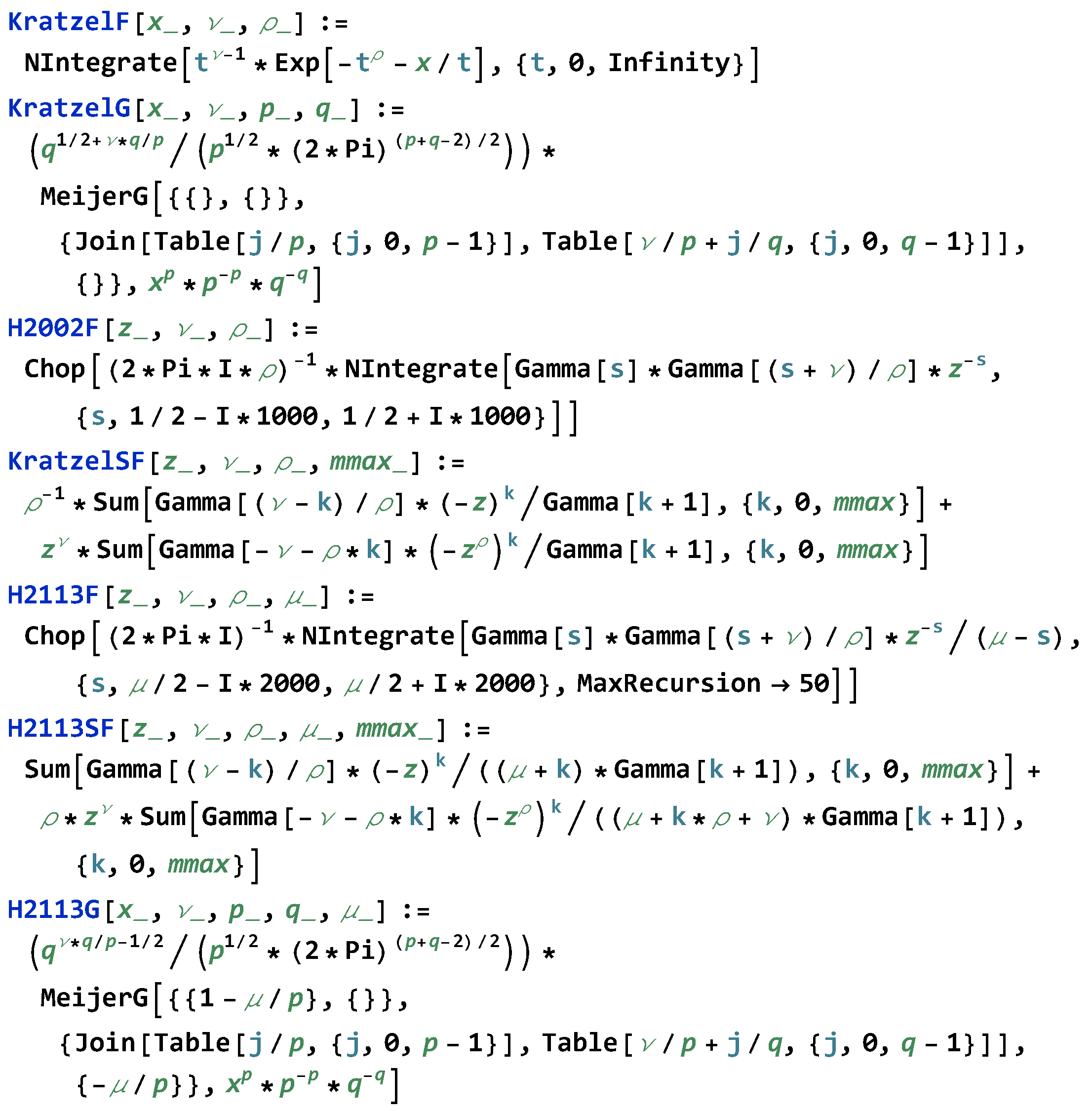
- The function implements the numerical integral definition of the Kratzel function given right below (5).
- implements the Meijer G-function alternative representation of the Kratzel function used to obtain (9) whenever .
- implements the H-function alternative definition of the Kratzel function used to obtain (6).
- implements the series representation of the Kratzel function given in (11). Here, represents the number of terms to be considered for the summation.
- implements the H-function used in (7).
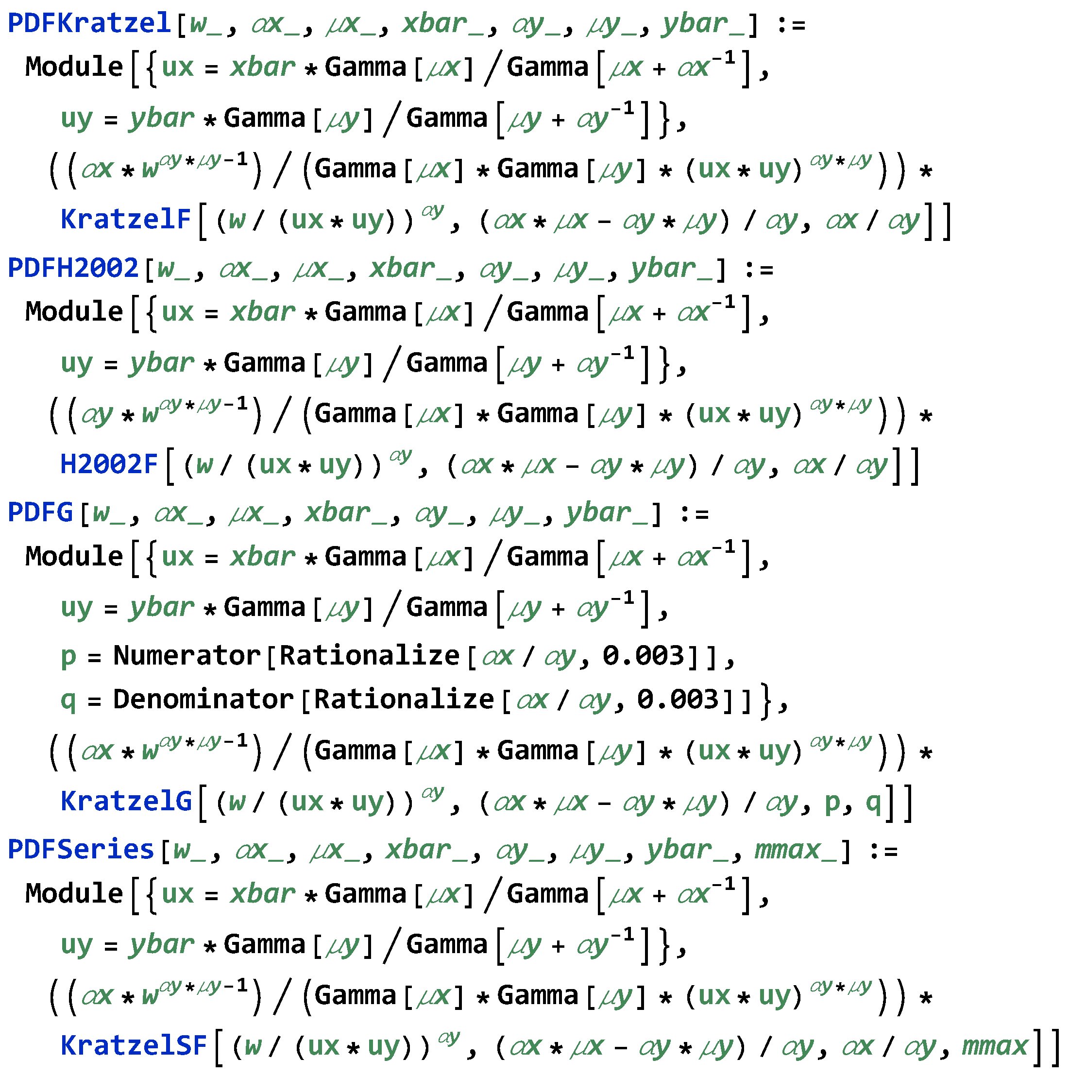
- The function implements the PDF of the composed distribution when the numerical integral definition of the Kratzel function is used.
- implements the PDF of the composed distribution when the H-function alternative definition of the Kratzel function is used.
- implements the PDF of the composed distribution when and the Meijer G-function alternative definition of the Kratzel function is used. In order to obtain the rational approximations to , we automatically calculate the rational number with smallest denominator that lies within of the real ratio.
- implements the series expression of the PDF by considering terms into the summation.
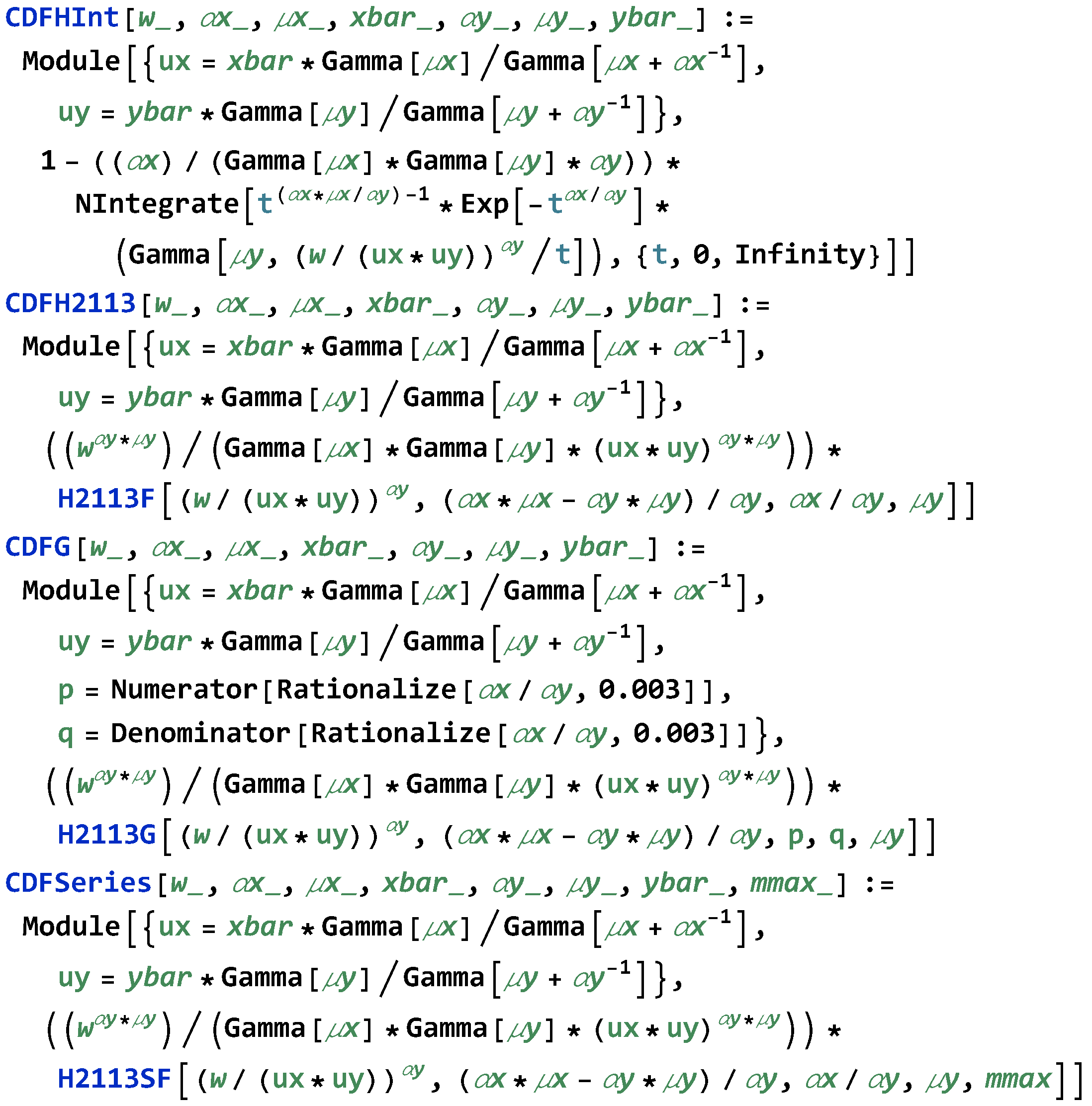
- The function implements the CDF of the composed distribution when the numerical integral definition of the Kratzel function is used.
- implements the CDF of the composed distribution when the numerical integral definition of the H-function is used.
- implements the CDF of the composed distribution when and the Meijer G-function alternative definition of the Kratzel function is used. In order to obtain the rational approximations to , we automatically calculate the rational number with smallest denominator that lies within of the real ratio.
- implements the series expression of the CDF by considering terms into the summation.
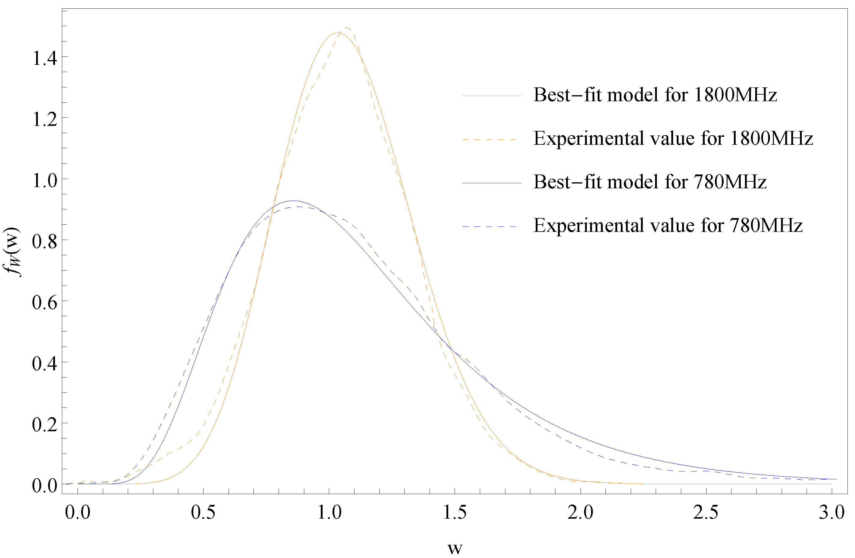
5. Application to Experimental Data
6. Conclusions
Author Contributions
Funding
Institutional Review Board Statement
Informed Consent Statement
Data Availability Statement
Acknowledgments
Conflicts of Interest
References
- Leonardo, E.J.; Yacoub, M.D. The Product of Two α-μ Variates and the Composite α-μ Multipath-Shadowing Model. IEEE Trans. Veh. Technol. 2015, 64, 2720–2725. [Google Scholar] [CrossRef]
- Suzuki, H. A statistical model for urban radio propagation. IEEE Trans. Commun. 1977, 25, 673–680. [Google Scholar] [CrossRef]
- Hansen, F.; Meno, F.I. Mobile fading Rayleigh and lognormal superimposed. IEEE Trans. Veh. Technol. 1977, 26, 332–335. [Google Scholar] [CrossRef]
- Abu-Dayya, A.A.; Beaulieu, N.C. Micro- and macrodiversity NCFSK (DPSK) on shadowed Nakagami-fading channels. IEEE Trans. Commun. 1994, 42, 2693–2702. [Google Scholar] [CrossRef]
- Abdi, A.; Kaveh, M. On the utility of gamma pdf in modeling shadow fading (slow fading). In Proceedings of the 1999 IEEE 49th Vehicular Technology Conference, Houston, TX, USA, 16–20 May 1999. [Google Scholar]
- Silva, W.A.; Mota, K.M.; Dias, U.S. Spectrum Sensing over Nakagami-m/Gamma Composite Fading Channel with Noise Uncertainty. In Proceedings of the 2015 IEEE Radio and Wireless Symposium (RWS), San Diego, CA, USA, 25–28 January 2015. [Google Scholar]
- Agrawal, R. On Efficacy of Rayleigh-Inverse Gaussian Distribution over K-distribution for Wireless Fading Channels. Wirel. Commun. Mob. Comput. 2007, 7, 1–7. [Google Scholar] [CrossRef]
- Chauhan, P.S.; Tiwari, D.; Soni, S.K. New analytical expressions for the performance metrics of wireless communication system over Weibull/Lognormal composite fading. AEU Int. J. Electron. Commun. 2017, 82, 397–405. [Google Scholar] [CrossRef]
- Mota, K.M.; Silva, W.A.; Ozelim, L.C.S.M.; Vale, L.M.; Dias, U.S.; Rathie, P.N. Spectrum sharing systems capacity under η–μ fading environments. J. Frankl. Inst. 2019, 356, 6741–6756. [Google Scholar] [CrossRef]
- Yacoub, M.D. The α-μ distribution: A physical fading model for the Stacy distribution. IEEE Trans. Veh. Technol. 2007, 56, 27–34. [Google Scholar] [CrossRef]
- Alvi, S.H.; Wyne, S.; da Costa, D.B. Performance analysis of dual-hop AF relaying over α-μ—Fading channels. AEU Int. J. Electron. Commun. 2019, 108, 221–225. [Google Scholar] [CrossRef]
- Dias, U.S.; Yacoub, M.D. On the α-μ Autocorrelation and Power Spectrum Functions: Field Trials and Validation. In Proceedings of the GLOBECOM 2009—2009 IEEE Global Telecommunications Conference, Honolulu, HI, USA, 30 November–4 December 2009; pp. 1–6. [Google Scholar]
- Reig, J.; Rubio, L. Estimation of the Composite Fast Fading and Shadowing Distribution Using the Log-Moments in Wireless Communications. IEEE Trans. Wirel. Commun. 2013, 12, 3672–3681. [Google Scholar] [CrossRef]
- Badarneh, O. The α-μ/α-μ composite multipath-shadowing distribution and its connection with the extended generalized-K distribution. AEU Int. J. Electron. Commun. 2016, 70, 1211–1218. [Google Scholar] [CrossRef]
- Samimi, H. Performance analysis of lognormally shadowed generalized Gamma fading channels. J. Commun. Syst. 2011, 24, 14–26. [Google Scholar] [CrossRef]
- Lawless, J.F. Statistical Models Furthermore, Methods for Lifetime Data; John Wiley & Sons, Inc.: New York, NY, USA, 2002. [Google Scholar]
- Kilbas, A.; Saxena, R.K.; Trujillo, J. Kratzel Function as a Function of Hypergeometric Type. Fract. Calc. Appl. Anal. 2006, 9, 109–131. [Google Scholar]
- Mathai, A.M.; Haubold, H.J. Special Functions for Applied Scientist; Springer: New York, NY, USA, 2008. [Google Scholar]
- Chauhan, P.S.; Kumar, S.; Soni, S.K. New approximate expressions of average symbol error probability, probability of detection and AUC with MRC over generic and composite fading channels. AEU Int. J. Electron. Commun. 2019, 99, 119–129. [Google Scholar] [CrossRef]
- Kumar, S.; Chauhan, P.S.; Raghuwanshi, P.; Kaur, M. ED performance over α-η-μ/IG and α-κ-μ/IG generalized fading channels with diversity reception and cooperative sensing: A unified approach. AEU Int. J. Electron. Commun. 2018, 97, 273–279. [Google Scholar] [CrossRef]
- Piretti, S.P.; Bretas, P.C.B., Jr.; Dias, U.S. On the α-μ/Gamma Composite Distribution: Field Trials and Validation. In Proceedings of the XXXI Simpósio Brasileiro de Telecomunicações (SBrT 2013), Fortaleza, Brazil, 17–19 September 2013. [Google Scholar]


| Set | |||
|---|---|---|---|
| S1 | |||
| S2 | |||
| S3 | |||
| S4 |
| (a) Equation (12) | ||||
| Set | Exact Value | 10 Terms | 30 Terms | 100 Terms |
| S1 | 0.207465 | 0.204785 | 0.207465 | 0.207465 |
| S2 | 0.127178 | 0.127178 | 0.127178 | 0.127178 |
| S3 | 0.126769 | 0.275901 | 0.126769 | 0.126769 |
| S4* | 0.383627 | 0.391774 | 0.391728 | |
| (b) Equation (13) | ||||
| Set | Exact Value | 10 Terms | 30 Terms | 100 Terms |
| S1 | 0.130012 | 0.129598 | 0.130012 | 0.130012 |
| S2 | 0.0926511 | 0.0926511 | 0.0926511 | 0.0926511 |
| S3 | 0.959844 | 0.96768 | 0.959844 | 0.959844 |
| S4* | 0.248891 | 0.272829 | 0.272827 | |
Publisher’s Note: MDPI stays neutral with regard to jurisdictional claims in published maps and institutional affiliations. |
© 2021 by the authors. Licensee MDPI, Basel, Switzerland. This article is an open access article distributed under the terms and conditions of the Creative Commons Attribution (CC BY) license (http://creativecommons.org/licenses/by/4.0/).
Share and Cite
Ozelim, L.C.S.M.; Dias, U.S.; Rathie, P.N. Revisiting the Lognormal Modelling of Shadowing Effects during Wireless Communications by Means of the α-μ/α-μ Composite Distribution. Modelling 2021, 2, 197-209. https://0-doi-org.brum.beds.ac.uk/10.3390/modelling2020010
Ozelim LCSM, Dias US, Rathie PN. Revisiting the Lognormal Modelling of Shadowing Effects during Wireless Communications by Means of the α-μ/α-μ Composite Distribution. Modelling. 2021; 2(2):197-209. https://0-doi-org.brum.beds.ac.uk/10.3390/modelling2020010
Chicago/Turabian StyleOzelim, Luan C. S. M., Ugo S. Dias, and Pushpa N. Rathie. 2021. "Revisiting the Lognormal Modelling of Shadowing Effects during Wireless Communications by Means of the α-μ/α-μ Composite Distribution" Modelling 2, no. 2: 197-209. https://0-doi-org.brum.beds.ac.uk/10.3390/modelling2020010