
A Tutorial on Fire Domino Effect Modeling Using Bayesian Networks


School of Occupational and Public Health, Ryerson University, Toronto, ON M5B 1Z5, Canada
Modelling 2021, 2(2), 240-258; https://0-doi-org.brum.beds.ac.uk/10.3390/modelling2020013
Submission received: 7 March 2021
/
Revised: 15 April 2021
/
Accepted: 19 April 2021
/
Published: 22 April 2021
Abstract
:High complexity and growing interdependencies of chemical and process facilities have made them increasingly vulnerable to domino effects. Domino effects, particularly fire dominoes, are spatial-temporal phenomena where not only the location of involved units, but also their temporal entailment in the accident chain matter. Spatial-temporal dependencies and uncertainties prevailing during domino effects, arising mainly from possible synergistic effects and randomness of potential events, restrict the use of conventional risk assessment techniques such as fault tree and event tree. Bayesian networks—a type of probabilistic network for reasoning under uncertainty—have proven to be a reliable and robust technique for the modeling and risk assessment of domino effects. In the present study, applications of Bayesian networks to modeling and safety assessment of domino effects in petroleum tank terminals has been demonstrated via some examples. The tutorial starts by illustrating the inefficacy of event tree analysis in domino effect modeling and then discusses the capabilities of Bayesian network and its derivatives such as dynamic Bayesian network and influence diagram. It is also discussed how noisy OR can be used to significantly reduce the complexity and number of conditional probabilities required for model establishment.
1. Introduction
1.1. Approaches to Domino Effect Modeling
Domino effects are low probability, high-consequence events the modeling and safety assessment of which are challenging due to their uncertainty and complexity. The uncertainty in the modeling and analysis of domino effects is partly due to the rarity of domino effects and thus the insufficiency of data required for their quantitative assessments. And partly due to the randomness of potential events during domino effects, including the synergistic effects and mutual impact of events. Therefore, modeling of domino effects has been conducted largely under oversimplifying assumptions and by admitting high uncertainty of the outcomes [1,2]. Methods developed for domino effect modeling and risk assessment can generally be divided into analytical models, numerical models, and graphic models [2].
Analytical models [3,4,5,6,7,8,9] have been based on the prediction of escalation probabilities based on analytical relationships between heat flux and vulnerability of exposed units. Despite being simple and computationally affordable, the analytical models usually suffer from oversimplified assumptions, and most of them cannot seem to recognize the possibility of high-order domino effects or synergistic effects. This shortcoming not only may give rise to an underestimation of the potential risk but may lead to improper allocation of safety measures [2,10].
Numerical modeling of fire and explosion [11,12,13,14,15] have greatly improved the accuracy of calculated heat fluxes and respective failure probability of exposed units. The past numerical studies of domino effects, which have mostly been based on applications of computational fluid dynamics (CFD) software such as Fire Dynamics Simulator are computationally expensive and resource-demanding, limiting their applications only to very simple chemical facilities in terms of layout and variety of process units. Due to their deterministic syntax, numerical models should be combined with probabilistic techniques to cope with uncertainty embedded in the variables and escalation scenarios.
Graphic models have become very popular in recent years in modeling and analysis of domino effects mainly due to their structures, which can closely represent domino effects (the units of a chemical facility as the nodes of the graph and the escalation vectors as the arcs of the graph). That most graphic models are probabilistic is a bonus in modeling domino effects where uncertainties play a key role in estimating the escalation probabilities and scenarios. Approaches based on event tree [16,17], Bayesian network (BN) [10,18], event sequence diagram [19], Petri net [20,21], and graph metrics [22,23,24]. Among these graphic techniques, BN has proved as a robust technique for modeling domino effects due to its ability in considering uncertainties (as opposed to graph metrics), considering interdependencies and nonlinear interactions (as opposed to event tree) and performing probability updating (as opposed to Petri net). In the next section, the modeling advantages of BN over a conventional technique-event tree–are demonstrated via an example.
1.2. Bayesian Network vs. Conventional Techniques
To make the discussion more concrete, consider three fuel storage tanks T1, T2, and T3, where a tank fire at T1 as a primary event can spread to T2, T3, or both, leading to a domino effect (Figure 1). In that case, three different domino scenarios could be envisaged:
- (1)
- The fire spreads from T1 to T2 (a level 1 domino effect: T1→T2). The heat fluxes radiating from fires at T1 and T2 can superimpose (known as synergistic effect) to cause damage to T3 and have the fire spread to it, resulting in a level 2 domino effect: T1→T2→T3.
- (2)
- The fire spreads from T1 to T3 (a level 1 domino effect: T1→T3). The heat fluxes radiating from fires at T1 and T3 may superimpose to cause damage to T2 via synergistic effect and have the fire spread to T2, resulting in a level 2 domino effect: T1→T3→T2.
- (3)
- The fire spreads from T1 to both T2 and T3 almost simultaneously, resulting in a level 1 domino effect: T1→T2 & T3
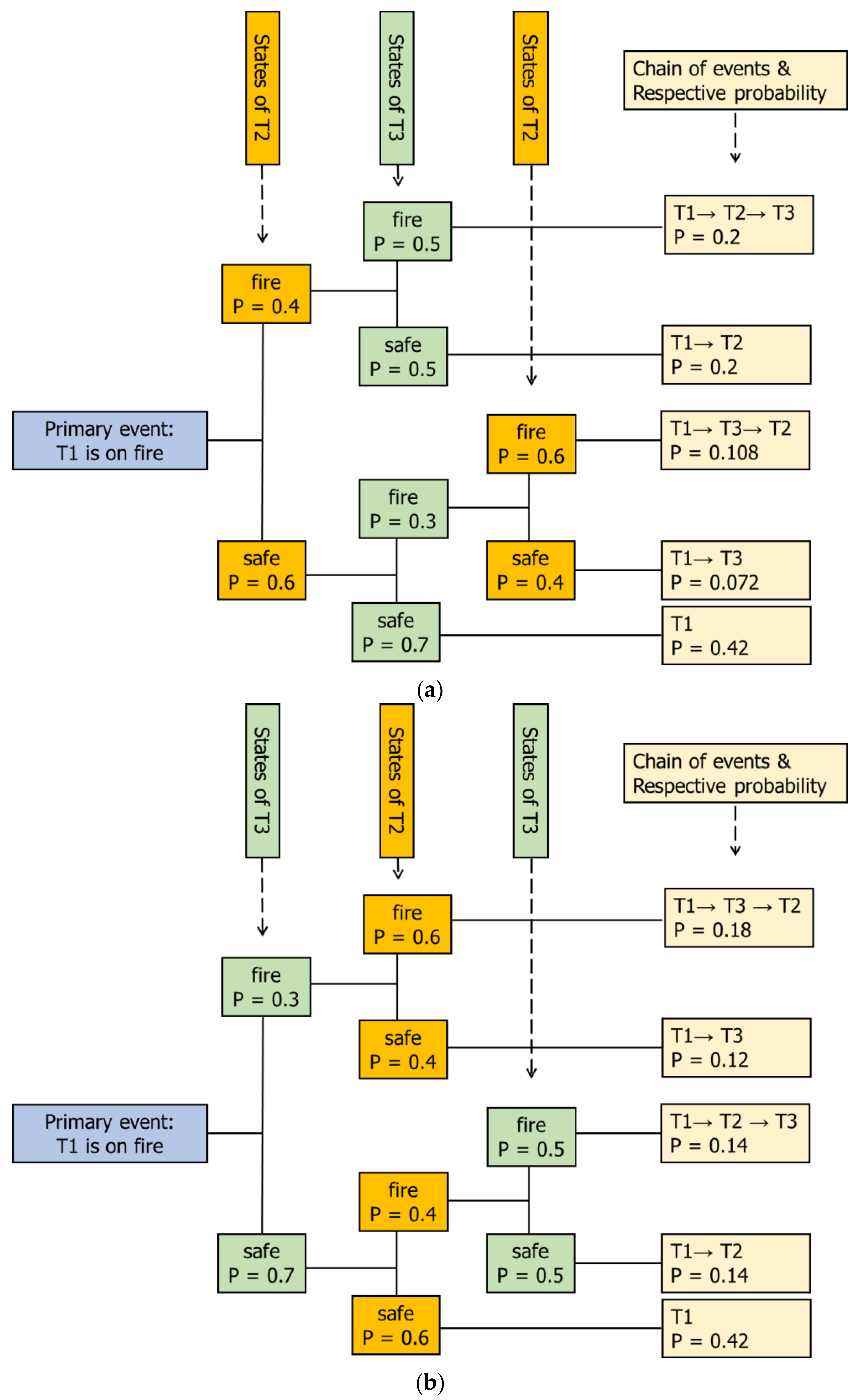
Moreover, for the sake of exemplification, assume that the fire spread probabilities (generally known as the escalation probabilities) have been calculated as P(T2 = fire|T1 = fire, T3 = safe) = 0.4, P(T2 = fire|T1 = fire, T3 = fire) = 0.6, P(T3 = fire|T1= fire, T2= safe) = 0.3, and P(T3 = fire|T1 = fire, T2 = fire) = 0.5.
Considering the event tree as one of the most popular QRA techniques for determining the outcome of an undesired event (initiating event), an analyst may develop the event tree in Figure 2a to identify both the sequence of fires given a fire at T1 and their probabilities while another analyst may choose to employ the event tree in Figure 2b.
As can be seen from Figure 2, even though both event trees are logically equivalent, they result in different probabilities for the same sequence of events. For instance, the probability of P(T1 = fire, T2 = fire) is calculated as 0.2 using the event tree in Figure 2a but 0.14 using the event tree in Figure 2b.
Further, in Figure 2a, the most probable sequence of events is identified as T1→T2→T3 with a respective probability of 0.2 while in Figure 2b the most probable sequence of events is T1→T3→T2 with a corresponding probability of 0.18. As pointed out by Khakzad et al. [25], the reason for obtaining different probabilities for the same sequence of events by using conventional QRA techniques (here, event tree analysis) lies in the limitation of such techniques in considering all possible domino scenarios all at once. As a result, a modeler has no choice but to impose their subjective judgement as for which event tree to choose and thus overlooks the other possibilities.
Among the techniques used to model and assess the risk of domino effects [1,2], BN has been demonstrated to be able to more accurately identify the most probable sequence of events given accurate escalation probabilities. Advances in BN approaches and development of a variety of software for modeling and analysing BNs have enabled a more accurate dynamic risk assessment of domino effects [10,18]. Modeling features of BN and its derivatives facilitate the consideration of spatial-temporal dependencies of domino effects and make it possible to identify the most probable sequence of events in more accurately.
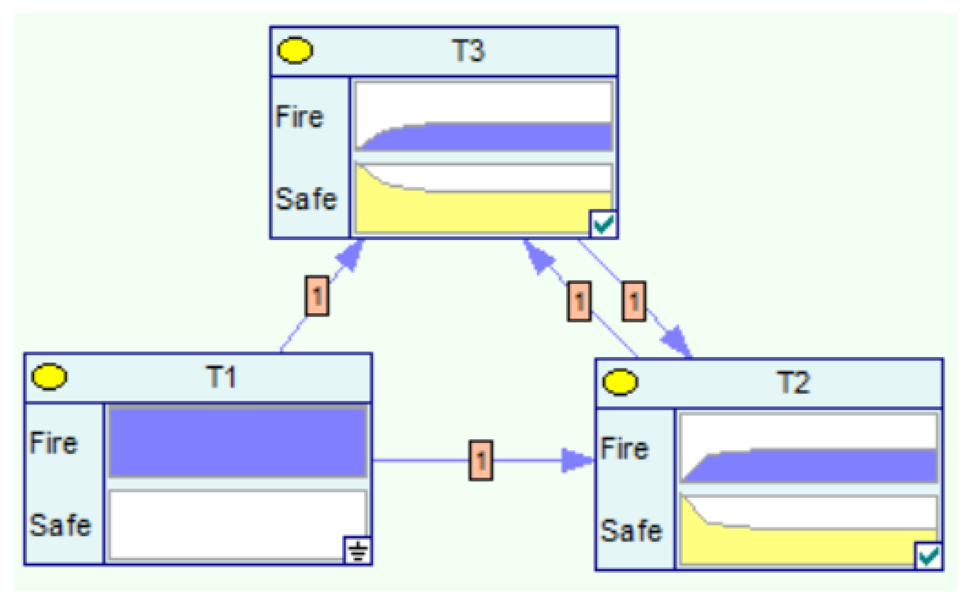
Figure 3 depicts a dynamic Bayesian network (DBN) model for modeling the previous domino effect scenarios given the fire at T1. The DBN allows the modeler to recognize the uncertainty embedded in the spread of fire between T2 and T3 via temporal arcs. Applications of BN and DBN to domino effect modeling are discussed in more detail in the next sections.
Given the same escalation probabilities and taking advantage of probability updating aspect of the BNs, the probabilities of different scenarios are calculated as:
- P(T1→T2→T3) = 0.14, which is equal the one obtained in Figure 2b.
- P(T1→T3→T2) = 0.0108, which is equal to the one obtained in Figure 2a.
- P(T1→T2) = 0.28 and P(T1→T3) = 0.18, neither of which being equal to those obtained in Figure 2a,b.
- Unlike the event tree, which is incapable of calculating the probability of simultaneous fire spread from T1 to both T2 and T3, the developed DBN calculates such probability as P(T1→T2 & T3) = 0.12.
Basics of the BN, DBN, and influence diagram are revisited in Section 2; applications of BN and DBN to domino effect modeling are illustrated in Section 3. In Section 4, applications of DBN and influence diagram to domino effect mitigation and risk management, including optimal firefighting, are demonstrated. While Section 3 and Section 4 are mainly based on the literature, Section 5 is relatively novel, discussing an innovative application of noisy OR to modeling complex domino effects. The work is concluded in Section 6.
2. Bayesian Networks
2.1. Conventional Bayesian Network
A BN [26] is a probabilistic model BN = (G, θ) for reasoning under uncertainty, where G is the model structure in the form of a directed acyclic graph, and θ is the model parameters in the form of conditional probabilities required to quantify the model. G presents the conditional dependencies among the nodes (random variables) of the graph by means of directed arcs—drawn from the parent nodes to the child nodes—while the conditional probabilities assigned to the child nodes in the form of conditional probability tables (CPTs) determine the type of the dependencies. The nodes with no parents (known as root nodes) are assigned marginal probabilities.
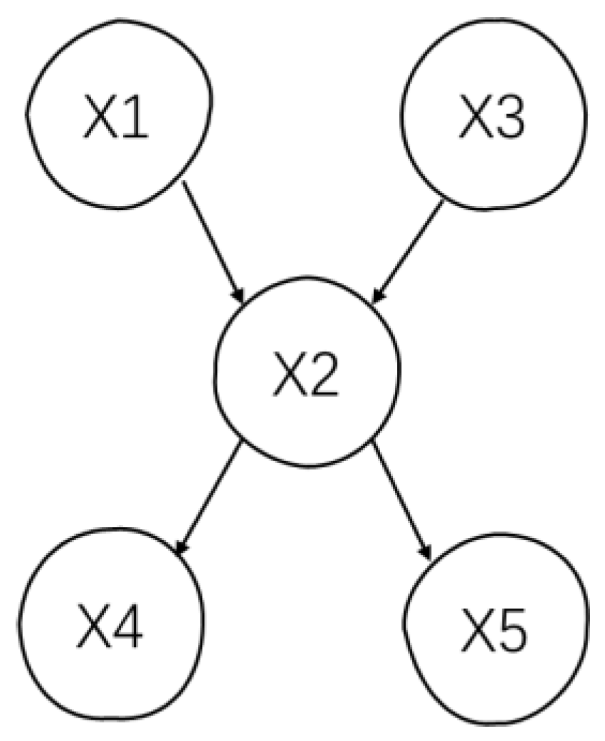
BN takes advantage of the d-separation rule to simplify the joint probability distribution of its nodes. Figure 4 shows a typical BN, and considering the d-separation rule:
- in a serial connection as the one that consists of X1, X2, and X5, if the state of X2 is known, X1 and X5 become conditionally independent: P(X5|X1, X2) = P(X5|X2);
- in a divergent connection as the one that consists of X2, X4, and X5, if the state of X2 is known, X4 and X5 become conditionally independent: P(X5|X2, X4) = P(X5|X2);
- in a convergent connection as the one that consists of X1, X2, and X3, if the state of X2 is unknown, X1 and X3 become independent: P(X1|X3) = P(X1).
The d-separation rule can be manifested as the Markovian property: Given its parents, a node becomes conditionally independent of all its non-descendants. For instance, P(X5|X1, X2) = P(X5|X2) and P(X5|X2, X4) = P(X5|X2). Satisfying the Markovian property, the joint probability distribution of the variables in a BN can be factorized as the product of the nodes’ conditional probabilities given their immediate parents. Considering the BN in Figure 2: P(X1, X2, X3, X4, X5) = P(X1) P(X3) P(X2|X1, X3) P(X4|X2) P(X5|X2). In general:
where , and is the parent set of the node , and n is the number of the BN nodes.
The main application of BN is in probability updating. BN takes advantage of Bayes’ theorem to update the probability of variables given new information—evidence E—to yield the updated (or posterior) probability:
2.2. Dynamic Bayesian Network
A BN can be extended to a DBN to model the dynamic and temporal interdependencies embedded in the sequence of events. To form a DBN, a BN is usually replicated in time slices over a specific time period if the transitional probabilities between the sequential slices could be considered stationary (constant).
Figure 5 displays a two-slice DBN. The arc from X3 to its copy X3′ implies the temporal changes of X3 (e.g., aging of X3) while the arc from X5 to X2′ may either indicate a reciprocal cause-effect relationship (X2→X5→X2) or represent the uncertainty about the sequence of failures (X2→X5 or X5→X2?). It is worth noting that neither of these modeling features can be accommodated in a conventional (static) BN. The joint probability distribution of the nodes of a DBN can be presented in the same way as in a conventional BN.
2.3. Influence Diagram
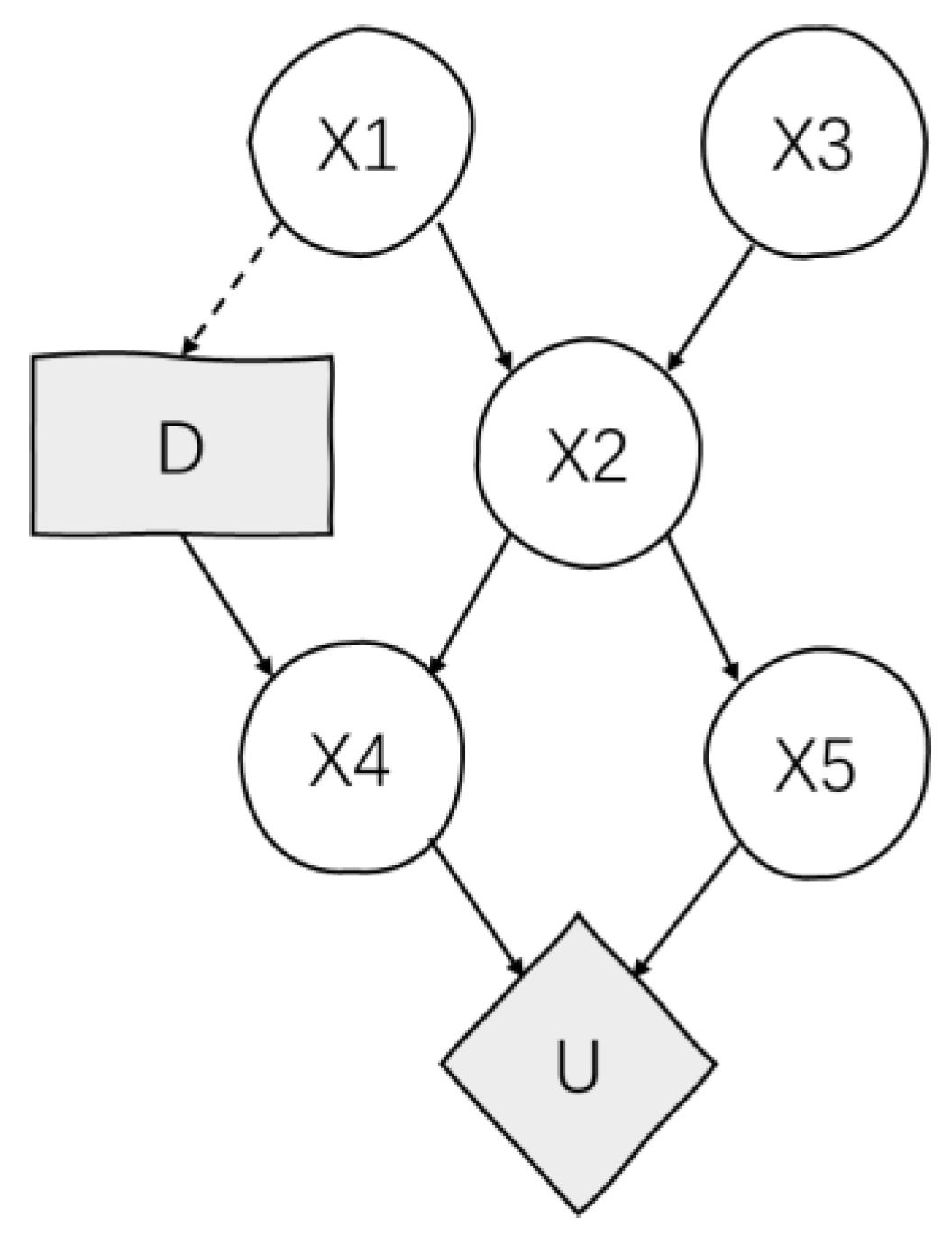
A BN can be extended to an influence diagram (Figure 6) using two additional types of nodes, i.e., decision and utility nodes [26]. In order to visually distinguish decision and utility nodes from chance nodes, decision nodes are conventionally displayed as a rectangle while utility nodes are presented as a diamond.
Each decision node consists of a finite set of decision alternatives as its states. A decision node should be assigned as the parent of all those chance nodes whose probability distributions depend on at least one of the decision alternatives (e.g., X4 in Figure 6). Likewise, the decision node should be the child of all those chance nodes the states of which have to be known to the decision maker before making that specific decision (e.g., X1 in Figure 6).
A utility node expresses the preferences of the decision maker as to the outcomes of the decision alternatives. Each utility node is attributed to a utility table in which the numbers are not probabilities (unlike CPT) but rather utility values (positive or negative) determined by the decision maker for each configuration of parent nodes, either decision nodes or chance nodes [26]. As a result, the decision alternative with the maximum expected utility can be selected as the optimal decision. Utility values are usually determined according to the preferences of the decisionmaker, expressing how much the decision maker prefers one outcome over another outcome.
3. Domino Effect Modeling
3.1. Application of Bayesian Network
Khakzad et al. (2013) developed a methodology based on BN for modeling domino effects in process plants, presenting the process units as the nodes of the BN and the possibility of accident propagation among the adjacent nodes as the directed arcs of the BN. In their approach, the conditional probabilities assigned to the nodes were determined using dose-response relationships (probit functions) developed for estimating the damage probability of process units exposed to heat flux (in the event of fire) and shock wave (in the event of explosions) [8].
Given a primary fire or explosion at a process vessel, among two exposed vessels the one with the highest (conditional) escalation probability is chosen as the secondary unit which would be entailed in the chain of accidents. Considering the possible synergistic effects between the primary and secondary vessels, the sequence and the probabilities of tertiary and higher order vessels getting involved in the chain of accidents can be identified in the same way.
It should be noted that since the explosions are sudden and short-lived, the possibility of having multiple coincident explosions is very low, and thus the principle of synergy rarely applies to the explosions. In the event of fires, however, the possibility of concurrent fires is much higher: industrial fires such as tank fires, pool fires, and jet fires usually take a longer time to burnout (depending on the available fuel) or be suppressed, and thus it is more likely that the heat fluxes of contemporary fires can be superimposed, resulting in a synergistic effect.
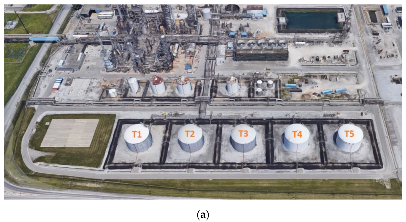
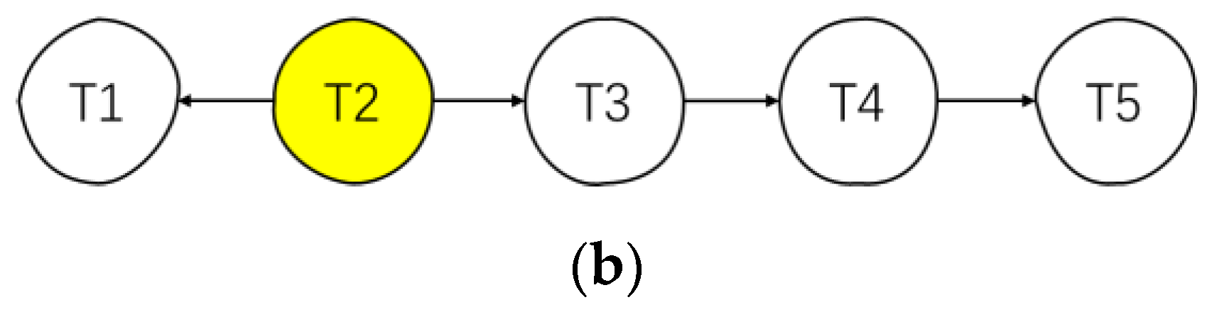
The application of the BN-based methodology [10] to modeling domino effect can be demonstrated using a tank terminal consisting of five fuel storage tanks as shown in Figure 7a. Considering a primary tank fire at T2, the fire spread between the tanks can be modeled as the BN in Figure 7b.
The arc from T2 to T3 denotes the possibility of fire spread from T2 to T3 with a certain probability, depending on the intensity of the heat flux T3 receives from T2 and the type of T3 (atmospheric or pressurized) and its dimension. Likewise, if T3 catches fire, the fire may spread to T4, indicated by the arc from T3 to T4.
As previously mentioned, the conditional escalation probabilities of type P(T3 = fire|T2 = fire) can be determined using dose-response relationships (probit functions). In this example, for illustrative purposes, let’s assume that the escalation probabilities can be estimated as , where Qij is the intensity of the heat flux tank Tj receives from fire at tank Ti. The numerator denotes the heat radiation threshold of 15 kW/m2 required to cause damage to atmospheric storage tanks [8]. Assuming that the intensity of heat radiation each of the storage tanks may receive from an adjacent tank fire is 40 kW/m2, the CPT of node T3 given a tank fire at T2 can be presented as Table 1, where . Since the tanks are identical and exposed to identical heat radiation intensity (40 kW/m2), the same CPT can be assigned to all of them. (Except T2, which is the root node and needs a marginal probability table rather than a CPT).
Implementing the BN in the Bayesian network modeling software, GeNIe [27], the probability of fire spread to each storage tank can be calculated as depicted in Figure 8. Rank ordering the units based on their marginal probabilities, T1 and T3 can be identified as the secondary units: P(T1 = fire) = P(T3 = fire) = 0.63; T4 as the tertiary unit: P(T4 = fire) = 0.39, and T5 as the quaternary unit: P(T5 = fire) = 0.24. These probabilities make sense as the probability of a lower-order event (e.g., a secondary fire at T3) should be higher than the probability of a higher-order event (e.g., a tertiary fire at T4).
The application of BN to domino effect modeling does not capture the uncertainty arising from different possible accident propagation paths. In the tank terminal in Figure 7, for instance, if there were two simultaneous primary fires at T2 and T5, two different BNs (Figure 9) could be developed to model the fire spread.
Having two BNs with the only difference in the direction of the arc between T3 and T4 makes it almost impossible to choose between these two BNs particularly that each BN results in different probabilities for the units. As for developing the CPTs, consider the BN in Figure 9a as an example: the CPTs of T1 and T3 are the same as Table 1, but the CPT of T4 is the same as Table 2 to account for the synergistic effect of T3 and T5 on T4. As such, P(T4 = fire|T3 = safe, T5 = fire) = while P(T4 = fire|T3 = fire, T5 = fire) = .
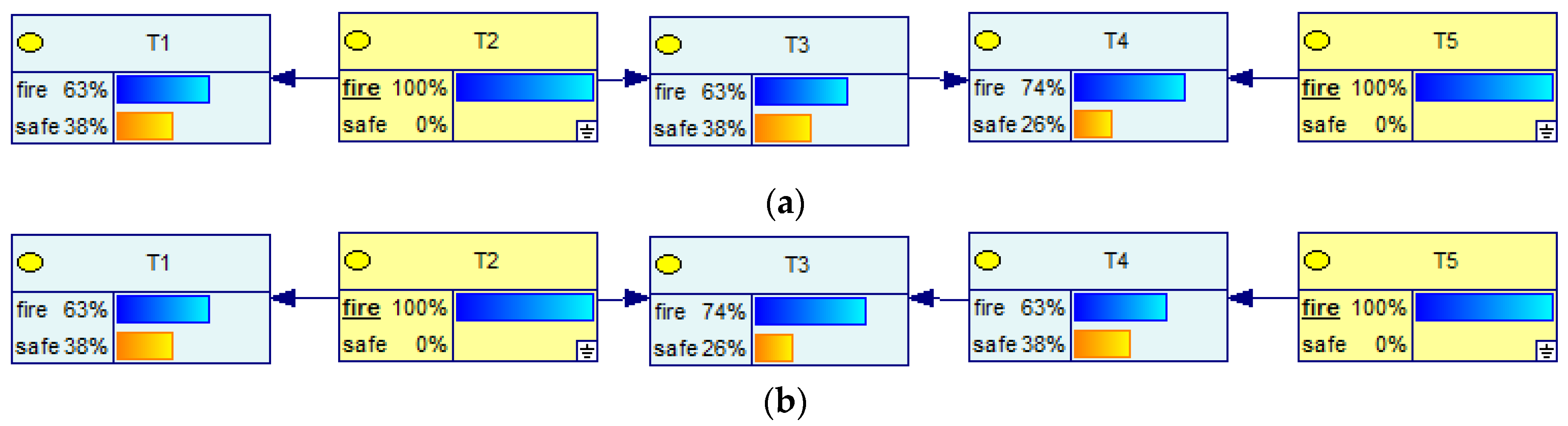
Using the BN in Figure 9a, the probabilities can be calculated as displayed in Figure 10a. Rank ordering the units based on their marginal probabilities, T4 is identified as the secondary unit with a probability of P(T4 = fire) = 0.74, and both T1 and T3 as the tertiary units with an identical probability of P(T1 = fire) = P(T3 = fire) = 0.63. This result, however, does not comply with the structure of the BN: Since T4 would catch fire as a secondary unit before T3 catches fire as a tertiary unit, the direction of the arc—which also implies the sequence of the fires—should be from T4 to T3 not the opposite, unlike what is shown in Figure 10a.
This may make the modeler wonder if the BN in Figure 9b should have been chosen to model the right order of fires during the domino effect. Using the BN of Figure 9b, the probabilities can be calculated as in Figure 10b; as can be seen, again the probabilities of the sequential fires do not comply with the sequence of the fires: structurally and considering the direction of the arcs, T4 seems to catch fire before T3 (note the arc from T4 to T3), however the fire probability at T3 (74%) is higher than that of T4 (63%), which means, T3 has caught fire before T4!
3.2. Application of Dynamic Bayesian Network
As demonstrated in the previous section, the application of conventional BN to domino effect modeling may result (not always) in counterintuitive results (e.g., the probability of a secondary event is less than that of a tertiary event!) This is mainly because the conventional BN is not capable of considering all possible mutual interactions among the involved units, and thus the propagation paths are imposed by the modeler rather than being identified by the model. In other words, the modeler decides about the direction of arcs instead of letting the model identify the most probable path and subsequently align the direction of arcs [25].
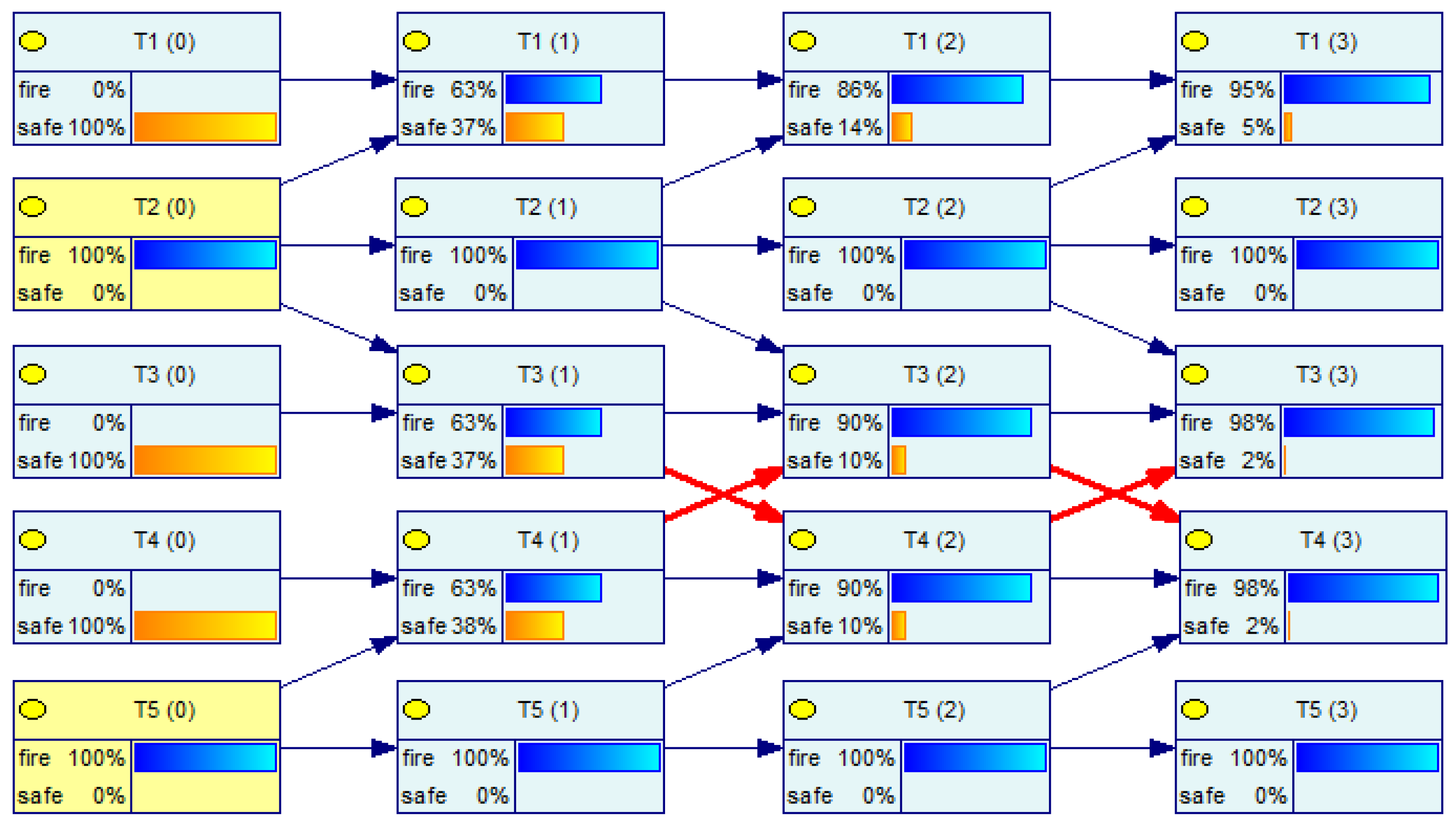
Khakzad [18] modified the BN methodology previously developed by Khakzad et al. [10] by using a DBN, where the most likely sequence of events can be identified by the model by considering all the possible interactions among the units. In this regard, the uncertainty on the temporal sequence of T3 and T4 in Figure 9 can be modeled as the DBN in Figure 11. The arcs in color red denote the uncertainty as to whether the fire would spread from T3 to T4 or the opposite.
In Figure 11, the states of T2 and T5 in the first time slice have been instantiated to “fire” as P(T2(0) = fire) = P(T5(0) = fire) = 100%, whereas the states of T1, T3, and T4 have been instantiated to “safe” as P(T1(0) = safe) = P(T3(0) = safe) = P(T4(0) = safe) =100% as the initial evidence (observation) required to quantify the DBN. The CPTs of the nodes of the DBN in Figure 11 are similar to Table 1 and Table 2. For the sake of clarity, the CPT of T3 in the 2nd time slice, i.e., T3(2), following the tank fires at T2 and T5 in the 0th time slice (the beginning of the modeling) is presented in Table 3.
As can be seen from Figure 11, the DBN results in identical probabilities of fire spread to T3 and T4 at sequential time steps due to the symmetrical position of T3 and T4 to the primary units T2 and T5. In the 1st time step, the probability of fire spread to T1, T3 and T4 is the same as 0.63 mainly because the DBN has not yet be given sufficient time to take into account all the possible fire interactions [25]. Given enough time, the probabilities of fire spread to T3 and T4 are seen to be identical and slightly higher than that of T1. As such, either all the three tanks (T1, T3, T4) may catch fire as the secondary units in the 1st time step with a probability of 0.63 (this is the worst-case scenario) or T3 and T4 may catch fire before T1 in the 2nd time step.
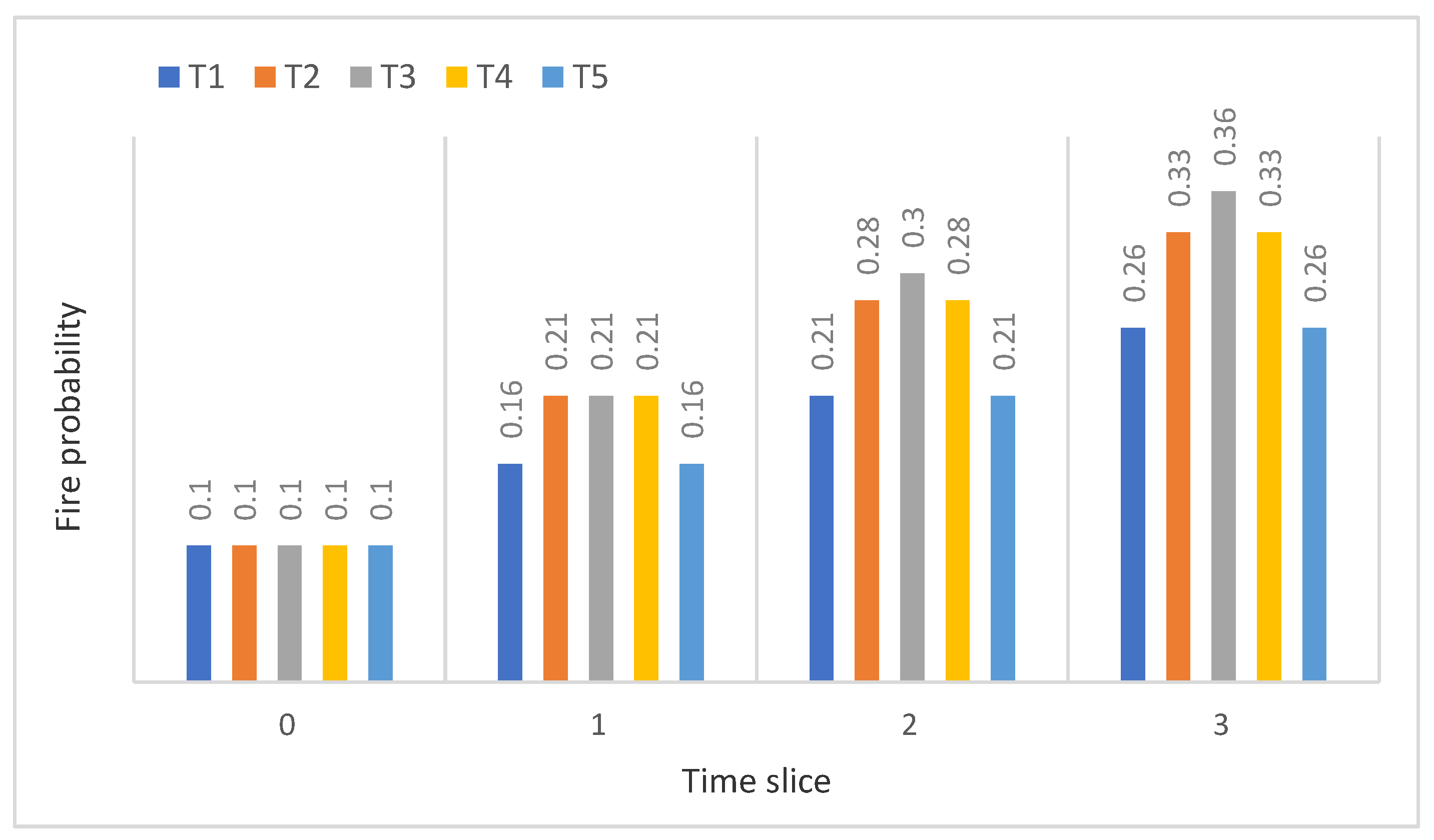
The developed DBN can also be used to identify the most critical units contributing to the domino scenarios [24,28]. For this purpose, given an equal chance of primary fire for all the units at the 0th time slice (0.1, for illustrative purposes) and considering the mutual interactions among all the units, the (marginal) probability of fire spread to each unit can be calculated as shown in Figure 12.
As can be seen, T3 has the highest probability of catching fire as time goes by and thus can be identified as the most critical (vulnerable) unit in the terminal. Khakzad and Reniers [28] demonstrated that the isolation of most vulnerable units from the chain of fires, for instance, via fireproofing or by keeping them empty, would dramatically disrupt the domino effect and thus reduce the vulnerability of the facility more than would the isolation of any other tanks.
4. Domino Effect Mitigating
4.1. Modeling of Add-On Fire Protection Systems
Fire protection systems such as sprinkler systems, water deluge systems, and fireproofing are commonly known as add-on safety systems and are used in the chemical and process plants to prevent, control, and mitigate domino effects. Sprinkler systems are typically installed on atmospheric tanks to mitigate the radiating heat in case of burning tanks or to reduce the absorbed heat in case of exposed tanks. Water deluge systems have a similar function but are typically installed on pressurized vessels. A fireproof coating is usually applied to pressurized vessels and is aimed at reducing the absorbed heat for a limited amount of time.
In this section we demonstrate how the impact of add-on fire systems on domino effects can be modeled via DBN. Interested readers may refer to [29] for a more detailed modeling of different types of fire protection systems in BN and DBN. Consider a generic add-on safety system (B) which has been installed on T2 to suppress fire at T2, which would also mitigate the heat T1 and T3 would receive from T2. To model the safety system in the DBN, assume that:
- B has three states: Active, No-active (idle), and Failed.
- By default, B is in the no-active state but can be activated with a certain probability (1–PFD) if T2 catches fire. PFD is B’s probability of failure on demand.
- When activated, B may still fail with a constant failure rate λ (this assumption can easily be relaxed if need be), resulting in an exponential failure probability of , where t is the time lapse since the activation of B.
- Once activated and put into operation, B will mitigate the emitting heat from T2 with a factor ( < 1) as so that the possibility of damage to adjacent tanks (T1 and T3) and hence the probability of fire spread to them can be reduced. Qm is the mitigated heat emitted from T2 given that B is active; Qo is the original heat emitted from T2 before the activation of B, and α is the mitigating factor.
- B, if successfully activated and keep operating, may extinguish the fire with a certain probability .
- B cannot be repaired. Thus, once it fails it remains in the failed state throughout the modeling.
- As soon as T2 is extinguished, B is back to the idle state (no_active). This assumption has been made for simplification. In reality, B keeps working for a while to ensure T2 does not reignite.
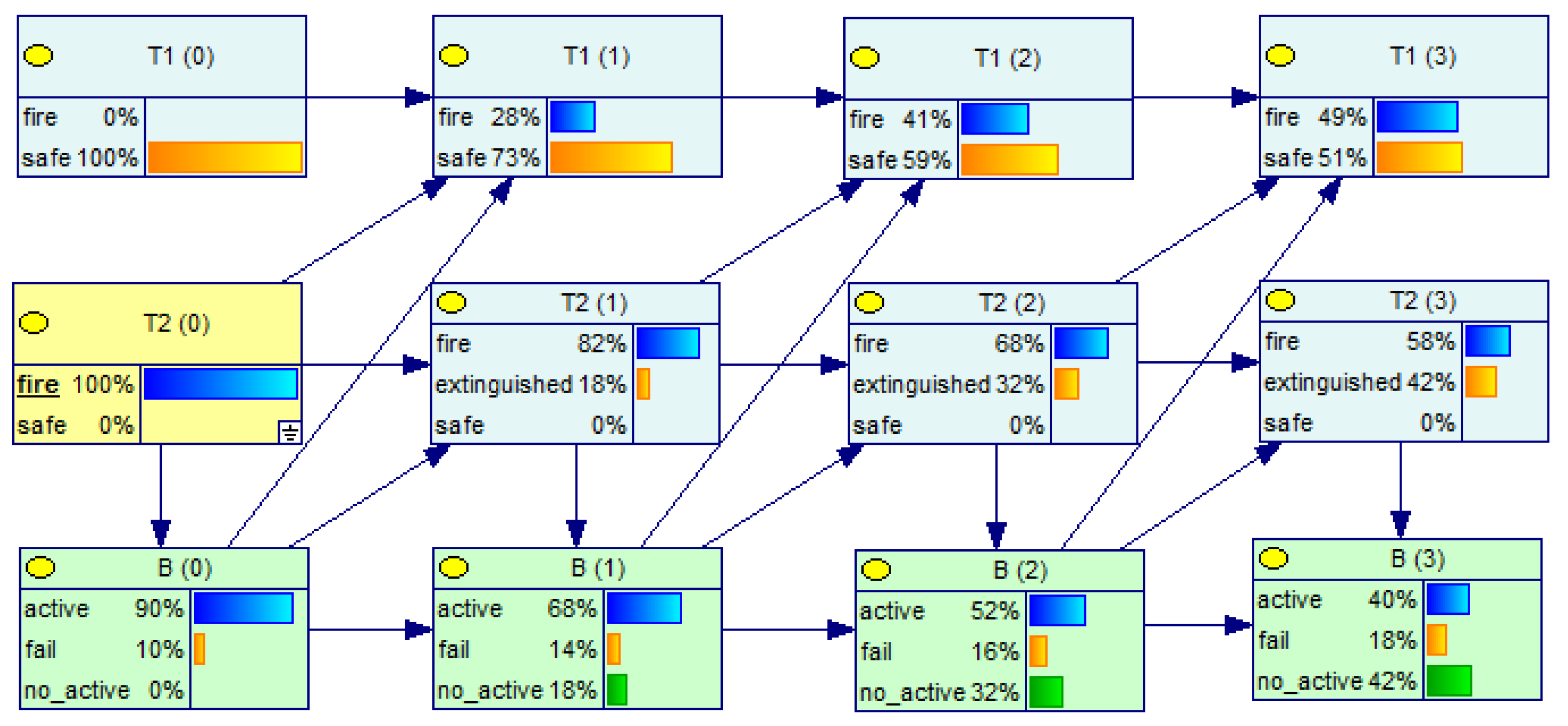
Considering the exemplary values of PFD = 0.1, PB = 0.05 (λ = 0.1 hr−1, and t = 30 min), α = 0.5, and Pe = 0.2 for B, the fire spread from T2 to T1 can be modeled using the DBN in Figure 13. The CPTs of the barrier at the 0th and 1st time slices are presented in Table 4 and Table 5, respectively.
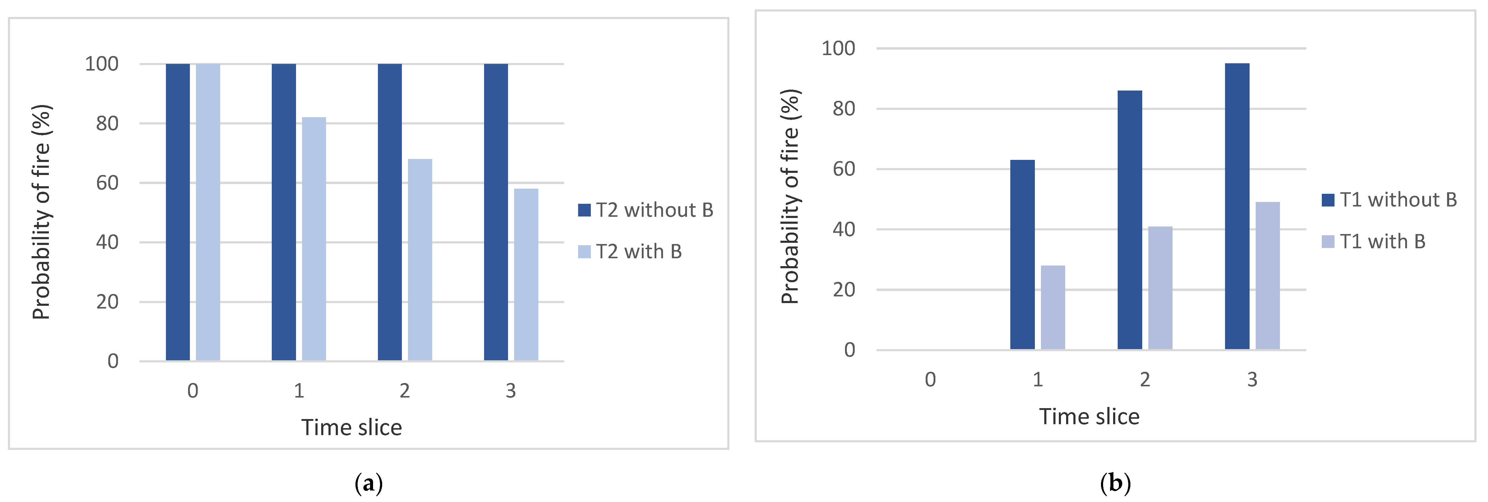
For the sake of clarity, the CPTs of T1 and T2 at the 1st time slice have been presented in Table 6 and Table 7. In Table 6, P(T1(1) = fire|T1(0) = safe, T2(0) = fire, B(0) = active) = . To see the impact of B on the fire escalation of T2 and T1, their fire probabilities with and without the impact of B have been compared in Figure 14a,b.
4.2. Modeling of Firefighting
Firefighting plays a key role in preventing or delaying fire spread. The role of firefighting becomes even more important considering the possibility of damage or malfunction of add-on safety systems [29] or insufficient firefighting resources [19,30,31]. The effectiveness of firefighting strongly depends on the number, skills and the level of preparedness of firefighting crews as well as the amount and the type of firefighting equipment.
When the amount of firefighting crews and required equipment are sufficient, a firefighting team can deal with all the burning and exposed vessels to stop or reduce the possibility of fire spread and thus prevent further damage. However, the main challenge arises when the number of vessels in danger—both on fire and exposed to fire—exceeds the available firefighting resources (staff, equipment, etc.). Accordingly, setting optimal firefighting strategies to identify which burning vessels to suppress and which exposed vessels to protect can become challenging due to limited resources [31].
Industrial firefighting strategies can be (i) passive, in which the burning vessels are left to burn out without any intervention (usually in case of jet fires), (ii) defensive, in which the exposed vessels are cooled mainly using water, or (iii) offensive, where attempts are made to extinguish burning vessels using water-based foam.
During an offensive strategy, the emitted heat from a burning vessel that is under extinguishment will gradually decrease until the fire is completely suppressed. Ignoring the temporal variation, the mitigated heat radiation (Qm) can be taken as a fraction (0 < α < 1) of the original heat radiation Qm = α × Qo; the lower the α, the higher the efficiency of extinguishment. Likewise, during a defensive strategy, the reduced amount of heat received by an exposed vessel (Qc) can be taken as a fraction (0 < β < 1) of the original heat Qc = β × Qo; the lower β, the higher the efficiency of cooling. As a result, in a mixed strategy, the reduced amount of heat a protected vessel would receive from a burning vessel under suppression would be Qmc = α × β × Qo.
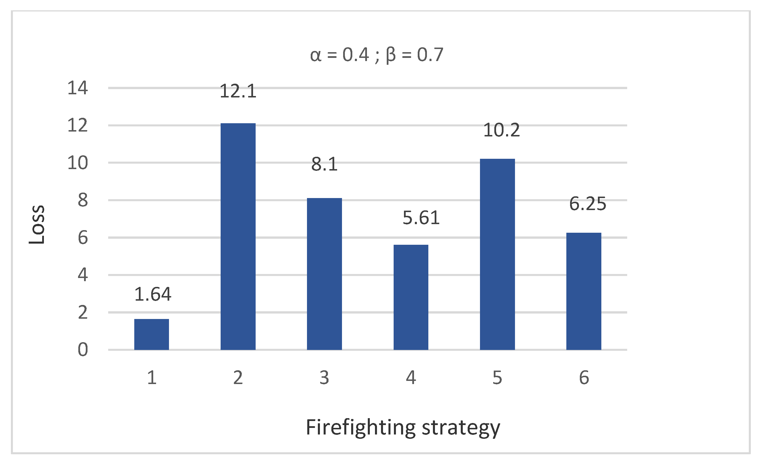
Consider the same tank terminal in Figure 7a. Assume a case where a fire at T2 has already spread to T3 by the time the firefighters deploy their resources. Further, assume that available resources do not allow the firefighters to work on more than two tanks at a time. As only two tanks can be included in the firefighting endeavor, six strategies can be considered for firefighting as listed in Table 8. Moreover, to account for the possible inefficiency of firefighting, consider these firefighting efficiencies: α = 0.4 and β = 0.7.
Figure 15 displays the escalation of fire from T2 and T3 to the other tanks. For the sake of clarity, the CPT of node T4 given the fire at T3 is presented in Table 9.
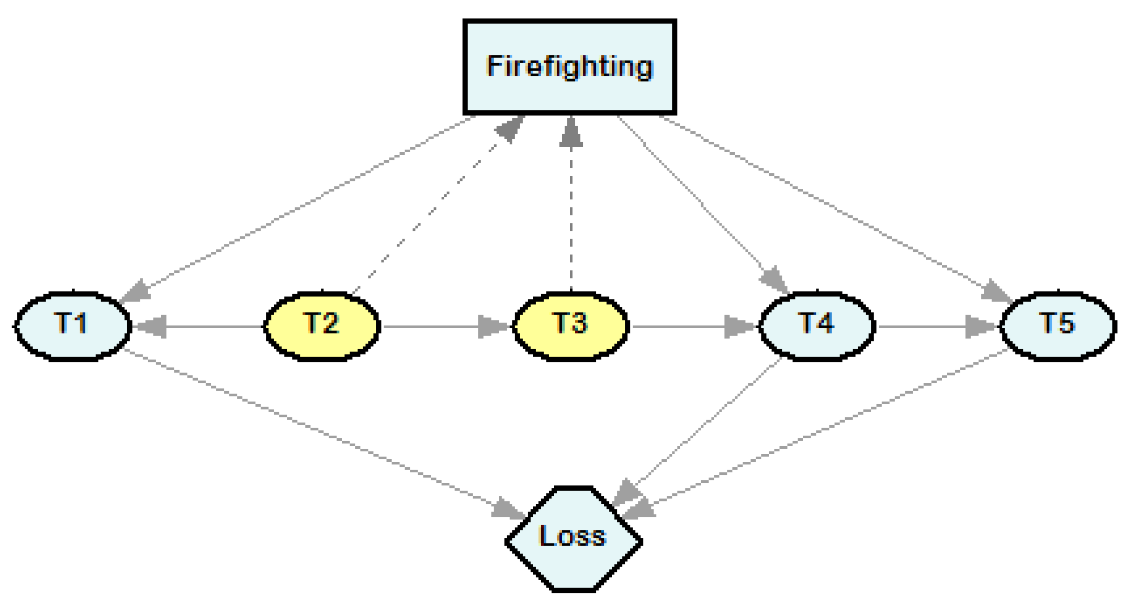
As can be noted, the BN has been converted into an influence diagram by adding the decision node “Firefighting” and the utility node “Loss”. The node “Firefighting” incorporates the six firefighting strategies listed in Table 8 as the decision alternatives. The effect of the decision policies on the nodes can be reflected by making modifications to the nodes’ conditional probability tables (escalation probabilities). The procedure for modifying the conditional probability table of T4 under the influence of the decision node is presented in Table 10.
- (a)
- P(T4 = Fire|T3 = Fire, d1) = 1 − = 0.06.
- (b)
- Since the amount of Q34 is below the threshold (0.4 × 0.7 × 40 = 11.2 < 15 kW/m2), it would not cause damage and fire spread to T4.
In Figure 15, the utility node “Loss” has been connected to the still safe storage tanks, T1, T4, and T5, so that only further damage caused from the spread of fire from T2 and T3 can be taken into account in the decision making. Since the storage tanks are identical, any damaged storage tank is assumed to be associated with a loss value of –10. For example, U(T1 = Fire, T4 = Fire, T5 = Safe) = −20.
Modeling the influence diagram in GeNIe [27], the expected loss of firefighting strategies can be calculated and used to make a comparison among the firefighting strategies in Figure 16. The strategy attributed with the lowest loss, i.e., d1 in this case, can be selected as the optimal strategy. A more complicated application of dynamic influence diagrams to optimal firefighting can be found in [31].
5. Application of Noisy-OR
As previously demonstrated, DBN can be used as a robust technique in modeling domino effects by identifying the most contributing events and the sequential entailment of the events in the chain of accidents. Compared to ordinary BN, DBN provides the modeler with much more flexibility in modeling interdependencies both spatially and temporally, which is not feasible in an ordinary BN. However, some modeling issues still need to be addressed to enhance the performance of DBN and increase the accuracy or the results.
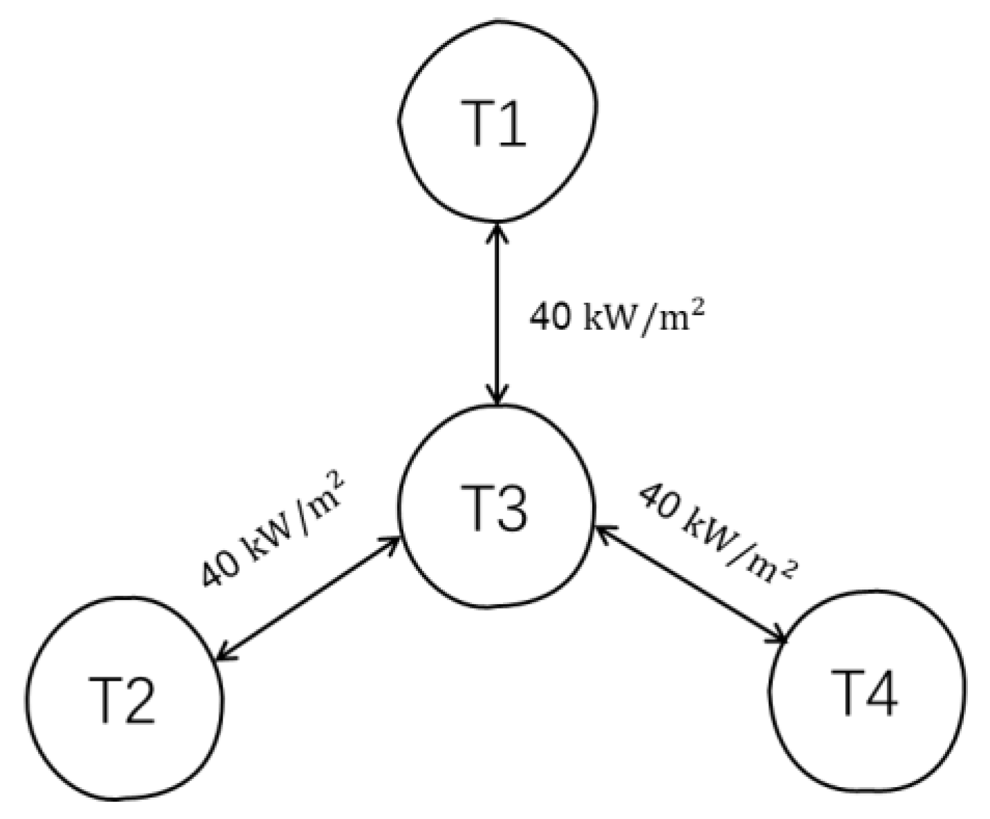
The notion of synergistic effects during fire domino effects refers to the confluence of concurrent fires on a target unit. This, in turn, may lead to an exponential growth of the conditional probability table of the target unit as the number of concurrent fires in the vicinity of the unit increases. For example, consider a different but still simple arrangement of tanks T1–T4 in Figure 17, where a burning tank can radiate the heat flux 40 kW/m2 to the other tanks.
Considering the mutual interactions and possible synergistic effects and only two states for each node (safe, fire), 15 probabilities should be identified for the CPT of T3. Such probabilities are in the form of, for instance:
P(T3t+1 = fire | T3t = safe, T1t = fire, T2t = safe, T4t = fire) = .
The size of the CPTs can readily grow out of hand and become intractable for a more complex arrangement of the units. To alleviate the exponential growth of the CPTs due to synergistic effects of simultaneous fires, the Noisy-OR technique can be employed. (Noisy-OR was first proposed by Khakzad et al. [10] to account for the leak probability—probability of a unit catching fire during a domino accident due to other unknow reasons than fire spread from adjacent units, for instance, self-ignition of the unit.)
The Noisy-OR takes advantage of causal independency to reduce the number of required conditional probabilities from 2m–1 to m, where m is the number of binary parents of the child node. The Noisy-OR model is only applicable to binary variables as a special case of a more general Noisy-MAX model, which is applicable to multi-state variables.
The Noisy-OR model requires all the causes (parents) of an effect (child node) be present in the BN, where each cause (Ci) is capable of causing the effect (e) with a respective probability as:
Pi = P(e = true|C1 = false, C2 = false, …, Ci = true, Ci+1 = false, …Cn = false)
As such, the probability of the effect given any combination of its active causes can be calculated as:
where C is the active causes. Thus, when all the causes of the effect are false:
Since , using the Noisy-OR model, the foregoing conditional probability of T3t+1 can be calculated as:
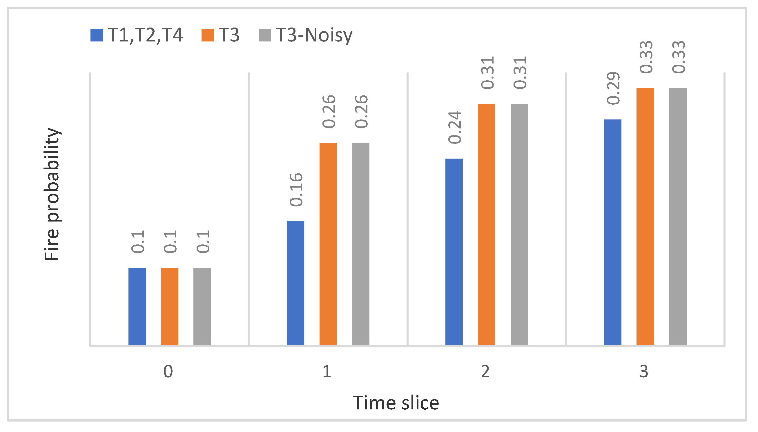
P(T3t+1 = fire|T3t = safe, T1t = fire, T2t = safe, T4t = fire) = 1 − (1 − 0.625) (1 − 0.625) = 0.859. As can be seen, the conditional probability of T3t+1 which is calculated using the Noisy-OR model, i.e., 0.859, is in good agreement with the one calculated without the Noisy-OR model, i.e., 0.813.
Figure 18 displays the fire spread probabilities of the tanks, in which the probabilities calculated for T3 with and without the Noisy-OR model are identical.
6. Conclusions
In the present study, we exemplified some applications of the BN, DBN, and influence diagram in the modeling of fire domino effects. It was illustrated that even for a very simple case study, the application of conventional QRA techniques such as event tree analysis can result in misleading and inconsistent probabilities and chains of accidents.
On the other hand, the BN and particularly DBN were shown to result in more consistent results by considering complicated spatial-temporal interdependencies and uncertainties, which cannot be considered in the event tree analysis. Despite offering a great deal of flexibility and robustness in modeling and reasoning, the application of DBN to highly dynamic and complex domino scenarios may nevertheless result in intractable conditional probability tables (CPTs), which can be too large to handle. This issue, however, was demonstrated to be greatly alleviated via the application of the Noisy-OR model. Nevertheless, the application of Noisy-OR to developing the CPTs still needs further verification via more complex and larger case studies before it can be reliably used for this purpose. Another research topic which is worth investigating in the future studies is the application of dynamic influence diagrams—as an extension of DBN—to dynamic decision making and risk management of domino effects. The models discussed in the present study can readily be extended to modeling and risk management of other types of cascading effects in a variety of systems or infrastructures provided that they can be modeled as networks.
Funding
This research received no external funding.
Institutional Review Board Statement
Not applicable.
Informed Consent Statement
Not applicable.
Conflicts of Interest
The author declares no conflict of interest.
References
- Swuste, P.; van Nunen, K.; Reniers, G.; Khakzad, N. Domino effects in chemical factories and clusters: An historical perspective and discussion. Process Saf. Environ. Prot. 2019, 124, 18–30. [Google Scholar] [CrossRef]
- Chen, C.; Reniers, G.; Khakzad, N. A thorough classification and discussion of approaches for modeling and managing domino effects in the process industries. Saf. Sci. 2020, 125, 104618. [Google Scholar] [CrossRef]
- Bagster, D.F.; Pitblado, R.M. The estimation of domino incident frequencies—An approach. Process Saf. Environ. Prot. 1991, 69, 195–199. [Google Scholar]
- Khan, F.; Abbasi, S. Simulation of accidents in a chemical industry using the software package MAXCRED. Indian J. Chem. Technol. 1996, 3, 338–344. [Google Scholar]
- Khan, F.I.; Abbasi, S. Models for domino effect analysis in chemical process industries. Process Saf. Prog. 1998, 17, 107–123. [Google Scholar] [CrossRef]
- Khan, F.I.; Abbasi, S. An assessment of the likelihood of occurrence, and the damage potential of domino effect (chain of accidents) in a typical cluster of industries. J. Loss Prev. Process Ind. 2001, 14, 283–306. [Google Scholar] [CrossRef]
- Cozzani, V.; Salzano, E. Threshold values for domino effects caused by blast wave interaction with process equipment. J. Loss Prev. Process Ind. 2004, 17, 437–447. [Google Scholar] [CrossRef]
- Cozzani, V.; Gubinelli, G.; Antonioni, G.; Spadoni, G.; Zanelli, S. The assessment of risk caused by domino effect in quantitative area risk analysis. J. Hazard. Mater. 2005, 127, 14–30. [Google Scholar] [CrossRef]
- Van der Voort, M.M.; Klein, A.J.J.; de Maaijer, M.; van den Berg, A.C.; van Deursen, J.R.; Versloot, N.H.A. A quantitative risk assessment tool for the external safety of industrial plants with a dust explosion hazard. J. Loss Prev. Process Ind. 2007, 20, 375–386. [Google Scholar] [CrossRef]
- Khakzad, N.; Khan, F.; Amyotte, P.; Cozzani, V. Domino effect analysis using Bayesian networks. Risk Anal. 2013, 33, 292–306. [Google Scholar] [CrossRef]
- Landucci, G.; Molag, M.; Cozzani, V. Modeling the performance of coated LPG tanks engulfed in fires. J. Hazard. Mater. 2009, 172, 447–456. [Google Scholar] [CrossRef]
- Dadashzadeh, M.; Khan, F.; Hawboldt, K.; Amyotte, P. An integrated approach for fire and explosion consequence modelling. Fire Saf. J. 2013, 61, 324–337. [Google Scholar] [CrossRef]
- Dadashzadeh, M.; Ahmad, A.; Khan, F. Dispersion modelling and analysis of hydrogen fuel gas released in an enclosed area: A CFD-based approach. Fuel 2016, 184, 192–201. [Google Scholar] [CrossRef]
- Baalisampang, T.; Abbassi, R.; Garaniya, V.; Khan, F.; Dadashzadeh, M. Fire impact assessment in FLNG processing facilities using Computational Fluid Dynamics (CFD). Fire Saf. J. 2017, 92, 42–52. [Google Scholar] [CrossRef]
- Rum, A.; Landucci, G.; Galletti, C. Coupling of integral methods and CFD for modeling complex industrial accidents. J. Loss Prev. Process Ind. 2018, 53, 115–128. [Google Scholar] [CrossRef]
- Alileche, N.; Olivier, D.; Estel, L.; Cozzani, V. Analysis of domino effect in the process industry using the event tree method. Saf. Sci. 2017, 97, 10–19. [Google Scholar] [CrossRef]
- Chen, C.; Khakzad, N.; Reniers, G. Dynamic vulnerability assessment of process plants with respect to vapor cloud explosions. Reliab. Eng. Syst. Saf. 2020, 200, 106934. [Google Scholar] [CrossRef]
- Khakzad, N. Application of dynamic Bayesian network to risk analysis of domino effects in chemical infrastructures. Reliab. Eng. Syst. Saf. 2015, 138, 263–272. [Google Scholar] [CrossRef]
- Zhou, J.; Reniers, G.; Khakzad, N. Application of event sequence diagram to evaluate emergency response actions during fire-induced domino effects. Reliab. Eng. Syst. Saf. 2016, 150, 202–209. [Google Scholar] [CrossRef]
- Zhou, J.; Reniers, G. Petri-net based cascading effect analysis of vapor cloud explosions. J. Loss Prev. Process Ind. 2017, 48, 118–125. [Google Scholar] [CrossRef]
- Kamil, M.Z.; Taleb-Berrouane, M.; Khan, F.; Ahmed, S. Dynamic domino effect risk assessment using Petri-nets. Process Saf. Environ. Prot. 2019, 124, 308–316. [Google Scholar] [CrossRef]
- Reniers, G.; Dullaert, W. DomPrevPlanning©: User-friendly software for planning domino effects prevention. Saf. Sci. 2007, 45, 1060–1081. [Google Scholar] [CrossRef]
- Khakzad, N.; Reniers, G. Using graph theory to analyze the vulnerability of process plants in the context of cascading effects. Reliab. Eng. Syst. Saf. 2015, 143, 63–73. [Google Scholar] [CrossRef] [Green Version]
- Khakzad, N.; Reniers, G.; Abbassi, R.; Khan, F. Vulnerability analysis of process plants subject to domino effects. Reliab. Eng. Syst. Saf. 2016, 154, 127–136. [Google Scholar] [CrossRef]
- Khakzad, N.; Amyotte, P.; Cozzani, V.; Reniers, G.; Pasman, H. How to address model uncertainty in the escalation of domino effects? J. Loss Prev. Process Ind. 2018, 54, 49–56. [Google Scholar] [CrossRef]
- Pearl, J. Probabilistic Reasoning in Intelligent Systems; Morgan Kaufmann: San Francisco, CA, USA, 1988. [Google Scholar]
- GeNIe 2.3. Decision Systems Laboratory, University of Pittsburg. December 2018. Available online: https://download.bayesfusion.com/files.html?category=Academia (accessed on 22 December 2018).
- Khakzad, N.; Reniers, G. Low-capacity utilization of process plants: A cost-robust approach to tackle man-made domino effects. Reliab. Eng. Syst. Saf. 2019, 191, 106114. [Google Scholar] [CrossRef]
- Khakzad, N.; Landucci, G.; Reniers, G. Application of dynamic Bayesian network to performance assessment of fire protection systems during domino effects. Reliab. Eng. Syst. Saf. 2017, 167, 232–247. [Google Scholar] [CrossRef] [Green Version]
- Khakzad, N. Which fire to extinguish first? A risk-informed approach to emergency response in oil terminals. Risk Anal. 2018, 38, 1444–1454. [Google Scholar] [CrossRef] [Green Version]
- Khakzad, N. Optimal firefighting to prevent domino effects: Methodologies based on dynamic influence diagram and mathematical programming. Reliab. Eng. Syst. Saf. 2021, 212, 107577. [Google Scholar] [CrossRef]
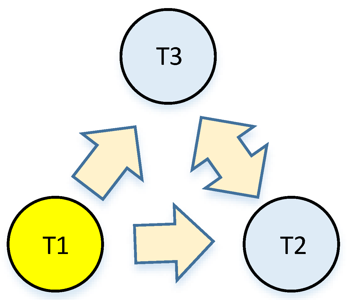
Figure 1.
A tank farm consisting of three fuel storage tanks. Given a primary tank fire at T1, the possibility of fire spread to the other tanks has been denoted with arrows. The double-head arrow represents the uncertainty regarding the direction of fire spread between T2 and T3.
Figure 1.
A tank farm consisting of three fuel storage tanks. Given a primary tank fire at T1, the possibility of fire spread to the other tanks has been denoted with arrows. The double-head arrow represents the uncertainty regarding the direction of fire spread between T2 and T3.

Figure 2.
Event tree analysis for identifying the sequence of events given a tank fire at T1. The sequence of the fires and the respective probabilities are given at the end of the event tree branches. The event trees are logically equivalent but structurally different: (a) T2 is considered as the first top event on the event tree. (b) T3 is considered as the first top event on the event tree.

Figure 3.
Application of DBN to domino effect modeling which may be initiated by a fire at T1. The uncertainty regarding the direction of fire spread between T2 and T3 is represented using two temporal arcs between T2 and T3, depending on which first catches fire.
Figure 3.
Application of DBN to domino effect modeling which may be initiated by a fire at T1. The uncertainty regarding the direction of fire spread between T2 and T3 is represented using two temporal arcs between T2 and T3, depending on which first catches fire.

Figure 4.
A generic Bayesian network.

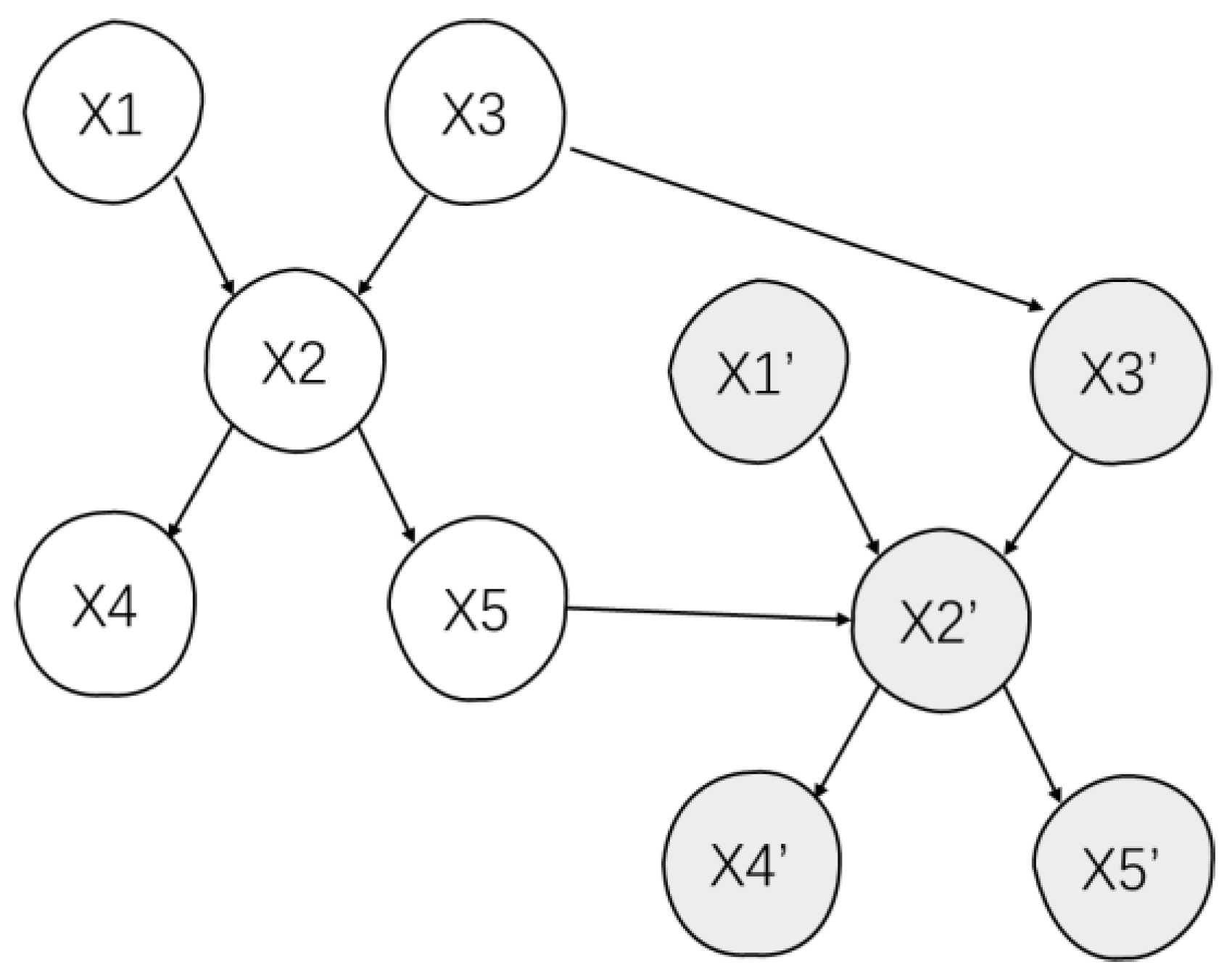
Figure 5.
A generic DBN. The arc from X3 to its copy in the second time slice X3′ shows the temporal evolution of X3. The arcs from X2 to X5 to X2′ may either represent the mutual impact of X2 and X5 or model the uncertainty as to whether X2 is the parent of X5 or the opposite.
Figure 5.
A generic DBN. The arc from X3 to its copy in the second time slice X3′ shows the temporal evolution of X3. The arcs from X2 to X5 to X2′ may either represent the mutual impact of X2 and X5 or model the uncertainty as to whether X2 is the parent of X5 or the opposite.

Figure 6.
An influence diagram by adding decision node D and a utility node U to the Bayesian network.
Figure 6.
An influence diagram by adding decision node D and a utility node U to the Bayesian network.

Figure 7.
(a) A process plant consisting of five atmospheric storage tanks of gasoline, T1-T5. (b) Likely spread of fire given a primary fire at T2.
Figure 7.
(a) A process plant consisting of five atmospheric storage tanks of gasoline, T1-T5. (b) Likely spread of fire given a primary fire at T2.


Figure 8.
Modeling of fire domino using BN given a primary tank fire at T2.

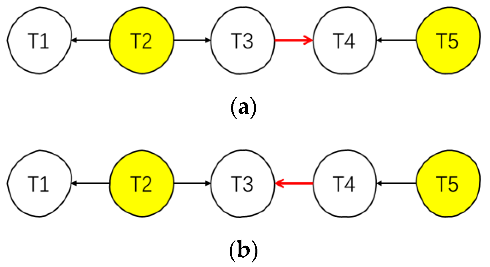
Figure 9.
(a) BN for modeling domino scenario starting from T2 and T5 given that T3 catches fire before T4. (b) BN for modeling the same fire domino given that T4 catches fire before T3.
Figure 9.
(a) BN for modeling domino scenario starting from T2 and T5 given that T3 catches fire before T4. (b) BN for modeling the same fire domino given that T4 catches fire before T3.

Figure 10.
Counterintuitive results obtained for the application of conventional BN to domino effect modeling. (a) T3 has a lower probability, but the arc from T3 to T4 implies that T3 has caught fire before T4, and thus its probability should have been higher than that of T4. (b) T4 has a lower probability, but the arc from T4 to T3 implies that T4 has caught fire before T3.

Figure 11.
Modeling fire domino as a DBN given tank fires at T2 and T5. The arcs in color red denote the uncertainty as to whether the fire would spread from T3 to T4 or the opposite.
Figure 11.
Modeling fire domino as a DBN given tank fires at T2 and T5. The arcs in color red denote the uncertainty as to whether the fire would spread from T3 to T4 or the opposite.

Figure 12.
Temporal changes of fire spread probabilities given equal chances of fire (p = 0.1) for all the tanks at t = 0. Tank T3 has the highest probability of catching fire as time goes by and thus can be identified as the most critical (vulnerable) unit.
Figure 12.
Temporal changes of fire spread probabilities given equal chances of fire (p = 0.1) for all the tanks at t = 0. Tank T3 has the highest probability of catching fire as time goes by and thus can be identified as the most critical (vulnerable) unit.

Figure 13.
Modeling the impact of safety system (B) on the fire spread from T2 to T1.

Figure 14.
(a) Evolution of the temporal probabilities of (a) T2 and (b) T1, with and without the impact of the safety system.
Figure 14.
(a) Evolution of the temporal probabilities of (a) T2 and (b) T1, with and without the impact of the safety system.

Figure 15.
Influence diagram to identify optimal firefighting strategies given fires at T2 and T3. (These two nodes have been highlighted with color yellow). The dotted arcs from T2 and T3 to the decision node “firefighting” imply that the optimal firefighting strategy is identified given the observation of fire at T2 and T3.

Figure 16.
Comparison of firefighting strategies based on their expected loss.

Figure 17.
A hypothetical tank arrangement. Heat fluxes (kW/m2) radiated from and absorbed by the adjacent tanks in case of tank fires are denoted on the arrows.
Figure 17.
A hypothetical tank arrangement. Heat fluxes (kW/m2) radiated from and absorbed by the adjacent tanks in case of tank fires are denoted on the arrows.

Figure 18.
Fire spread probabilities with and without Noisy-OR model given equal probabilities of fire (0.1) at the 0th time slice. The probabilities of T1, T2, and T4 grow equally due to their symmetrical position to one another.
Figure 18.
Fire spread probabilities with and without Noisy-OR model given equal probabilities of fire (0.1) at the 0th time slice. The probabilities of T1, T2, and T4 grow equally due to their symmetrical position to one another.


Table 1.
CPT of T3 given a tank fire at T2.
| P(T3|T2) | ||
|---|---|---|
| T2 | fire | safe |
| fire | 0.63 | 0.37 |
| safe | 0.00 | 1.00 |
Table 2.
CPT of T4 in Figure 9a given the primary tank fires at T2 and T5.
Table 2.
CPT of T4 in Figure 9a given the primary tank fires at T2 and T5.
| P(T4|T3,T5) | |||
|---|---|---|---|
| T5 | T3 | fire | safe |
| fire | fire | 0.81 | 0.19 |
| fire | safe | 0.63 | 0.37 |
| safe | fire | 0.63 | 0.37 |
| safe | safe | 0.00 | 1.00 |
Table 3.
Conditional probability table of T3(2) given tank fires at T2(0) and T5(0).
| P(T3(2)|T2(1),T3(1),T4(1)) | ||||
|---|---|---|---|---|
| T3(1) | T2(1) | T4(1) | Fire | Safe |
| fire | fire | fire | 1.00 | 0.00 |
| fire | fire | safe | 1.00 | 0.00 |
| fire | safe | fire | 1.00 | 0.00 |
| fire | safe | safe | 1.00 | 0.00 |
| safe | fire | fire | 0.81 | 0.19 |
| safe | fire | safe | 0.63 | 0.37 |
| safe | safe | fire | 0.63 | 0.37 |
| safe | safe | safe | 0.00 | 1.00 |
Table 4.
Conditional probability table of the safety system at the 0th time slice, B(0).
| P(B(0)|T2(0)) | |||
|---|---|---|---|
| T2(0) | Active | Fail | No_Active |
| fire | 1 − PFD = 0.9 | PFD = 0.1 | 0 |
| safe | 0.0 | 0.0 | 1.0 |
Table 5.
Conditional probability table of the safety system at the 1st time slice, B(1).
| P(B(1)|B(0),T2(1)) | ||||
|---|---|---|---|---|
| B(0) | T2(1) | Active | Failed | No_Active |
| active | fire | 1 − Pt = 0.95 | Pt = 0.05 | 0 |
| active | extinguished | 0 | 0 | 1 |
| active | safe | 0 | 0 | 1 |
| failed | fire | 0 | 1 | 0 |
| failed | extinguished | 0 | 1 | 0 |
| failed | safe | 0 | 1 | 0 |
| no_active | fire | 1 − PFD = 0.9 | PFD = 0.1 | 0 |
| no_active | extinguished | 0 | 0 | 1 |
| no_active | safe | 0 | 0 | 1 |
Table 6.
Conditional probability table of T1 at the 1st time slice, T1(1).
| P(T1(1)|T1(0), T2(0), B(0)) | ||||
|---|---|---|---|---|
| T1(0) | T2(0) | B(0) | Fire | Safe |
| fire | fire | active | 1 | 0 |
| fire | fire | failed | 1 | 0 |
| fire | fire | no_active | 1 | 0 |
| fire | safe | active | 1 | 0 |
| fire | safe | failed | 1 | 0 |
| fire | safe | no_active | 1 | 0 |
| safe | fire | active | 0.25 | 0.75 |
| safe | fire | failed | 0.63 | 0.37 |
| safe | fire | no_active | 0.63 | 0.37 |
| safe | safe | active | 0 | 1 |
| safe | safe | failed | 0 | 1 |
| safe | safe | no_active | 0 | 1 |
Table 7.
Conditional probability table of T2 at the 1st time slice, T2(1).
| P(T2(1)|T2(0), B(0)) | ||||
|---|---|---|---|---|
| T2(0) | B(0) | Fire | Extinguished | Safe |
| fire | active | 1 − Pe = 0.8 | Pe = 0.2 | 0 |
| fire | failed | 1 | 0 | 0 |
| fire | no_active | 1 | 0 | 0 |
| safe | active | 0 | 0 | 1 |
| safe | failed | 0 | 0 | 1 |
| safe | no_active | 0 | 0 | 1 |
Table 8.
Firefighting strategies given fires at T2 and T3.
| Firefighting Strategy | Description |
|---|---|
| d1 | Extinguish both T2 and T3 |
| d2 | Cool both T1 and T4 |
| d3 | Extinguish T2 and cool T4 |
| d4 | Extinguish T3 and cool T1 |
| d5 | Extinguish T2 and cool T1 |
| d6 | Extinguish T3 and cool T4 |
Table 9.
Conditional probability table of T4 in Figure 15.
Table 9.
Conditional probability table of T4 in Figure 15.
| T3 | P(T4|T3) | |
|---|---|---|
| Fire | Safe | |
| Fire | 0.63 | 0.37 |
| Safe | 0 | 1 |
Table 10.
Conditional probabilities of T4 given fire at T3 and different firefighting strategies for α = 0.4 and β = 0.7 and. Q34 is the heat flux T4 receives from T3.
Table 10.
Conditional probabilities of T4 given fire at T3 and different firefighting strategies for α = 0.4 and β = 0.7 and. Q34 is the heat flux T4 receives from T3.
| Strategy | Firefighting Policy | Q34 (kW/m2) | P(T4|T3 = Fire, di) | |
|---|---|---|---|---|
| Fire | Safe | |||
| d1 | Extinguish both T2 and T3 | 0.4 × 40 | 0.06 a | 0.94 |
| d2 | Cool both T1 and T4 | 0.7 × 40 | 0.46 | 0.54 |
| d3 | Extinguish T2 and cool T4 | 0.7 × 40 | 0.46 | 0.54 |
| d4 | Extinguish T3 and cool T1 | 0.4 × 40 | 0.06 | 0.94 |
| d5 | Extinguish T2 and cool T1 | 40 | 0.63 | 0.37 |
| d6 | Extinguish T3 and cool T4 | 0.4 × 0.7 × 40 | 0.00 b | 1.00 |
Publisher’s Note: MDPI stays neutral with regard to jurisdictional claims in published maps and institutional affiliations. |
© 2021 by the author. Licensee MDPI, Basel, Switzerland. This article is an open access article distributed under the terms and conditions of the Creative Commons Attribution (CC BY) license (https://creativecommons.org/licenses/by/4.0/).
Share and Cite
MDPI and ACS Style
Khakzad, N. A Tutorial on Fire Domino Effect Modeling Using Bayesian Networks. Modelling 2021, 2, 240-258. https://0-doi-org.brum.beds.ac.uk/10.3390/modelling2020013
AMA Style
Khakzad N. A Tutorial on Fire Domino Effect Modeling Using Bayesian Networks. Modelling. 2021; 2(2):240-258. https://0-doi-org.brum.beds.ac.uk/10.3390/modelling2020013
Chicago/Turabian StyleKhakzad, Nima. 2021. "A Tutorial on Fire Domino Effect Modeling Using Bayesian Networks" Modelling 2, no. 2: 240-258. https://0-doi-org.brum.beds.ac.uk/10.3390/modelling2020013