Article

A Machine Learning-Aided Network Contention-Aware Link Lifetime- and Delay-Based Hybrid Routing Framework for Software-Defined Vehicular Networks

by
Patikiri Arachchige Don Shehan Nilmantha Wijesekara
* and
Subodha Gunawardena
Department of Electrical and Information Engineering, Faculty of Engineering, University of Ruhuna, Galle 80000, Sri Lanka
*
Author to whom correspondence should be addressed.
Submission received: 8 June 2023 / Revised: 23 June 2023 / Accepted: 5 July 2023 / Published: 18 July 2023

Abstract

:
The functionality of Vehicular Ad Hoc Networks (VANETs) is improved by the Software-Defined Vehicular Network (SDVN) paradigm. Routing is challenging in vehicular networks due to the dynamic network topology resulting from the high mobility of nodes. Existing approaches for routing in SDVN do not exploit both link lifetimes and link delays in finding routes, nor do they exploit the heterogeneity that exists in links in the vehicular network. Furthermore, most of the existing approaches compute parameters at the controller entirely using heuristic approaches, which are computationally inefficient and can increase the latency of SDVN as the network size grows. In this paper, we propose a novel hybrid algorithm for routing in SDVNs with two modes: the highest stable least delay mode and the highest stable shortest path mode, in which the mode is selected by estimating the network contention. We distinctly identify two communication channels in the vehicular network as wired and wireless, where network link entropy is formulated accordingly and is used in combination with pending transmissions to estimate collision probability and average network contention. We use the prospect of machine learning to predict the wireless link lifetimes and one-hop channel delays, which yield very low Root Mean Square Errors (RMSEs), depicting their very high accuracy, and the wireless link lifetime prediction using deep learning yields a much lower average computational time compared to an optimization-based approach. The proposed novel algorithm selects only stable links by comparing them with a link lifetime threshold whose optimum value is decided experimentally. We propose this routing framework to be compatible with the OpenFlow protocol, where we modify the flow table architecture to incorporate a route valid time and send a packet_in message to the controller when the route’s lifetime expires, requesting new flow rules. We further propose a flow table update algorithm to map computed routes to flow table entries, where we propose to incorporate an adaptive approach for route finding and flow rule updating upon reception of a packet_in message in order to minimize the computational burden at the controller and minimize communication overhead associated with control plane communication. This research contributes a novel hybrid routing framework for the existing SDVN paradigm, scrutinizing machine learning to predict the lifetime and delay of heterogeneity links, which can be readily integrated with the OpenFlow protocol for better routing applications, improving the performance of the SDVN. We performed realistic vehicular network simulations using the network simulator 3 by obtaining vehicular mobility traces using the Simulation of Urban Mobility (SUMO) tool, where we collected data sets for training the machine learning models using the simulated environment in order to test models in terms of RMSE and computational complexity. The proposed routing framework was comparatively assessed against existing routing techniques by evaluating the communication cost, latency, channel utilization, and packet delivery ratio. According to the results, the proposed routing framework results in the lowest communication cost, the highest packet delivery ratio, the least latency, and moderate channel utilization, on average, compared to routing in VANET using Ad Hoc On-demand Distance Vector (AODV) and routing in SDVN using Dijkstra; thus, the proposed routing framework improves routing in SDVN. Furthermore, results show that the proposed routing framework is enhanced with increasing routing frequency and network size, as well as at low vehicular speeds.

1. Introduction

Vehicular Ad Hoc Networks (VANETs) are mobile network-based autonomous systems consisting of wirelessly connected mobile vehicles in the transportation sector. However, VANETs have a set of challenges for information dissemination due to frequent topology changes due to high mobility and the presence of isolated nodes. By incorporating the Software-Defined Networking (SDN) concept into VANETs, a new paradigm called Software-Defined Vehicular Network (SDVN) has been developed to overcome the previous challenges. It consists of a logically centralized control plane with a network view that collects data from the vehicular network and makes network decisions based on that view, thereby making vehicular networks more programmable and flexible.
Routing is the process of selecting a path for traffic on a given network. It has been challenging for VANETs, due to their dynamic network topologies resulting from the high mobility of vehicular nodes. There exist numerous routing techniques for routing in VANETs, such as greedy stateless routing using immediate neighbors, distance vector routing on demand, using link states generated by multipoint relays, distance vector routing using periodic broadcasts, etc. In SDVN, routing occurs by modifying flow tables by the centralized controllers based on the metadata collected by the controllers. Heuristic shortest path algorithms, greedy routing algorithms minimizing cost, routing with minimum communication hops, shortest stable path routing, routing with minimum service delay, etc. have been used in SDVN for routing.
However, the problem is that, to the best of our knowledge, a routing algorithm for SDVNs that is based on both link delay and link lifetime has not yet been proposed. In the existing literature, there is only a theoretical approach to estimating an average value for the total delay at each hop, while there is no practical approach for finding the exact total one-hop delay for each communication channel. Furthermore, most existing routing algorithms do not exploit the heterogeneous links existing in vehicular networks, which are wired and wireless. Furthermore, parameter computation at the controller has been conducted entirely by many routing algorithms using heuristic approaches. However, we note that parameter computations, such as link lifetime and link delay calculations using rule-based methods, are computationally complex and can grow with the network size, resulting in the controller not computing routes in a timely manner.
This research focuses on a novel routing algorithm for SDVNs in order to overcome the problems stated above. The proposed routing technique has a hybrid mode with two modes: the highest stable shortest path mode and the highest stable least delay mode, in which the mode is selected based on the network contention. When network contention is low, the highest stable least delay mode is selected, as one-hop channel delay prediction is more accurate under low network contention, and vice versa. For computing network contention, we first distinctly identify the vehicular network as a heterogeneous network consisting of wired (I2I—Infrastructure to Infrastructure) and wireless links (V2V—Vehicle to Vehicle, V2I—Vehicle to Infrastructure, I2V—Infrastructure to Vehicle) and formulate heterogeneous link state entropy and the pending transmission packet distribution factor to predict collision probability. We use a trained Deep Neural Network (DNN) to predict delay at each hop for wired and wireless communication channels when network contention is lower than a specified threshold. According to the best of our knowledge, we were the first to predict the exact one-hop delay at each hop for the two communication channels in SDVNs with the help of machine learning and compute the link delays in the network based on the predictions. For wireless link lifetime prediction, we first formulate it as an optimization problem using first principles and then estimate the wireless link lifetime using another DNN, by using the factors affecting wireless link lifetime prediction such as differential displacement, differential velocity, differential acceleration, remaining distance to maximum wireless transmission distance, etc. We were also the first to use a deep learning approach for wireless link lifetime prediction in SDVNs. Results show that wireless link lifetime prediction using DNN is more computationally efficient than the optimization-based approach while still having high accuracy.
Using the DNNs for link lifetime prediction for wireless links and one-hop delay prediction for both communication channels, adjacency matrices for link lifetime, position, and link delay are computed at the controller to feed into the novel hybrid routing algorithm. The algorithm finds either the highest stable shortest path or the highest stable least delay path from a given source node to each and every other node and returns the parent vector containing the routes. The routing algorithm first chooses its mode using the computed normalized network contention and finds routes to all other nodes as destination nodes iteratively. For a given destination node, if the algorithm is in the most stable shortest path mode, it will first select the communication channel for the edge in the position matrix by inspecting only link lifetimes. However, if the algorithm is in the highest stable least delay mode, it will select the communication channel for the edge in the link delay matrix by inspecting the ratio of link delay and link lifetime for the edge (If the ratio is lower, link delay in that channel will be selected). Furthermore, the algorithm inspects the link lifetime against a threshold value before adding an edge to a route, where the edge will be added to the route if the edge’s link lifetime is greater than the threshold. We decided on the threshold value experimentally. We proposed the routing framework in order to be compatible with the existing OpenFlow protocol, and we proposed to include an additional field “Route valid timestamp” as a statistic in the flow table to track the final timestamp that a matched entry of the flow table is valid for forwarding a packet without contacting the controller for new flow rules. Thus, we effectively prevent packet forwarding on expired paths, which can result in poor packet delivery ratios, by modeling “Route valid timestamp” in flow table architecture. We furthermore proposed an algorithm to update the flow table at the controller using the computed routes from the routing algorithm, where the link lifetime of the weakest link of a computed path is added to the present timestamp in setting the route valid timestamp field, while the Node ID and link types of the source node, the destination node, and the next hop are mapped with the topology database to update the flow table. Not only that, we refrain from the computationally inefficient approach of a proactive approach and utilize an adaptive algorithm to compute routes, update the flow table, and install flow rules, which compare the current timestamp with the route valid timestamp of the flow table at the controller upon reception of a packet_in message, which then computes routes and update the table only if the flow table entry is expired and composes a FlowMod packet and send it to the corresponding switch to update flow rules at the switch. The purpose of the adaptive approach for flow rule updating is to effectively reduce the communication overhead associated with control plane communication and minimize the computational burden at the controller for computing routes. Finally, we present a systematic approach for metadata collection, parameter computation, route finding, flow table updating, and routing scheduling. We further analyze the performance of the proposed routing framework against routing in VANETs using Ad Hoc On-demand Distance Vector (AODV) and routing in SDVN, making use of the Dijkstra shortest path algorithm.
The proposed hybrid routing framework is novel in various aspects. Firstly, we are the first to identify the factors and model exact one-hop channel delay estimation using a machine learning approach for heterogeneous communication channels with the help of network metadata collected by the controller in SDVN. Existing works fail to compute an exact one-hop channel delay, as there exists only a theoretical approach to estimating contention delay in the existing literature. Secondly, the hybrid routing algorithm (Figure 1) is novel in its approach, in that it selects its mode by examining the current network state in the form of normalized network contention, where both modes select the highest stable links. The least distance mode under high network contention selects stable shortest paths, while the least delay mode under low network contention selects stable least delay paths. This hybrid approach has not yet been investigated by any researcher, to the best of our knowledge. Thirdly, the routing framework proposes a novel flow table update algorithm (Figure 2) and an adaptive flow rule computation approach (Figure 3), along with a modified flow table architecture by adding a route-valid timestamp to the OpenFlow flow table structure to update the controller’s flow table. Flow rule computation is adaptive in its approach, which is different from the proactive and reactive approaches found in the existing literature for flow table updating. Finally, a novel systematic approach for the whole routing process, including metadata collection, parameter computations, the flow table update, and unicasting to switches, is presented.
Contributions to the existing literature from this research are listed below:
  • We present a novel hybrid routing algorithm for SDVNs that uses collected metadata from nodes to estimate parameters at the controller to compute routes that yield the least communication cost, the highest packet delivery ratio, the least latency, and moderate channel utilization, on average, compared to routing in VANETs (AODV) and SDVNs (Dijkstra);
  • This research provides insight into the employment of machine learning for accurate and computationally efficient parameter computation at the controller, such as the estimation of link delay and lifetime, satisfying the communication requirements of vehicular networks;
  • This research experimentally investigates the factors under which the proposed hybrid routing framework is enhanced, so that these factors can be effectively used by future researchers to boost the performance of the proposed novel hybrid routing framework;
  • The proposed routing algorithm will be very useful for more efficient dissemination of information in the data plane of future SDVNs than existing approaches.
This routing framework is limited to SDVNs, in which the control plane collects metadata from all vehicle nodes in a logically centralized manner to generate matrices such as link lifetime and link delay, with the help of machine learning and compute parameters such as normalized network contention, in order to compute routes using the proposed algorithm. For instance, the proposed algorithm cannot be applied to a VANET where there is no logically centralized control plane that collects the metadata required to execute the proposed routing algorithm.
The following is an outline of the remainder of the paper. The background on VANETs, SDVNs and their current architectures, routing in SDVN, and the application of machine learning for routing are covered in Section 2’s assessment of the literature. The proposed routing framework is described in depth in Section 3. The metrics for performance evaluation, the setting of the simulation environment, and all the study experiments, with their findings and interpretations, are presented in Section 4. In Section 5, the results are discussed, cross-analyzed, and compared to the body of previous research. The paper concludes and future research is presented in Section 6.

2. Background and Literature Review

2.1. VANET

A VANET depends on the operation of the automobiles themselves and lacks a dedicated communication infrastructure [1]. A VANET is a subclass of a Mobile Ad Hoc Network (MANET), which is an autonomous group of mobile devices working together to offer network features in the absence of a permanent infrastructure. MANETs interact with one another using wireless networks and collaborate with one another in a dispersed fashion [2]. These networks tend to be defined by self-organizing, uncertain, and dynamic linkages between the wireless nodes, as well as variable topologies for the network [3]. The immense mobility of the nodes with changing topologies of the network and the VANETs’ vast number of nodes (vehicles) with tremendous processing capacity are some of the characteristics that clearly separate them from MANETs [4]. Dedicated Short-Range Communication (DSRC), mobility patterns restricted by roadways, and a lack of substantial power limitations are other features of VANETs [5]. A VANET is made up of automobiles that include an On-Board Unit (OBU) that may communicate with other automobiles or Road Side Units (RSUs) [6]. In a VANET, RSUs are immobile nodes for communications that are placed close to the pathways to improve connection [7]. Vehicle-to-Vehicle (V2V) communication refers to communication between motor vehicles, whereas Vehicle-to-Infrastructure (V2I) communication refers to information dissemination between vehicles and other infrastructure, such as RSUs, tariffs, and web access points [8]. V2X, broadly, stands for Vehicle-to-Everything communication. A Vehicular Sensor Network (VSN) is made up of detectors in automobiles and RSUs that can perceive information about traffic or environmental factors, including warmth, motion, stress, shock, etc. These data are analyzed by vehicle applications to produce messages that can be transmitted via the VANET [9]. Applications for VANETs include remote wireless diagnostics, entertainment, driving assistance frameworks, ideal speed recommendation frameworks, and accident alert systems [10]. However, VANETs have their own unique set of difficulties, including high automobile movement, security issues, and routing problems [11].

2.2. SDN

Conventional networking is infrastructure-based, with the control plane dispersed among several routers and other network gear. By logically isolating the fundamental network control mechanism from switches and routers to provide network control centralization, Software Defined Networking (SDN) makes network programming possible [12]. In comparison to conventional hardware-driven networking, SDN provides more network awareness and the capacity to design safe paths by using the controller’s gathering of network status information [13]. SDN has three planes: the infrastructure plane, the control plane, and the application plane. Flexibility and programmability are the main advantages that SDVN adds compared to conventional networks. In SDN, control is conceptually centralized, allowing any number of physical devices to interact via a single protocol. SDN has made it possible to perform new tasks and provide new services, such as traffic optimization, virtualization of networks and automation, cloud-based service coordination, etc. [14]. However, dependability is one of the major drawbacks of SDN, since the SDN controller often acts as one possible point of breakdown [15]. Additionally, SDN encounters difficulties integrating with traditional networks that cannot utilize the OpenFlow protocol, the centralized controller’s being unable to independently control all traffic, the existence of only a handful of protocols for communication between the controller and applications, etc. [16].

2.3. SDVN

A variant of Software-Defined Wireless Network (SDWN), known as a Softwar-Defined Vehicular Network (SDVN), is created by implementing SDN in wireless networks [17]. By implementing SDN in VANETs, a new architecture called SDVN makes vehicular networks configurable and versatile [18]. Numerous benefits are gained as a result of the SDN controller’s network perception, including adaptive node transmission power reservation, improved routing, flexible radio interface placement, etc. [19]. Additionally, SDVN improves networking functions such as routing and balancing of load and makes global optimizations in VANETs because of the collection of network statistics. It also fosters network innovation by allowing innovative protocols for VANETs to be evaluated and executed at a less expense [20]. However, SDVN encounters a number of difficulties, including security gaps [21], difficult network operations such as routing and transmission management because of the extensive mobility of the nodes, and a changeable network topology [22,23].

2.4. SDVN Architectures

Based on the level of control of the SDN controller, there are three SDVN architectures: centralized, distributed, and hybrid [24]. Nodes in the data plane carry out actions in accordance with the traffic rules provided by the SDN controller in a centralized architecture where control is totally conceptually centralized. The control plane connection between the nodes and the centralized controller in this design, however, has resulted in greater latency [25]. Additionally, expansion is limited under this design, and there is a propensity for error when the control plane connection becomes unavailable or interrupted. In a distributed control architecture, control is split among a number of controllers, with the end nodes operating under the direction of local controllers, while the local controllers may be subordinate to a global controller. This design avoids the centralized control architecture’s sole point of breakdown and expansion capability problems. However, because of consistency difficulties, this design takes longer than the centralized architecture to optimize and make choices [26]. To surpass the drawbacks of both distributed control and centralized control systems, a hybrid control architecture has been developed. According to the needs, the centralized controller in this architecture may change the nodes’ level of control from maximal to minimal, acting as a hybrid of centralized and distributed control [27].

2.5. Routing

Routing is a fundamental network function in any network. Due to the multiple-hop network structure that might regularly alter as a result of mobility, routing is difficult in VANETs [28]. Greedy Perimeter Stateless Routing (GPSR), which takes routing decisions based on the immediate neighbor, is one of the routing protocols used in VANETs [29]. Further, Ad Hoc On-demand Distance Vector (AODV) routing, which does not require global periodic routing advertisements, is a distance vector routing protocol in which the routes are obtained on demand [30]. Using the concept of multipoint relays, which are the nodes forwarding broadcast messages during the flooding process, Optimized Link State Routing (OLSR) uses link states generated by the multipoint relays for routing [31]. Using periodic broadcasts to immediate neighbors, routing tables in each of the nodes are updated in the Destination Sequenced Distance Vector (DSDV) routing protocol [32].

2.6. Routing in SDN

In SDN, routing occurs in switches based on flow tables, which are modified by using the logically centralized control plane [33]. The Shortest Path First (SPF) routing algorithm has been used in early SDN [34]. However, this method does not employ network resources in the most effective way. Rule-based (heuristic) algorithms have been used for routing, but these algorithms’ computation complexity has been found to be high, so machine learning can be used to replace such algorithms to reduce the computational cost [35]. A routing protocol for SDN routing in wireless multihop networks with a higher network lifetime was proposed in [36]. The authors in [37] employed a Long Short-Term Memory (LSTM) neural network to predict and learn traffic characteristics in real time and generate forwarding rules to replace heuristic algorithms. Reinforcement Learning (RL) for routing optimization in SDN has shown better Quality of Service (QoS) parameters than the traditional Open Shortest Path First (OSPF) algorithm, according to research conducted in [38]. In these algorithms, the controller serves as the agent, while the network, traffic, and routing serve as the environment, state, and action, respectively. Adaptive routing, which is aware of QoS protocols, is present in multilayer hierarchical SDNs that employ RL and a QoS aware reward function for packet forwarding [39]. Traffic prediction is an important function in routing optimization. Offline traffic load prediction using neural networks has been used to obtain online routing decisions in software-defined mobile metro-core networks [40]. Some use load features (bandwidth utilization ratio, packet loss rate, transmission latency, and transmission hops) to calculate integrated load for different paths using neural networks and choose the one with the least load [41].

2.7. Routing in SDVN

In SDVNs, the traditional routing protocols can fail, as the connection between the SDN controller and the nodes can be lost due to the high mobility of the nodes, so a hierarchical SDVN architecture has been proposed to overcome the routing problem [42]. A network resource scheduling scheme with the objective of minimizing communication costs and a greedy routing algorithm was applied for heterogeneous SDVNs in [43]. An on-demand routing protocol having a two-level design with a Road Side Unit (RSU) as the local controller for selecting vehicles, to forward a packet within a road segment, and a global controller, to select a road segment having higher performance under large networks and high-speed vehicles, was presented in [44]. In [45], a spray-and-pray multiple copy routing system for SDVNs has been provided. It uses graph-based least communication steps to determine the utility of carriers and two-copy cooperative techniques to minimize delivery latency. A routing algorithm to find a globally optimized routing path for vehicles switching between a multihop forwarding model and a carry-and-forward model for SDVN is presented in [46]. Work in [47] not only found the shortest path for packet forwarding in SDVNs, but also considered the effect of link stability in finding optimum paths as vehicular networks are inherently dynamic and connections between vehicles can exist only for a short amount of time. The routing model in [48,49] for SDVN prevents packet crashes, concurrent transmissions, and circular routing by prioritizing the traffic type to minimize service latency and jointly leveraging diverse interfaces to maximize data packet delivery. A routing protocol comprising both centralized and distributed, which is tribrid as it uses multicast, unicast, and store, carry, and forward concepts appropriately to find stable enough shortest routes satisfying QoS parameters in terms of latency, was depicted in [50]. In a hierarchically controlled SDVN, a cognitive routing protocol called CR–SDVN, which senses the spectrum to improve link stability and find a stable path for routing, was investigated in [51]. A clustering algorithm for long-distance routing along with a control communication overhead reduction approach has been proposed along with backup VANET routing in a fog computing-based SDVN environment [52]. Hidden Markov models have been used to predict the location of the destination vehicle in a highway mobility scenario of an SDVN to compute optimal routing paths at the controller [53].

2.8. Machine Learning for Routing in SDVN

Machine Learning (ML) technology has been trending in recent years, and it has been applied for routing optimization [54], trust-based routing optimization [55], etc. in SDVNs. In the method in [56], the routing database is updated using reinforcement learning, and the most stable routing path is determined using multilevel greedy routing with link stability. Recently, distributed Q-learning has been applied to VANETs to update a Q-table maintained in each vehicle node by exchanging messages between the vehicles [57]. Li et al. [58] extended the preceding concept by eliminating the need for routing tables and replacing them with by Q-tables formed by traffic flow in neighboring grids, which divide the VANET into a set of grids and find the optimum sequence of grids from source to destination using Q learning.
We summarize the existing studies for routing in SDVN in Table 1. However, as evident from Table 1, none of the existing work for routing in the SDVN in the reviewed literature effectively considers both link lifetime and link delay in finding optimum paths for routing, nor is there exploitation of the heterogeneity that exists in the links of the SDVN. Furthermore, none of the reviewed frameworks have used deep learning to predict heterogeneous one-hop channel delays and link lifetimes.

3. Proposed Methodology

3.1. Overview of the Routing Framework

Vehicular networks are characterized by dynamic topologies and high mobility. Thus, a given link will cease to exist with the passage of time. Shortest path algorithms, such as Dijkstra, which are proposed for the centralized architecture of SDVNs, find the multihop shortest path from a given source node to a given destination node. However, such shortest path algorithms do not take into account the lifetime of links and routing delay, which are very important parameters in determining the optimum routing path in a heterogeneous network such as a vehicular network consisting of vehicular nodes and RSUs. Consider the network instance given in Figure 4. Note that notations T, D, and X represent the link lifetime, link delay, and displacement, respectively. The subscripts in order represent source, destination, and link type.
Assume that a packet needs to be sent from source node A to destination node G in the vehicular network given in Figure 4. A shortest path algorithm will choose the path ABCEG, as that path has a total minimum distance of 200 m from node A to node G. However, note that link BC in the shortest path has a link lifetime of 1 ms, such that at the time of routing the packet, link BC is not available. Thus, the packet originated from node A will not be delivered to destination node G as the link BC is broken at the time of routing. Furthermore, the path ABCEG is not the least cumulative delay path either. As that path consists of only wireless links, the cumulative delay is 0.41 ms. A shortest path algorithm such as Dijkstra, which does not take link lifetimes and communication delays into account, will fail to deliver packets due to broken links in the shortest path. On the other hand, if path ABDFG was selected, a packet could be delivered to destination node G, as all the links in the specified path are stable, even though it is not the shortest path (250 m). However, note that, between nodes B and D, there are 2 stable links, each having 10 s link lifetimes for wired and wireless communication channels, as nodes B and D are stationary RSU nodes. When multiple stable links exist between the same source node and destination node among different communication channels, the link with the least delay should be selected. Thus, for the given network instance in Figure 4, wired link BD should be selected, as it has a lower delay (0.01 ms) compared to wireless link delay (0.25 ms). Furthermore, note that the path ABDFG, having BD link as wired, is the most stable and least delayed path available, as that path has a cumulative delay of 0.34 ms. As pointed out, the shortest path may not be the optimum routing path, as the shortest path may not be stable enough to deliver packets or the shortest path may not be the fastest path (path with the least cumulative delay). However, there are instances in which the exact multihop delay cannot be accurately predicted, such as random delays introduced due to contention delays in the network. In such instances, if the link delays are unknown or erroneous due to high contention, either a wireless or wired link between nodes B and D may be selected. Note that, even if wireless link BD is selected, a packet can still be delivered to destination node G from source node A. Therefore, we propose a hybrid algorithm to select either the highest stable least delay path or the highest stable shortest path by estimating link lifetimes and link delay parameters, in order to increase the reliability of routing in VANETs. Thus, the proposed routing algorithm has a hybrid mode that switches the metric (delay or distance) based on the predictability of the delay (degree of contention in the network). However, in both modes, link stability is considered such that routing will occur only on stable links.

3.2. Estimation of Link Lifetime

We can identify the relative position, relative velocity, relative acceleration, and maximum transmission distance between two nodes as the factors affecting the link lifetime in a wireless communication channel. Let there be two nodes i and j, and let x i ( t 1 ) ,   v x i ( t 1 ) ,   a x i ( t 1 ) be the x-coordinate, velocity component in x-direction, and acceleration component in x-direction of the node i, respectively, where t 1 is the last timestep at which the status (position, velocity, and acceleration) were received. Let y i ( t 1 ) ,   v y i ( t 1 ) ,   a y i ( t 1 ) be the y-coordinate, velocity component in y-direction, and acceleration component in y-direction of the node i at the last known time step t 1 , respectively. Position, velocity, and acceleration notation for the jth node should also be understood in a similar manner. Let D i j m a x be the maximum wireless transmission distance between the nodes i and j. Let t i j represent the lifetime of the wireless link between the ith and jth nodes.
We can write an inequality as shown in Equation (1), which specifies that, at time step t 1 , the distance between the two nodes should not exceed the maximum wireless transmission distance ( D i j m a x ). If the inequality given in Equation (1) is violated, it should be noted that t i j = 0 (a wireless link does not exist), and subsequent optimization or using machine learning to find the wireless link lifetime is not required.
( D i j m a x ) 2 > = ( δ x ) 2 + ( δ y ) 2 > = ( x i ( t 1 ) x j ( t 1 ) ) 2 + ( y i ( t 1 ) y j ( t 1 ) ) 2
In the inequality given in Equation (1), δ x and δ y are the x-direction displacement difference and the y-direction displacement difference between nodes i and j, respectively. Only in instances where the initial distance is less than or equal to the maximum wireless transmission distance (when the inequality given in Equation (1) is not violated), the optimization for finding the wireless link lifetime should be carried out. The optimization constraint given in Equation (2), written with the help of motion equation S = u t + 1 / 2 a t 2 , specifies that, at the end of the wireless link lifetime ( t i j ), the distance between the two nodes is less than or equal to the maximum wireless transmission distance ( D i j m a x ):
( D i j m a x ) 2 > = ( δ x + δ v x ( t i j ) + 1 / 2 δ a x ( t i j ) 2 ) 2 + ( δ y + δ v y ( t i j ) + 1 / 2 δ a y ( t i j ) 2 ) 2 > = ( ( x i ( t 1 ) x j ( t 1 ) ) + ( v x i ( t 1 ) v x j ( t 1 ) ) ( t i j ) + 1 / 2 ( a x i ( t 1 ) a x j ( t 1 ) ) ( t i j ) 2 ) 2 + ( ( y i ( t 1 ) y j ( t 1 ) ) + ( v y i ( t 1 ) v y j ( t 1 ) ) ( t i j ) + 1 / 2 ( a y i ( t 1 ) a y j ( t 1 ) ) ( t i j ) 2 ) 2
In the inequality given in Equation (2), δ v x ,   δ v y ,   δ a x , and δ a y are the x-direction velocity difference, y-direction velocity difference, x-direction acceleration difference, and y-direction acceleration difference between nodes i and j, respectively. The objective is to find the maximum value of wireless link lifetime ( t i j ) satisfying the constraint in Equation (2) if and only if the inequality in Equation (1) is true. Thus, finding link lifetime can be modeled as a non-linear optimization problem with the objective given in Equation (3).
m a x i m i z e t i j
Note that wireless link lifetime prediction is only possible in a scenario where global network information is known in the form of positions, velocities, and accelerations. Thus, in the vehicular network architecture, there should be a centralized server that collects the status data and makes network decisions accordingly. Note that knowing global network knowledge at each node in a traditional distributed vehicular ad hoc network is infeasible. Therefore, we propose finding wireless link lifetimes for the SDVN architecture, in which global network information is known by the centralized controller.
However, computing wireless link lifetimes using optimization is computationally complex, as the constraint in Equation (2) contains fourth-order decision variables. We observed that the optimizer iterates about 10–15 times in the process of finding the optimum solution for wireless link lifetime between two given nodes. The solution time will be even higher when the network size is high, which can cause an unnecessary delay in the process of finding the shortest or least delayed stable path. Therefore, we used a supervised machine learning approach to predict wireless link lifetimes in order to reduce the computational complexity, where a Deep Neural Network (DNN) is pre-trained to predict wireless link lifetimes. The design choice for DNN over other machine learning classifiers for wireless link lifetime prediction is discussed in Section 5. Note that, for the optimization approach, for each link, a new solution should be found. However, for the DNN, batch predictions can be used to achieve a low computational time for all of the links in the batch input to the DNN model. The prediction of wireless link lifetime using a DNN can be considered a regression problem. A DNN, which has an input layer, an output layer, and one or more hidden layers, is an Artificial Neural Network (ANN) [59]. DNN, once trained, finds a mathematical relationship between the input layer and the output layer [60]. In order to discover the mathematical link between the inputs and the outputs, the weights and biases of the neurons in the neural network are modified to reduce the loss in a user-defined loss function. Once trained, the computationally inefficient optimization-based approach can be replaced with the machine learning model. The architecture of the deep neural network used to predict the lifetime of a wireless link is shown in Figure 5.
After considering the maximum value of the inequality in Equation (2), it can be expanded to yield the Equation given in Equation (4):
0 = 0.25 ( ( δ a x ) 2 + ( δ a y ) 2 ) ( t i j ) 4 + ( ( δ a x δ v x ) + ( δ a y δ v y ) ) ( t i j ) 3 + ( δ a x δ x + δ a y δ y + ( δ v x ) 2 + ( δ v y ) 2 ) ( t i j ) 2 + 2 ( δ x δ v x + δ y δ v y ) ( t i j ) + ( δ x ) 2 + ( δ y ) 2 ( D i j m a x ) 2
As evident from Equation (4), when the maximum value of the optimization constraint is considered, the wireless link lifetime ( t i j ) can be approximated as the root of a fourth-order polynomial consisting of coefficients composed using relative displacements, relative velocities, relative accelerations, and the maximum transmission distance. However, we consider the maximum value of the inequality only for identifying factors contributing to predicting wireless link lifetime, and the roots of Equation (4) do not directly reflect the wireless link lifetime; instead, this should be found using optimization via the constraint given in inequality (2) and objective Equation (3). Furthermore, note that the coefficients in Equation (4), corresponding to a, b, c, d, e of the standard fourth-degree polynomial equation a x 4 + b x 3 + c x 2 + d x + e = 0 , contain square terms of the differential displacement, velocity, etc. Hence, the solution to wireless link lifetime is best approximated by an eighth-degree polynomial combination of differential displacement, velocity, etc. Hence, note that, as evident from Figure 5, the input layer consists of 104 (13 × 8) neurons, which correspond to 1st–8th-order terms for difference in x coordinates ( δ x ), difference in y coordinates ( δ y ), difference in x direction velocities ( δ v x ), difference in y direction velocities ( δ v y ), difference of accelerations in x direction ( δ a x ), difference of accelerations in y direction ( δ a y ), remaining distance to maximum transmission distance ( δ D = ( D i j m a x ) 2 δ x 2 δ y 2 ), product of x direction differential acceleration and velocity ( δ a x δ v x ), product of y direction differential acceleration and velocity ( δ a y δ v y ), product of x direction differential acceleration and displacement ( δ a x δ x ), product of y direction differential acceleration and displacement ( δ a y δ y ), the product of x direction differential displacement and velocity ( δ x δ v x ), and, lastly, the product of y direction differential displacement and velocity ( δ y δ v y ) between the nodes i and j. The output of the neural network is the wireless link lifetime. The proposed DNN consists of two hidden layers of size 1024 per layer, as evident from Figure 5. By providing the preceding set of input features, the neural network is able to predict wireless link lifetime once it is fitted to real data, such that it can replace the optimization-based approach.

Computation of the Link Lifetime Matrix

Thus, using the DNN to predict the link lifetime in the wireless communication channel ( t i j ) for each link, we can compute the link lifetime matrix of the vehicular network ( T [ N , N , 2 ] ) , containing the link lifetimes of each and every link of the network in both communication channels. These are required for the routing algorithm, as shown in Equation (5):
T [ i , j , k ] =   t i j ; i f l i n k i j i s w i r e l e s s ( k = 0 )   l a r g e ; i f l i n k i j i s w i r e d ( k = 1 )   0 ; i f i = j 0 ; i f l i n k i j i n k t h c o m m u n i c a t i o n c h a n n e l d o e s n o t e x i s t
Note that, as evident from Equation (5), the link lifetime for its own link T [ i , i , k ] and non-existing links is zero. Note that Ethernet links are stationary, so their link lifetime is much larger; hence, such links’ lifetimes are set to be large. However, for existing wireless links, the previously presented DNN approach is used to compute link lifetimes, as shown in Equation (5).

3.3. Estimation of Link Delay

The total delay in a multihop scenario is the sum of all hop delays. The single-hop total delay for a scenario without flow control, which is given in work [61], can be extended by including a flow control protocol, as given in Equation (6):
D i = t t r a n s , i + t q , i + t c o n t , i + t p r o c , i + t c o n t r o l , i + t p r o p , i
In Equation (6), D i is the total one-hop delay of node i, t t r a n s , i is the transmission delay for the last data packet of node i, t q , i is the queuing delay (the total delay for dequeuing all other data packets except the last data packet residing in the queue of node i), t c o n t , i is the contention delay for the last data packet of node i, t p r o c , i is the processing delay for the last data packet of node i, t p r o p , i is the propagation delay for the last data packet of node i, and t c o n t r o l , i is the delay corresponding to flow control for the last data packet in the queue of node i.
By considering each packet in the queue of a given hop, Equation (6) can be rewritten in the form given in Equation (7):
D i = j = 1 K ( t t r a n s , i j + t c o n t , i j + t p r o c , i j + t c o n t r o l , i j + t p r o p , i j )
In Equation (7), K is the total number of packets in the queue of node i, t t r a n s , i j is the transmission delay for transmitting the jth packet in the ith node, t c o n t , i j is the contention delay for transmitting the jth packet in the ith node, t p r o c , i j is the processing delay for transmitting the jth packet in the ith node, t c o n t r o l , i j is the control delay for transmitting the jth packet in the ith node, and t p r o p , i j is the propagation delay for transmitting the jth packet in the ith node.
The delay occurrence sequence for a given hop in the case of a transmitter having one packet in the queue for a vehicular network, that implements Carrier Sense Multiple Access–Collision Avoidance (CSMA–CA) with flow control and Carrier Sense Multiple Access–Collision Detection (CSMA–CD) without flow control, can be graphically illustrated, as shown in Figure 6.
The control delay for the jth data packet in the ith node ( t c o n t r o l , i j ), when flow control consists of Request to Send–Clear to Send (RTS–CTS) in CSMA–CA, can be formulated using Equation (8). The reader is advised to refer to Figure 6a for an understanding of the formulation.
t c o n t r o l , i j = t p r o p , i j + t r t s + t p r o c + t c t s + t p r o p , i j + t p r o c , i j + t a c k + t p r o p , i j + t p r o c , i j = 3 t p r o p , i j + 3 t p r o c , i j + t r t s + t c t s + t a c k
Note that, in Equation (8), t r t s is the transmission delay for transmitting the RTS packet, t c t s is the transmission delay for transmitting the CTS packet, and t a c k is the transmission delay for transmitting the acknowledgment packet.
In CSMA–CD, t c o n t r o l , i j = 0 , as flow control does not exist. The reader is advised to refer to Figure 6b to understand the preceding argument.
Thus, by substituting t c o n t r o l , i j into Equation (7) using Equation (8), Equation (9) can be derived, which shows the total one-hop delay of the ith node using wireless communication channel ( D i W L ) when stop-and-wait with RTS–CTS flow control protocol-based CSMA–CA is implemented:
D i W L = j = 1 K ( t t r a n s , i j + t c o n t , i j + t p r o c , i j + t c o n t r o l , i j + t p r o p , i j ) = j = 1 K ( t t r a n s , i j + t c o n t , i j + t p r o c , i j + 3 t p r o p , i j + 3 t p r o c , i j + t r t s + t c t s + t a c k + t p r o p , i j ) = j = 1 K ( t t r a n s , i j + t c o n t , i j + 4 t p r o p , i j + 4 t p r o c , i j + t r t s + t c t s + t a c k )
Thus, by substituting t c o n t r o l , i j into Equation (7), Equation (10) can be derived, which shows the total one-hop delay of the ith node using the wired communication channel ( D i W I ) when CSMA–CD is implemented, which does not have flow control:
D i W I = j = 1 K ( t t r a n s , i j + t c o n t , i j + t p r o c , i j + t c o n t r o l , i j + t p r o p , i j ) = j = 1 K ( t t r a n s , i j + t c o n t , i j + t p r o c , i j + 0 + t p r o p , i j ) = j = 1 K ( t t r a n s , i j + t c o n t , i j + t p r o p , i j + t p r o c , i j )
As the propagation delay is independent of packet size and for the special case of equal packet size, Equations (9) and (10) can be simplified further to obtain the delay Equations applicable for routing in this research, as given in Equation (11) for CSMA–CA and Equation (12) for CSMA–CD:
D i W L = K × ( t t r a n s , i + 4 t p r o c , i + t r t s + t c t s + t a c k ) + j = 1 K ( t c o n t , i j + 4 t p r o p , i j )
Equation (11) computes the delay in the DSRC communication channel (IEEE 802.11p) as it implements a stop-and-wait with RTS–CTS flow control for CSMA–CA.
D i W I = K × ( t t r a n s , i + t p r o c , i ) + j = 1 K ( t c o n t , i j + t p r o p , i j )
Equation (12) computes the delay in the Ethernet communication channel that exists between the RSUs, as it implements a stop-and-wait without RTS–CTS flow control for CSMA–CD.
Contention delay occurs in vehicular networks due to simultaneous transmission attempts by multiple nodes to send a packet to a particular destination using the same communication channel. In such a scenario, transmission will be delayed by a random back-off time determined by the minimum and maximum contention window sizes. The contention delay for the jth packet in the queue of the ith node ( t c o n t , i j ) is given by Equation (13):
t c o n t , i j = t   f r a m e s p a c e + B O i j + t c o l l i s i o n , i j
In Equation (13), t   f r a m e s p a c e is Distributed Inter-Frame Space (DIFS) (which is a constant in CSMA–CA) or t   f r a m e s p a c e is Inter-Frame Gap (IFG) in CSMA–CD, B O i j refers to the total back-off time for transmitting the jth packet in the queue of node i, and t c o l l i s i o n , i j is the total time during which collision occurs during the transmission of the jth packet. However, it is not possible to exactly predict t c o n t , i j , as it causes nodes to back off for a random amount of time for a given packet j (due to B O i j ) before the channel is inspected again for transmission. Therefore, when there is high contention, it is difficult to predict the exact total delay, as the contention delay that occurs at routing time is random in nature.
However, Sudheera et al. in [61] approximated an average theoretical value for contention delay by modeling it as a function of collision probability. Using Equation (13), the average value of contention delay of the node i ( t c o n t , i ¯ ) for transmitting the jth packet in the queue can be written as given in Equation (14):
t c o n t , i j ¯ = t   f r a m e s p a c e + B O i j ¯ + t c o l l i s i o n , i j ¯
Work in [61] derived t c o n t , i j ¯ by modeling average back-off time ( B O i j ¯ ) as a function of collision probability ( ρ ). Even though they computed an average theoretical value using collision probability, such work fails to present how exactly the collision probability is found practically. In this research, we investigate factors contributing to collision probability, use these to model collision probability, and then compute collision probability, as explained in the following subsections.

3.3.1. Investigating the Factors Affecting Collision Probability to Formulate an Average

A collision occurs when multiple transmitting agents contend for the use of the same communication channel. Therefore, the number of neighbors of a given node using the same communication channel should directly contribute to collisions. Accordingly, connectivity of the same communication channel of the network, which we formulate as normalized network per channel link entropy ( H c h a n n e l ), is the first factor affecting collision probability, where the channel is either wireless or wired.
Now, let us compute per-channel network link entropy ( H c h a n n e l ). The normalized link entropy of a homogeneous network ( H h o m ) [62] can be calculated as given in Equation (15):
H o m o g e n e o u s N o r m a l i z e d E n t r o p y ( H h o m ) = i = 1 N l n ( N i ) N × l n ( N 1 ) ; N i 0
Equation (15) has two variables: N, which stands for the sum of nodes in the network, and N i , which stands for the degree of node i, or the sum of neighbors of the ith node. Since homogeneous normalized link entropy ( H h o m ) is a normalized value, its value falls in the range [0, 1]. In Equation (15), isolated nodes with zero degrees ( N i = 0 ) should not be replaced for N i ; nonetheless, those nodes are taken into account when calculating the total number of nodes.
However, H h o m is defined for a homogeneous network. The vehicular network is heterogeneous, as there exist mainly two types of links: wireless links and wired links. Thus, homogeneous entropy with respect to each type of link should be separately computed. The contention occurs only in the same communication channel. For example, when a packet is transmitted through Ethernet, it will not collide with a packet transmitted in the DSRC communication channel. The delay parameters also differ between wired and wireless links. If we classify wired and wireless links as identical links and compute normalized network entropy ( H h o m ), there may be cases where H h o m remains the same (degree or number of neighbors have not altered), but the proximity of nodes has evolved with respect to communication links. Consider, for instance, the network depicted in Figure 7, which consists of four automobile nodes and three RSU nodes. Both of the network examples in Figure 7 have the same homogeneous entropy ( H h o m ) if we assume that the network is uniform with regard to connections. However, Figure 7 clearly shows that the network’s topology has altered in relation to wireless connections. As such, the effect of entropy change on a given type of link should be displayed in the collision probability calculation. Thus, we calculate the normalized homogeneous link entropy with respect to wireless links ( H W L ) and wired links ( H W I ) separately, as given in Equations (16) and (17), respectively:
H W L = i = 1 N l n ( N i W L ) N × l n ( N 1 ) ; N i W L 0
In Equation (16), N is the total number of nodes (vehicles and RSUs) and N i W L is the total number of wireless links in the neighborhood of node i. Note that the denominator of Equation (16) consists of all possible wireless links that exist among vehicles and RSUs (all nodes).
H W I = i = 1 N l n ( N i W I ) N r × l n ( N r 1 ) ; N i W I 0
In Equation (17), N r is the total number of RSU nodes and N i W I is the total number of wired links in the neighborhood of node i. Note that the denominator of Equation (17) consists of all wired links, which exist only between the RSUs.
As evident from the sample calculation for two network instances in Figure 7, the total entropy ( H W L + H W I ) is different for the two instances of the network.
As evident from Figure 7, the H W L at time (t − 1) is higher (0.1978) than that at time t (0.1105), as the number of wireless links in the network is higher at time (t − 1) compared to the network at time t. However, the number of wired links is the same in both network instances, so H W I in both network instances is the same (0.3333).
The reason for taking the normalized network per-channel link entropy for predicting collision probability can be explained with respect to the network instances shown in Figure 8. Note that all nodes (A, B, C, and D) in Figure 8 are vehicular nodes.
Note that, for the networks given in Figure 8, each of the nodes A, B, and C needs to send a packet to destination node D. In the low-entropy (0.315) network given in Figure 8a, the routing path from A to D is ABCD; from B to D is BCD; and from C to D is CD, as indicated in the Figure. Note that nodes A, B, and C attempt to send their packets to D around the same time (routing is scheduled around the same time). However, note that A and B should contend with each other, as only one of them can transmit at the same time. Similarly, in the beginning, only one of B and C can transmit at the same time. Thus, for the low-entropy network, two nodes contend for the wireless communication channel at the same time. Therefore, the collision probability is lower than when three nodes contend for the same communication channel.
On the other hand, for the high-entropy network instance given in Figure 8b, due to the presence of direct links from each and every node to other nodes, the most probable routing path from A to D is AD, from B to D is BD, and from C to D is CD. When all nodes A, B, and C attempt to transmit at the same time, there is a high probability of collision, as there exist wireless links from A to C and A to B such that, in the same communication channel, a packet transmitted from one sender can collide with another. Therefore, in the high-entropy network in Figure 8b, the collision probability is higher, as three nodes contend for the same communication channel. Therefore, for the given high-entropy (1.00) network, there is a very high chance of network contention occurring when packet routing is scheduled at the same time.
The above example in Figure 8 graphically proves that, in a well-connected network, the probability of collisions is high due to multiple nodes contending for access to a communication channel. On the other hand, when the per-channel link entropy is low (poorly connected), there can be fewer nodes contending for a communication channel, such that it will have a lower probability of collisions. At one extreme end, when the per-channel link entropy is zero (all nodes are isolated), there will be no routes; this situation is equivalent to an instance with no contention scenario, as there exists no communication channel with which to contend. On the other extreme end, when all nodes are connected to each other (when per-channel network link entropy is one), there is a very high probability of contention.
However, per-channel network link entropy is not the only factor that we can identify as affecting collision probability. The other factor that we introduce in this research is called the Pending Transmission Packet Distribution Factor (PTPDF), which measures the packets’ degree of distribution among nodes for the pending transmissions in the network.
Now, let us compute the average PTPDF of the network ( Q ¯ ). The PTPDF of node i ( Q i ) is a dynamic (time-varying) factor that depends on how packets are scheduled and routed. Note that the PTPDF value of a node is valid only for a given instance of time. Thus, in order to obtain the average collision probability, PTPDF at different time steps should be collected, and the average value across time steps should be computed. The average pending transmission packet distribution factor of the ith node ( Q i ¯ ) is formulated as given in Equation (18):
Q i ¯ = j = 1 M U i j M
In Equation (18), M is the total number of time steps, and U i j is the pending transmission factor of node i at the jth time step, which has a value as shown in Equation (19):
U i j = 1 ; i f n o d e i t r a n s m i s s i o n q u e u e i s n o t e m p t y a t j t h t i m e s t e p 0 ; o t h e r w i s e
Note that the U i j value is one even if multiple packets reside in a queue, since only one packet will contribute to contention (collision) at a given time. The average PTPDF of the network ( Q ¯ ) can be computed as shown in Equation (20):
Q ¯ = i = 1 N Q i ¯ N
In Equation (20), i is the node index, and N is the total number of nodes.
Consider the example given in Figure 9, which explains how Q ¯ affects collision probability.
Note that, for the networks given in Figure 9, the entropy and total number of initial packets (3) in the network are the same for both networks. In the low average PTPDF network instance depicted in Figure 9a, even though there are two packets in the queue of node C at time t = 0, only one packet contributes to contention. The average packet collision probability is lower in the low average PTPDF network and higher in the high average PTPDF network, as the transmission packets are more distributed among nodes in the network given in Figure 9b. This explains the effect of PTPDF on collision probability.
Furthermore, in this paper, the network link entropy of each type of link ( H W L , H W I ) and the normalized pending transmission packet distribution factor ( Q ¯ ) are combined, and further knowledge is generated regarding the network contention as a knowledge composition step for selecting the mode of the hybrid routing algorithm in the SDVN architecture. We define the average collision probability ( ρ ¯ ) as the product of normalized link entropy and the average PTPDF. However, as there are two types of links in vehicular networks, the average collision probability for each type of link should be computed separately. Thus, we compose the knowledge to retrieve each of the normalized collision probability parameters, as given in Equations (21) and (22), using the knowledge of network entropy of link type and normalized pending transmission packet distribution, which were generated using the raw data collected. Thus, the average collision probability for wireless links ( ρ W L ¯ ) can be computed as given in Equation (21):
ρ W L ¯ = H W L × Q ¯
Thus, the average collision probability for wired links ( ρ W I ¯ ) can be computed as given in Equation (22):
ρ W I ¯ = H W I × Q ¯

3.3.2. Computing Average Contention Delay per Channel

Finally, by adapting (modifying and applying) the average backoff time for each link type from [61] in Equation (14), the average contention delay for CSMA–CA ( t c o n t , W L ¯ ) and for CSMA–CD ( t c o n t , W I ¯ ) can be formulated, as given in Equations (23) and (24), respectively:
t c o n t , W L ¯ = t   f r a m e s p a c e + B O W L ¯ + t c o l l i s i o n , W L ¯ = D I F S + C W m i n 8 [ 2 2 ρ W L ¯ ( 2 ρ W L ¯ ) E 1 2 ρ W L ¯ ] T s l o t + 0
In Equation (23), C W m i n is the minimum contention window, T s l o t is the slot time, and E is the maximum number of retransmission attempts given by E = l o g 2 ( C W m a x C W m i n + 1 ) , where C W m a x is the maximum contention window [61].
t c o n t , W I ¯ = t   f r a m e s p a c e + B O W I ¯ + t c o l l i s i o n , W I ¯ = E ¯ × I F G + ρ W I ¯ C W m i n 4 [ 2 2 ρ W I ¯ ( 2 ρ W I ¯ ) E 1 2 ρ W I ¯ ] T s l o t + E ¯ × T c
In Equation (24), C W m i n is the minimum contention window, T s l o t is the slot time, E is the maximum number of retransmission attempts given by E = l o g 2 ( C W m a x C W m i n + 1 ) , T c is the collision duration given by T c = f r a m e s i z e d a t a r a t e , and E ¯ is the average number of retransmission attempts given by E ¯ = [ k = 1 E 1 k ( ρ W I ¯ ) k ( 1 ρ W I ¯ ) ] + E ( ρ W I ¯ ) E [61].

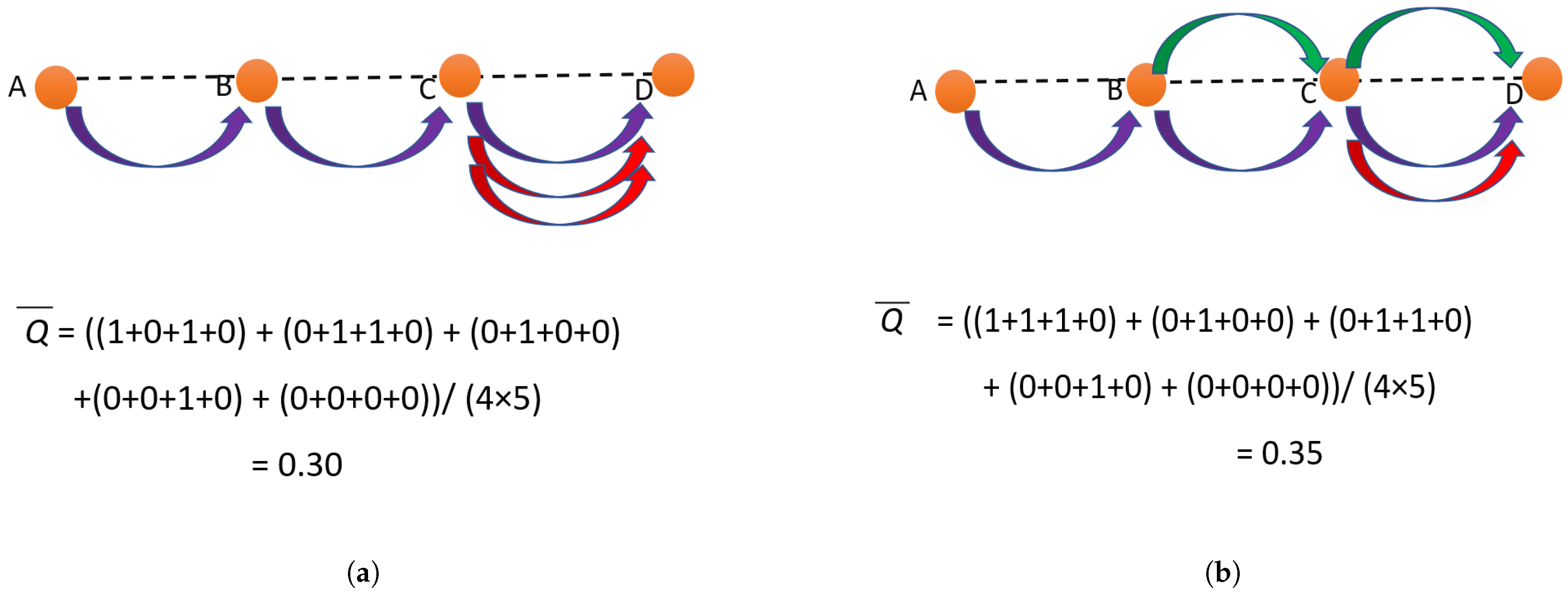
3.3.3. Computing Normalized Network Contention

Next, we numerically find the maximum of the average contention delay of wireless links by substituting ρ W L = 1 into Equation (23) to compute ( t c o n t , W L , m a x ¯ ), as in Equation (25):
t c o n t , W L , m a x ¯ = D I F S + C W m i n ( 2 ) E 3 T s l o t
Similarly, we can numerically find the maximum of the average contention delay of wired links by substituting ρ W I = 1 into Equation (24) to compute ( t c o n t , W I , m a x ¯ ), as in Equation (26):
t c o n t , W I , m a x ¯ = E × ( I F G + T c ) + C W m i n ( 2 ) E 2 T s l o t
Now we can define normalized wireless contention ( C W L ), as given in Equation (27):
C W L = t c o n t , W L ¯ t c o n t , W L , m a x ¯
Similarly, we can define normalized wired contention ( C W I ), as given in Equation (28):
C W I = t c o n t , W I ¯ t c o n t , W I , m a x ¯
Finally, we can formulate the normalized network contention ( C ) as a weighted summation of the normalized channel contention of each of the wired and wireless communication channels, as given in Equation (29):
C = N × C W L + N r × C W I N + N r
In Equation (29), N r is the total number of RSUs, and N is the total number of nodes. The composed knowledge of normalized network contention is used in deciding the mode of the hybrid link stability-based routing framework. Specifically, we distinguish high contention when C > 0.50 , and low contention otherwise.

3.3.4. Computing Average Per-Channel Delay at Each Hop

We can find the average value for propagation delay at the ith node ( t p r o p , i ¯ ) using Equation (30):
t p r o p , i ¯ = j = 1 N i D i j N i × v
In Equation (30), D i j is the transmission distance from node i to its jth neighbor, and v is the speed of signal propagation in the given medium.
Furthermore, in order to estimate the delay of each link, it is necessary to compute the average queue size of node i ( R i ¯ ), as shown in Equation (31):
R i ¯ = j = 1 M Y i j M
In Equation (31), Y i j is the queue size of node i at the jth time step, and M is the total number of time steps.
Finally, using the collected R i ¯ , computed t c o n t , W I ¯ , t c o n t , W L ¯ , and t p r o p , i ¯ , and Equations (11) and (12), the final delay equations can be formulated as given in Equations (32) and (33):
D i W L ¯ = R i ¯ × ( t t r a n s , i + 4 t p r o p , i ¯ + 4 t p r o c , i + t r t s + t c t s + t a c k + t c o n t , W L ¯ )
In Equation (32), D i W L ¯ is the average one-hop wireless link delay at node i using CSMA–CA.
D i W I ¯ = R i ¯ × ( t t r a n s , i + t p r o p , i ¯ + t p r o c , i + t c o n t , W I ¯ )
In Equation (33), D i W I ¯ is the average one-hop wired link delay at node i using CSMA–CD.
Thus, for each link that exists in the network, an average value for the link delay can be estimated using Equations (32) and (33). Note that the one-hop delays that are obtained from Equations (32) and (33) are only estimates for the average wireless or wired communication channel delay at the ith node and may not depict the exact delay that occurs at node i. The main reason for that is that the average contention delay for a given communication channel ( t c o n t , W I ¯ , t c o n t , W L ¯ ) is computed for the whole network, not for individual links. However, the average values obtained from Equations (32) and (33) can be used as very good initial estimates in deriving the exact delay per communication channel. In order to predict the exact delay, we use the concept of machine learning, as described below. Sample delay calculations using the above-derived Equations are given in Appendix B.

3.3.5. Predicting Exact One-Hop Channel Delay Using Machine Learning

We propose to use a DNN to predict the exact one-hop channel delay. The design choice of DNN for this regression task is discussed in detail in Section 5. Thus, for predicting the exact delay, the estimated average values for one-hop delay ( D i W L ¯ and D i W I ¯ ) can be provided as some of the inputs. There should be an input to select the mode (M) as wired (M = 0) or wireless (M = 1). The average queue size of node i ( R i ¯ ) should also be provided as one of the inputs. As pointed out earlier, the error, which is the difference between the estimates ( D i W L ¯ , D i W I ¯ ) and the real one-hop delay, occurs from the error in contention delay due to the average contention delay being a network global average. Thus, factors governing contention delay in a given hop should be investigated. The main factors which affect collision probability in a given hop ( ρ ) are similar to when it is derived for the whole network. These are listed below:
  • Number of links in the same communication channel connected to the hop ( N i W L or N i W I );
  • Average pending transmission packet distribution factor of the node and its neighbors ( Q i , n e i ¯ ), which can be calculated as given in Equation (34):
Q i , n e i ¯ = Q i ¯ j S i Q j ¯ N i ; i f N i > 0 ; 0 ; o t h e r w i s e .
In Equation (34), S i is the set of one-hop neighbors of node i, and N i is the total one-hop neighbors of node i.
Furthermore, there is an error due to obtaining the average value of the propagation delay ( t p r o p , i ¯ ). To compensate for any error that may occur in setting equal probability for selection of each path for propagation at node i, we input the maximum ( D i j , m a x ) and minimum ( D i j , m i n ) of link distances as inputs to the neural network, to fit the weights of the addition of maximum and minimum link distances to minimize the error.
Furthermore, there can be slight errors between the delays calculated for each individual delay component’s theoretical value and the practical value that occurs in the real network. For example, consider the transmission delay. We calculate transmission delay theoretically using t t r a n , i = p a c k e t s i z e / d a t a r a t e . However, the practical transmission delay can be slightly higher or lower than the theoretical value. Thus, to compensate for any error, we should input all input parameters for all average delay calculations in Equations (32) and (33) to the neural network. The following list summarizes the input parameters of the neural network to compensate for theoretical calculation errors:
  • Data packet size ( P D ), packet size of RTS ( P r t s ), packet size of CTS ( P c t s ), packet size of ACK ( P a c k ), and data rate (DR) to compensate for transmission delay errors;
  • Input Short Inter-Frame Space (SIFS) to compensate for processing delay errors;
  • E, T c , C W m i n , T s l o t , 1th–6th-order terms of ρ W L ¯ , and 1th–6th-order terms of ρ W I ¯ .
The DNN for predicting one-hop total delay per communication channel is graphically illustrated in Figure 10.
However, in high-contention scenarios ( C 0.5 ), the proposed algorithm’s metric is changed to distance, as the exact delay for choosing the least delay path is difficult to predict, even when using the exact delay prediction approach given above, due to the increment of randomness in the back-off approach in high-contention scenarios. Thus, there can be a large difference between the predicted delay and the practical one-hop delay that occurs in the network. However, in low-contention scenarios ( C < 0.5 ), the error between the value predicted by the neural network and the real one-hop delay that occurs in the practical network can be expected to be lower.

3.3.6. Computation of the Link Delay Matrix

Thus, under low contention scenarios, using the DNN to predict exact one-hop wireless delay ( D i W L ) and wired delay ( D i W L ) at each node, we can compute the link delay matrix ( D [ N , N , 2 ] ) containing link delays of each and every link of the network in both communication channels required for the routing algorithm, as shown in Equation (35):
D [ i , j , k ] = D i W L R i ¯ × ( 4 t p r o p , i ¯ + 4 t p r o p , i j k ) ; i f l i n k i j i s w i r e l e s s ( k = 0 ) D i W I R i ¯ × ( t p r o p , i ¯ + t p r o p , i j k ) ; i f l i n k i j i s w i r e d ( k = 1 ) 0 ; i f i = j l a r g e ; i f l i n k i j i n k t h c o m m u n i c a t i o n c h a n n e l d o e s n o t e x i s t
Note that, as evident from Equation (35), the delay for its own link D [ i , i , k ] is zero. In Equation (35), t p r o p , i j k is the propagation delay from the ith node to the jth node using the kth communication channel type. Note that, within the same communication channel, even for links existing between a given source node and different other nodes, a link delay difference occurs due to the propagation delay, which is very low. However, between different communication channels (wired and wireless), even from the same source node (i) to another given destination node (j), the link delay can be significantly different, as computed from the delay prediction machine learning model given in Figure 10.

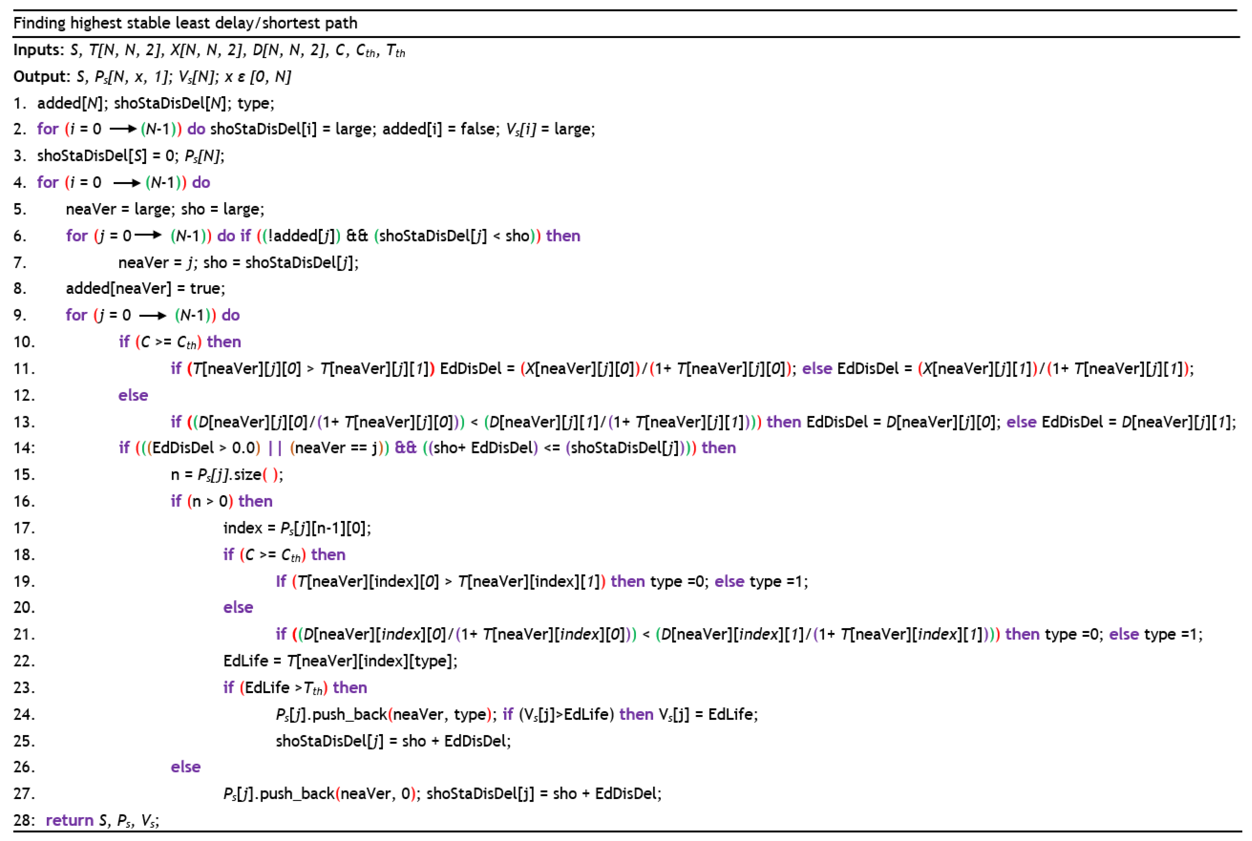
3.4. Hybrid Algorithm for Finding the Highest Stable Least Delay Path or Highest Stable Shortest Path

Let there be N nodes in the vehicular network. The algorithm finds the highest stable path (least delay or shortest path) from each and every other node to a given destination node. We find paths from each and every other node in the network rather than from a given source node for the following reason: in both cases, for finding a route from a given source node to a given destination and for finding routes from each and every node to a given destination node, the algorithm should run iteratively through all N nodes in the network to compute paths, as evident from Figure 1. It can be proven, using asymptotic runtime complexity analysis, that the total runtime complexity of finding N paths separately from a given source node to a given destination node by running the algorithm for N times is much higher ( O ( N 3 ) ) than computing paths from each and every node to a given destination node at once using a single algorithm run ( O ( N 2 ) ). Thus, the runtime complexity of the hybrid routing algorithm is O ( N 2 ) . Furthermore, the space complexity of the hybrid routing algorithm is also O ( N 2 ) . The controller workload is a key aspect of SDVN, as, when the number of nodes in the network increases, the workload of the controller increases, meaning that every effort should be made to reduce the computational complexity at the controller for any given solution to be scalable. Thus, we stick to the approach of finding routes from each node to the given destination vs. the computationally inefficient approach of finding a path from a given source to a given destination.
The choice of least delay or shortest path depends on the current normalized network contention value. The inputs to the algorithm are the destination node (S), adjacency matrix of link lifetime ( T [ N , N , 2 ] ), adjacency matrix of position ( X [ N , N , 2 ] ), adjacency matrix of estimated delay ( D [ N , N , 2 ] ) for two communication channels (wired and wireless), normalized network contention ( C ), link lifetime threshold ( T t h ), and network contention threshold ( C t h ). The diagonal elements of the adjacency matrices X, D, and T are zero, since the distance, delay, and lifetime from node to node are themselves zero. Furthermore, note that the link lifetimes and delays of non-existing links (inter-node displacement greater than the maximum wireless transmission distance for wireless links) are zero and large, respectively. The outputs are P s [ N , x , 1 ] , V s [ N ] , and the destination node S. P s [ N , x , 1 ] is an adjacency list containing paths (Node ID and link type to visit in arriving at destination node S) from each and every other node to destination node S, where x [ 0 , N ] . V s [ N ] is the path valid time vector, which contains the maximum time that each of the computed paths to destination node S is valid (the lifetime of each route). For instance, P s [ i , x , 1 ] and V s [ i ] contain the path and path valid time from source node i to destination node S, respectively. The pseudo-code for the hybrid algorithm for finding the stable least delay or stable shortest path is given in the code snippet in Figure 1.
The stable path-finding algorithm given in Figure 1 can be described as follows. “added” and “shoStaDisDel” are N-dimensional arrays. “type” is a variable to store the link type (communication channel type). “added” is used to track the already included vertices when finding the stable path. “shoStaDisDel” is used to store the stable shortest distance or stable least delay from the node represented by the ith array index of “shoStaDisDel” to the destination node. Line 2 of the algorithm initializes all “shoStaDisDel” elements with large integer values; the “added” array is initialized as false, as no elements are added to routes in the beginning. However, as seen in Line 3, it follows from logic that the sum of the stable shortest distance or stable least delay from the destination node to the destination node itself is zero. Next, a loop begins to iterate N times, whose purpose is to add the nearest vertex to paths leading to destination S from each source node. At the beginning of that loop, local variables “neaVer” and “sho” are initialized to large. “neaVer” is a variable used to track the nearest stable shortest distance or stable least delay vertex included in the “added” array for the last time. “sho” stores the total stable shortest distance or total stable least delay from the vertex finally added to the “added” array to the destination node. At the end of the for loop in Lines 6 and 7, the nearest stable vertex that has not yet been added to the path is found. In Line 8, the nearest stable vertex is added to the “added” array by setting the corresponding index to a true value. Next, another loop begins in Line 9, whose purpose is to iterate through all links from the finally added nearest stable vertex to all other nodes.
Using the composed knowledge on normalized network contention ( C ), the mode of the routing algorithm is decided by comparing the contention against a contention threshold ( C t h ), as given in the piecewise function in Equation (36):
R o u t i n g m o d e =   H i g h e s t s t a b l e s h o r t e s t p a t h r o u t i n g ; i f C > = C t h   H i g h e s t s t a b l e l e a s t d e l a y r o u t i n g ; i f C < C t h
The algorithm creates a local variable known as “EdDisDel”, which stores the highest stable least distance or link delay to the nearest vertex from the jth node. As evident from Lines 10 and 11 of Figure 1, if normalized network contention ( C ) is greater than or equal to the contention threshold ( C t h ), “EdDisDel” will store the highest stable least distance. Note that, in distance mode, in order to compute the highest stable least distance metric, we get obtain ratio of distance with link lifetime plus one (to prevent the metric from reaching infinity at zero link lifetimes). Thus, low link lifetimes will result in a higher value for the metric, and vice versa. In particular, we first inspect the link lifetimes ( T [ n e a r V e r ] [ j ] [ 0 ] and T [ n e a V e r ] [ j ] [ 1 ] ) and select the channel having the higher link lifetime in computing the highest stable least distance metric, as evident from Line 11. When the contention is lower than the threshold, delay mode will be selected. Then in delay mode, “EdDisDel” will store the highest stable minimum delay to the nearest vertex from the jth node in the kth communication channel, where “EdDisDel” is selected by considering the combined effect of link delay and lifetime, as evident from Line 13. For example, consider the links between two RSUs, where there is each a wireless link and a wired link. Then, using the delay matrix ( D [ n e a V e r ] [ j ] [ k ] ) and link lifetime matrix ( T [ n e a V e r ] [ j ] [ k ] ), the link having the combined effect of least delay and highest stability (the combined effect is computed by obtaining the ratio of D and T) out of wireless and wired communication channels will be chosen as “EdDisDel” for further processing, as evident from Line 13 in Figure 1.
The if-condition in Line 14 checks whether the edge distance or delay (“EdDisDel”) is greater than zero, the nearest vertex (“neaVer”) is equal to the source index (j), or the sum of the distances or delays from the nearest stable vertex (“sho”) plus edge distance or delay is less than or equal to the current stable shortest distances or stable least delays from the jth node (“shoStaDisDel[j]”). Note that, when the nearest vertex is equal to j, the above if-condition is satisfied, even though “EdDisDel” is equal to zero in that scenario. Next, the size of the route to reach the jth node is set to “n”, as evident from Line 15. If the route size is zero, then the destination node with default link type 0 should be added to the route, and the stable shortest distance or stable least delay from the source (jth) node to the destination node should be updated, as shown in Line 27 of the code snippet given in Figure 1. The default link type is added as zero because there is no link in the route with destination being the only element; note that this link type is not used in decision-making. Thus, P s [ j , 0 , 0 ] does not represent any link type in the path, while all other elements in the path indeed represent link types, including the source node. Accordingly, P s [ j , 0 , 0 ] is a dummy link type. Otherwise, if the size is greater than zero, the last parent from the stable route to the jth node will be set as “index”, as evident from Line 17. Then, it is necessary to determine the link type that exists between “neaVer” and “index”. For that, we have to inspect the link type in one of the stable least distance or stable least delay modes. Note that “type” is a variable that holds the type of communication channel for the link between “neaVer” and “index”. If the mode is distance, then the communication channel having the highest link lifetime will be selected, as evident from Lines 18 and 19. Otherwise, if the mode is delay, the combined effect of link lifetime and delay will be inspected, as specified previously, to select the communication channel “type” with the combined effect of low delay and high link lifetime, as evident from Lines 20 and 21. Link lifetime checks in both distance mode and delay mode ensure that the most stable links out of the two communication channels are selected, ensuring higher reliability in routing.
Next, “EdLife” is a local variable which stores the link lifetime from the nearest vertex to the last parent of the route from the jth node (“index”) in the communication channel “type”, as evident from Line 22. The if-condition in Line 23 checks whether the link lifetime of the edge (from the nearest vertex to the last element of the parent vector containing a stable least distance or least delay path from the jth node: “EdLife”) is greater than the link lifetime threshold ( T t h ). Note that the previous if-condition is satisfied if and only if there is a stable link from the nearest vertex to the last parent of the path containing the route from the jth node to destination node S. Therefore, if that condition is true, the nearest vertex with the corresponding link type will be added as a parent to the stable route having the source as the jth node, as evident from Line 24. Furthermore, when a link is added to the path, the route valid time should be updated. If the added edge’s link lifetime (“EdLife”) is less than the present path valid time ( V s [ j ] ), then the value of V s [ j ] should be updated as “EdLife”, as shown in Line 24. Next, the total stable shortest distance or total stable least delay from the jth node (“shoStaDisDel[j]”) is updated as the distance or delay from the nearest stable vertex (“sho”) plus edge distance or delay (“EdDisDel”), as evident from line 25. Therefore, this approach ensures that only the nearest stable vertices with link types are added to the adjacency list P s [ j , x , 1 ] , which contains a list of parent nodes and link types to choose from, in order to traverse from the source node “j” to the destination node S. At the end of the algorithm, the adjacency list P s [ N , x , 1 ] and path valid time vector V s [ N ] are returned, as given in line 28 of Figure 1. Note that all the routes in the adjacency list P s [ N , x , 1 ] are guaranteed to be free from routing loops, since an already added vertex will not be added to the route again, which is achieved by tracking added vertices using the “added” vector, as explained in the algorithm.
Table 2 summarizes the notations used in the proposed routing framework.

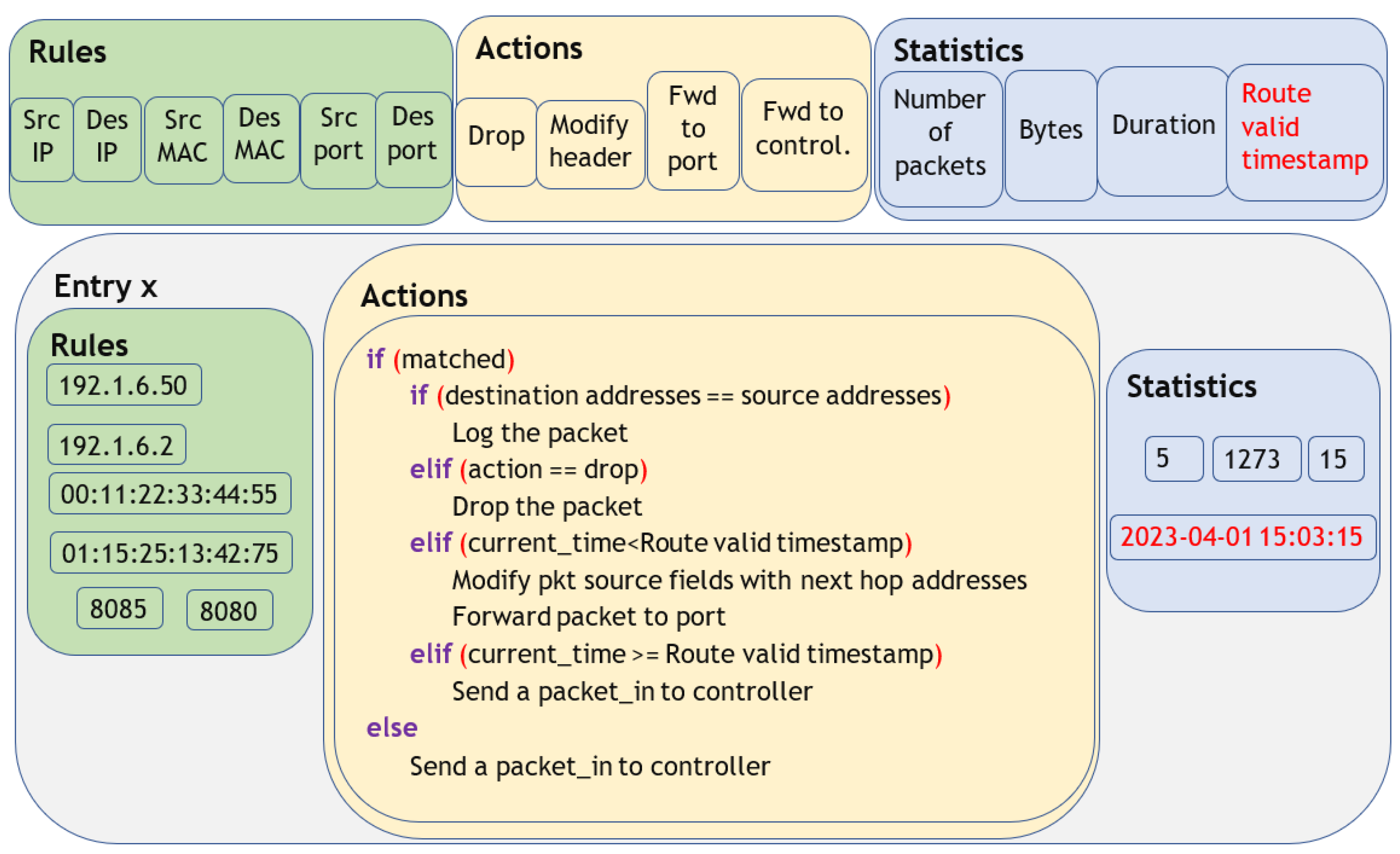
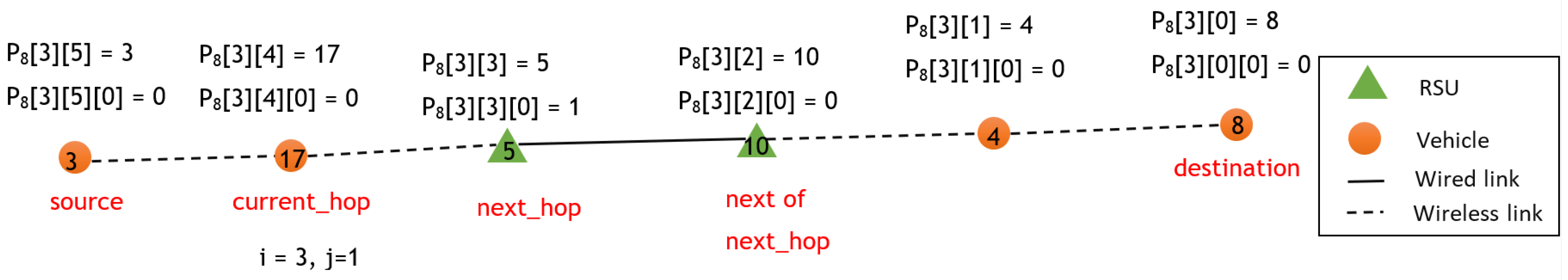
3.5. Proposed Flow Table Architecture

OpenFlow is the most widely used protocol for the southbound Application Programming Interface (API) of SDN, which can be used to install flow rules in switches. We propose our routing framework to be compatible with the current OpenFlow protocol. A flow table in the OpenFlow protocol necessarily consists of a set of rules to match incoming packets (source and destination addresses), a set of instructions to undertake upon receiving a match, and statistics for the particular flow, such as the number of packets, number of bytes, flow duration, etc. In order to incorporate reactive flow rule installation for the proposed routing framework, we propose to use the flow table architecture given in Figure 11, where we have shown the architecture and a sample entry that is compatible with the existing OpenFlow protocol flow table.
As evident from Figure 11, the key component that we propose to include as a statistic in the flow table is the route valid timestamp. The route valid timestamp for the path from source node j to destination node i is computed by the controller by using the V i [ j ] returned from the routing algorithm and adding it to the present timestamp. However, at the switch, for a given matched packet whose source and destination addresses are the same, it means that packet has reached the destination, so that packet will be logged, as shown in Figure 11, irrespective of the route valid timestamp. Otherwise, for a matched packet, if the drop action has been explicitly defined by the controller, then the packet will be dropped. Such a drop action will be defined by the controller when there are no existing routes from a given source to a given destination (e.g., if the destination is a node that is not known by the controller). For a matched packet with a present route timestamp less than route valid time whose destination and source addresses are not the same and action is not explicitly defined as drop, then the first packet’s source fields will be modified with the next hop addresses, and then the packet will be forwarded to the next hop using the given communication channel (by forwarding through the appropriate source port), as shown in Figure 11. Otherwise, for a matched packet, the packet will not be forwarded, and the switch will send a packet-in message to the controller, requesting to send a valid route from the given source to destination as the current path in the flow table is no longer valid. The current path is no longer valid when the present time exceeds the route’s valid timestamp in the flow table because one or more links’ lifetimes in the present path have expired due to the mobility of the nodes. Thus, by including the field route valid timestamp as a statistic in the flow table, we successfully prevent packet forwarding on expired paths. Furthermore, a packet_in message will be sent to the controller if a flow table match is not found, as shown in Figure 11. Note that this approach reduces communication overhead, as the controller is consulted only when a given path expires or when a flow-table mismatch occurs (when the switch is unaware of actions to undertake for the packet). Therefore, the key novel aspect in the architecture of the proposed flow table is that, due to the inclusion of the “route valid timestamp” field in the flow table, the controller is contacted to update the switch with the latest flow rules when the existing path in the switch for a matched packet has expired.

3.6. Flow Table Update at the Controller

Routing algorithm finds either the highest stable least delay path or the highest stable shortest path from each and every other node to a given destination node. Thus, the outputs of routing algorithm are the adjacency list of computed paths ( P s [ N , x , 1 ] ), destination node (S), and path valid time vector V s [ N ] . The controller maintains a topology database at the controller that stores the topology of the network, consisting of Node IDs, IP addresses, MAC addresses, port addresses, location, velocity, acceleration, etc. Note that node ID is a node index maintained by the controller to distinctly identify each node easily, which ranges from 0 to N 1, where N is the total number of nodes in the network. We collect these data as status data by unicasting from agent nodes, along with the metadata required to compute other parameters for routing to the controller, using a data collection optimization framework for SDVNs that we have proposed in one of our previous research works (elucidated in Appendix A). For a given node, there are two sets of IPs, MACs, and port addresses. Vehicular nodes have a DSRC interface (which we represent using index 0) and a cellular interface (which we represent using index 1). RSU nodes have a DSRC interface (represented by index 0) and a wired interface (represented by index 1).
The purpose of the flow table update algorithm is to update all flow table entries when P s [ N , x , 1 ] , V s [ N ] , and S are given, which are the inputs to the algorithm. It can be proven, using asymptotic complexity analysis, that the runtime complexity of flow table update algorithm is O ( N ) , while the space complexity is O ( N 2 ) . There is no output for this algorithm. The pseudo-code in Figure 2 depicts the operation of the proposed flow table update algorithm at the controller.
As evident from Line 1 in Figure 2, variable “next_hop” tracks the next hop ID, “current_hop” tracks the source node ID, “current_hop_link_type” tracks the type of the link (wired—1 or wireless—0) which exists between source node to next hop, “next_hop_link_type” tracks the link type which exists between the next hop and the further next hop of the current next hop, “destination_link_type” tracks the link which exists between the hop before the destination and the destination node, “valid_time” tracks the route valid time, and, finally, “visited” array tracks the source nodes that already updated the flow table to prevent multiple updating of the same source node. Initially, the “visited” array is initialized to false, as none of the routes have been updated, as evident from Line 2. Note that the for loop that starts on Line 3 visits each path of the parent vector P s [ N , x , 1 ] indexed by integer i, while the purpose of the for loop in Line 6 is to iterate on each path of the parent vector indexed by integer j.
First, the size of the path from node i to destination node S is assigned to the variable “size”, as shown in Line 4. Note that there may not be a stable route from a given source to a given destination. When there is no stable path, the output path from the routing algorithm will definitely not contain the source node as the last element of the path. Thus, in Line 5, we check whether the source node ID exists in the last element of the path and whether the source node ID is not equal to the destination node ID. When this if-condition is false, it means that either source node ID and destination node ID are the same or that there is no stable path from source node i to destination node S. In that case, the flow table can be immediately updated to drop or log the packets. Note that “Map_all” is a function to map all addresses related to a given Node ID using the topology database at the controller. In Lines 22 and 23, all source addresses (“src_node_addresses”) related to source node ID i will be mapped, and all destination addresses related to destination node S are mapped to the variable “destination_addresses”. Note that “Update_flow_table_log” is a function that updates the flow entry having destination and source addresses with “src_node_addresses” with the action “log the packet”. This logging is defined for flow table entries having the same source address and destination address, as evident from Lines 24 and 25. Note that “Update_flow_table_drop” is a function that updates all flow entries matching source addresses and destination addresses provided as input to the function with the action “drop the packet”. Thus, in Lines 26 and 27, “Update_flow_table_drop” with input arguments “src_node_addresses” and “destination_addresses” will update flow table entries matching those address pairs with the action field set to “drop”.
However, when the if-condition in Line 5 is satisfied (when there is a stable path from source i to destination “S” with different source and destination IDs), the path will be inspected and the flow table will be updated with action conditional forwarding. We call this conditional forwarding, as the forwarding will occur if and only if the path valid timestamp is greater than the current timestamp. Otherwise, a “packet_in” message will be generated. The “current_hop” is set as P s [ i ] [ s i z e 1 j ] , as evident from Line 7, which will be the last element of the path when j = 0 and will dynamically become the next hop when the value of j is incremented. Line 8 sets the “current_hop_link_type” using the corresponding channel type of the current hop ( P s [ i ] [ s i z e 1 j ] [ 0 ] ). Line 9 checks whether “current_hop” has already been updated in the flow table or not. If it is already updated, no changes are made; otherwise, it proceeds with updating.
Setting the next hop addresses is the trickiest part because there are mainly two types of links: wireless (DSRC) and wired (Ethernet) for routing. Let us understand this using an example route. Figure 12 shows a routing path represented by the parent vector P 8 [ 3 ] .
As shown in Figure 12, consider the situation when i = 3 ,   j = 1 , such that “current_hop” is a node with ID equal to 17, so that source packet will be forwarded from node 17 using the DSRC communication channel. However, if the flow table is modified such that next hop addresses correspond to the wireless communication channel, then, once it arrives on node 5, it will be dropped, as that node will not have a flow table entry with next hop as a node ID equal to 10 in the wireless communication channel. However, node ID equal to 5 will have an entry for the wired communication channel. Therefore, the communication channel for the next hop should be set by identifying the communication channel that exists between the next hop and the next of next hop. In this example, the next hop’s communication channel should be selected as Ethernet.
The if-condition in Line 10 checks whether the next hop is the last hop or not, and if it is not the last hop, “next_hop” will be assigned from the parent vector P s [ i ] [ s i z e 2 j ] and the corresponding “next_hop_link_type” will be selected ( P s [ i ] [ s i z e 2 j ] [ 0 ] ), as evident from Lines 10 and 11. Otherwise, if the next hop is the last hop of the path, then “next_hop” will be set as S and “next_hop_link_type” will be set as the “current_hop_link_type”, as there is no link after the destination, as evident from Lines 12 and 13.
Line 14 sets the “destination_link_type” by inspecting the parent vector P s [ i ] [ 1 ] [ 0 ] , and “valid_time” is set as the valid time of the current path, which is held by V s [ i ] in Line 15. The function “Map(ID, link_type)” maps node ID and link type with IP address, MAC address, and port address using the topology database available at the controller. Thus, in Line 16, source node addresses (“src_node_addresses”) are mapped using the current hop ID (“current_hop”) and link type between the current hop and the next hop (“current_hop_link_type”). Thus, the packet will be forwarded through the communication channel that exists between the current hop (the source node) and the next hop.
The addresses of the next hop to be modified as the source header fields before forwarding the packet depend on the link type that exists between the next hop and the next hop of the next hop. Thus, Line 17 maps the next hop’s addresses (“next_hop_addresses”) corresponding to the next hop ID (“next_hop”) and the communication channel that exists between the next hop and the next hop of the next hop (“next_hop_link_type”). The algorithm also inspects the destination node ID (“S”) and the link type that exists between the hop before the destination and the destination (“destination_link_type”), and maps the corresponding addresses from the topology database at the controller to retrieve “destination_addresses”, as evident from Line 18 of Figure 2.
Then, the flow table is updated to conditionally forward the packet using the “Update_flow_table_conditional_forward” function, as shown in Line 19. It updates source node addresses (“src_node_addresses”) and destination addresses (“destination_addresses”) for the rules field of the flow table. Next hop addresses (“next_hop_addresses”) will be set as an instruction in the action field to conditionally forward a packet through the source port if the route valid timestamp is greater than the present timestamp, and, if not, send a packet_in message to the controller, and the route valid timestamp will be set by adding the current timestamp to the ”valid_time“. Finally, the element of the “visited” array corresponding to “current_hop” will be set as true, as shown in Line 20, to mark in the flow table related to “current_hop” that the source node and destination node S have already been updated and are not required to be updated again.

3.7. Adaptive Flow Rule Computation, Update, and Installation

OpenFlow can use both a proactive approach (the controller pre-computes routes and installs flow rules in switches) and a reactive approach (upon finding a flow table mismatch, it switches request routes from the controller, which will respond with computed routes reactively) [63]. One trivial way to use the proposed routing framework is to use a proactive routing approach. However, the proactive approach consumes more controller workload and results in high communication overhead between the controller and switches, making it a less scalable approach compared to the reactive approach [64]. Conversely, in the initial cycle, as all switches are unaware of flow rules, using a reactive approach for the first cycle can cause more overhead, even though the controller workload is the same. Therefore, we propose to use proactive flow rule installation for the first cycle of routing and an adaptive approach for all the cycles. We call this approach adaptive, as it is not completely reactive, which means that flow rules are not computed for each packet_in message. This is because it is not necessary to compute the routes using the routing algorithm and update flow table entries using the flow table update algorithm each and every time a packet_in is received at the controller, because this can unnecessarily exhaust the controller. Thus, we propose an algorithm for adaptively computing routes, updating flow rules, and creating a FlowMod message for flow rule installation in the switches, as shown in the flowchart given in Figure 3.
As evident from the flow chart shown in Figure 3, upon reception of a packet_in message, it is first verified whether the source and destination nodes are known by the controller or not. If either source or destination are unknown, a FlowMod packet will be constructed with action set to drop in order to instruct the corresponding switch to drop the packet. Otherwise, if both source and destination are known by the controller, then the flow table residing at the controller will be matched using the source and destination addresses of the packet_in message, and the route valid timestamp of the matched entry will be inspected. In case the flow table entry’s route valid timestamp is less than the current timestamp, meaning that the flow table entry’s route has expired, then only new routes will be computed using the routing algorithm by setting the destination node as a particular destination, and then the flow table will be updated using the flow table update algorithm. When a flow table route to a particular destination is expired, the adaptive flow rule computation and update algorithm will update the flow table entries of all routes whose destination is the destination of the packet_in message. This makes sense, as, when the link lifetime of a given link in a routing path to a given destination is zero (expired), it is likely that many other paths leading to the given destination have also expired. Thus, when a packet_in message comes from such other expired paths leading to the particular destination, it is not necessary to compute paths using the routing and flow table update algorithms again because those paths have already been updated in the flow table using only one run each of routing algorithm and flow table update algorithm. When a packet_in message comes from switches for expired paths (at the switches), if the flow table entry route valid timestamp is greater than the current timestamp for the path (due to previously updating the flow entry for a previous packet_in message leading to the same destination), a FlowMod packet can be immediately created without running routing algorithm and flow table update algorithm. Therefore, this algorithm is an adaptive flow rule computation, update, and installation approach.

3.8. Overall Routing Process

We assume that all routing takes place in the data plane only, which uses DSRC (wireless) and Ethernet (wired) communication for routing. Cellular (V2I, I2V) links are not directly utilized for routing, even though, in SDVN, they are utilized for metadata collection, for subsequent computations, to make routing decisions, and to unicast computed flow rules from the controller to the switches. We chose the optimum link lifetime threshold ( T t h ) for routing algorithm after a performance analysis. The process of metadata collection for routing, parameter computation, route finding, flow table updating, and routing scheduling in each routing cycle for the proposed routing framework is graphically illustrated in Figure 13 and listed below:
  • We use the data collection optimization model proposed in our previous work [65] for metadata collection for the routing framework. Metadata refers to all data, namely, status data (node addresses, position, velocity, acceleration), node address set of all one-hop neighbors of each node ( S i ), average pending transmission packet distribution factor of each node ( Q i ¯ ), and average queue size of each node ( R i ¯ ), which are required to compute the routes using the proposed hybrid routing algorithm given in Section 3.4. However, in the very first routing cycle, as routing has not taken place at least once, Q i ¯ and R i ¯ cannot be collected, and only status data and S i are collected, as shown in block ”U0“ in Figure 13. These metadata are unicasted to the controller node from the agent nodes in the data collection optimization model. In the initial routing cycle, only X [ N , N , 2 ] and T [ N , N , 2 ] are computed at the controller node, as shown in block ”K0“ in Figure 13. X [ N , N , 2 ] (the adjacency matrix of position) is computed using the position data of all nodes, while T [ N , N , 2 ] is computed using Equation (5) with the aid of the wireless link lifetime prediction DNN by providing differential position, velocity, and acceleration to the machine learning model, as described in Section 3.2. In the very first routing cycle, D [ N , N , 2 ] cannot be computed, as data do not exist for R i ¯ and Q i ¯ . Furthermore, it is not necessary to compute other parameters that are required to compute normalized network contention ( C ), as data do not exist to compute the average pending transmission packet distribution factor of the network ( Q ¯ ). Because of this, in the very first routing cycle, the value of C is assumed to be one, to utilize the highest stable least distance as the mode for the routing algorithm given in Section 3.4;
  • In the initial cycle, once X [ N , N , 2 ] and T [ N , N , 2 ] are computed, routes are computed using the hybrid routing algorithm by choosing stable distance as the metric, and the output of this algorithm is fed to flow table update algorithm to update flow table entries. Routing algorithm can compute only routes from all other nodes to a given destination node, so routing algorithm and flow table update algorithm should be executed iteratively N times, where N is the total number of nodes, by varying the destination node ID, to find routes from each and every source node to each and every destination node, as shown in block “Z0” in Figure 13. Using the parent vector, path valid time vector, and destination node ID output from routing algorithm, flow table update algorithm updates flow table entries. This updating of the flow table by flow table update algorithm occurs at the end of each iteration of finding routes by routing algorithm. At the end of the functioning of block “Z0” (once the updating of the flow table is over), the controller must unicast FlowMod packets related to each flow entry of the flow table to corresponding switches, as shown in block “B1” of Figure 13;
  • Routing occurs at a routing frequency (f), and, at each routing cycle, including the very first, routing occurs as packet transmissions are scheduled, as is evident from block “A” in Figure 13. Packets are forwarded through each node by inspecting the flow table of the node. Because of the implementation of route valid timestamp in the proposed flow table, when a flow table match occurs with source address not equal to destination address, action not explicitly defined to drop, and current timestamp greater than the route valid timestamp, a packet_in message will be generated and sent to the controller, as shown in block “C1” in Figure 13, as the current flow entry in the flow table at the switch has expired. Then, in response to the packet_in message, the adaptive flow rule computation, update, and installation algorithm will run as shown in block ”C2” in Figure 13 to create a FlowMod packet containing flow modification rules, which will be unicasted to the corresponding switch, as shown in block “C3” in Figure 13, to update the corresponding flow table entry in the switch with updated flow rules. Note that, if a flow table mismatch occurs due to a packet scheduled to a destination node that does not exist in the vehicular network, a packet_in message will be sent to the controller. Then, the adaptive flow rule computation and update algorithm will inspect the destination, and, as it does not exist in the topology database, a FlowMod packet to drop the packet at the switch will be sent back to the switch. During the entire routing time period (the time period during which routing occurs), each node monitors its transmission queue size at discrete time intervals and computes the parameters’ average queue size ( R i ¯ ) and average pending transmission packet distribution factor ( Q i ¯ ), as shown in block “K1” of Figure 13. Computed R i ¯ and Q i ¯ values are kept with the nodes until they are unicasted to the controller node in the next routing cycle, along with other metadata, as shown in block “U1” of Figure 13. The routing in all routing cycles is similar (Functioning blocks “K1”, “A”, ”C1”, “C2”, and “C3” operate in each routing cycle, including the initial cycle, similarly);
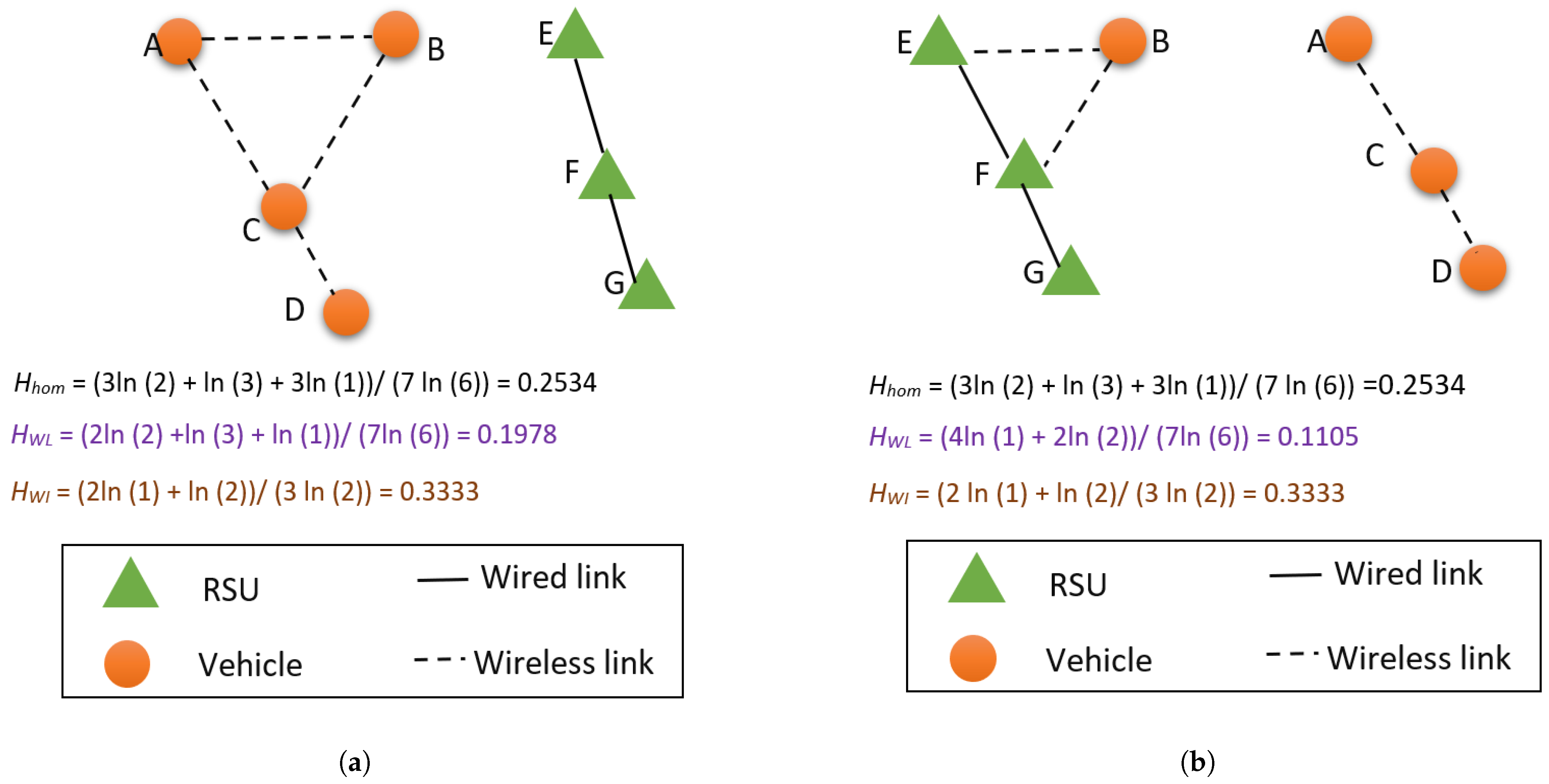
  • Starting from the second cycle (subsequent cycle 1) onwards, agent nodes should collect and unicast status data, a set of node addresses of one-hop neighbors of each node ( S i ), R i ¯ , and Q i ¯ computed from the previous routing cycle, as evident from the “U1” block in Figure 13. Thus, at the controller node, Q ¯ is computed using the Q i ¯ values received from all the nodes. X [ N , N , 2 ] and T [ N , N , 2 ] are computed at subsequent routing cycles in the same manner specified for the initial cycle. Furthermore, starting from subsequent cycle 1 onwards, normalized homogeneous link entropy with respect to wireless links ( H W L ), normalized homogeneous link entropy with respect to wired links ( H W I ), average collision probability for wireless links ( ρ W L ¯ ), average collision probability for wired links ( ρ W I ¯ ), and average contention delay for wired links ( ρ W I ¯ ) are computed, as shown in block “K2” of Figure 13. Using previously computed parameters, normalized network contention ( C ) is computed using Equation (29). Furthermore, the adjacency matrix of link delay ( D [ N , N , 2 ] ) can be found using Equation (35), with the help of the one-hop per-channel delay prediction DNN. Descriptions of the computation of the above parameters are described in Section 3.3;
  • Once the link delay matrix ( D [ N , N , 2 ] ) and normalized network contention ( C ) are found, the routing algorithm will choose the mode as highest stable least distance or highest stable least delay by comparing C with C t h . However, unlike the initial cycle, routes will be computed, and flow table entries will be updated using the adaptive flow rule computation and update algorithm only upon reception of packet_in messages. As was described in the explanation of that algorithm, each packet_in message may not result in computing and updating the flow table at the controller. If the flow table entry corresponding to the packet_in message is already updated, that entry will be sent to the corresponding switch to update its flow table using a FlowMod packet.

4. Results

4.1. Performance Evaluation Metrics

In this research, we evaluated the routing performance of different routing techniques and the performance of wireless link lifetime prediction and one-hop channel delay prediction machine learning models, using the following performance evaluation metrics.

4.1.1. Root Mean Squared Error (RMSE)

As the wireless link lifetime and one-hop channel delay prediction using the DNNs are modeled as regression problems, RMSE is used as the performance evaluation metric, and it is computed as given in Equation (37) [66]:
R M S E = i = 1 N ( ( T i ) 2 ( T ^ i ) 2 N )
In Equation (37), T i is the true wireless link lifetime/one-hop channel delay of the ith sample, T ^ i is the wireless link lifetime/one-hop channel delay of the ith sample predicted by the machine learning model, and N stands for the total number of samples. A lower value for the RMSE is desirable.

4.1.2. Average Computational Time ( T c o m )

For wireless link lifetime prediction, we compute the average computation time per data gathering cycle ( T c o m ) using Equation (38):
T c o m = 1 K m = 1 K i = 1 N l i n k s T i
In Equation (38), T i is the computational time for predicting the wireless link lifetime of the ith link in the network, N l i n k s is the total number of wireless links in the network at the mth data gathering cycle, and K is the total number of data gathering cycles. A lower value for the T c o m is desirable.

4.1.3. Average Communication Cost ( C ¯ )

The mean of the total communication costs of all the nodes for all data collection cycles, as provided in Equation (39), can potentially be used to calculate the average total communication cost per node per routing cycle ( C ¯ ). A lower value of C ¯ shows that the method used to acquire the data results in an average reduction in communication costs.
C ¯ = 1 K N m = 1 K i = 1 N j = 1 L C j P i j
K is the total number of data collection steps, N is the sum of nodes, and L is the sum of communication channels utilized by the ith node in Equation (39). Subscript i denotes the node index, j is the channel index utilized by the ith node, and subscript m denotes the mth data collection cycle. P i j is the total packet size for sending a packet from the ith node using the jth communication channel, and C j indicates the communication cost per byte for communicating using the jth communication channel.

4.1.4. Average Channel Utilization ( U ¯ j )

Equation (40) could perhaps be used to obtain the average channel utilization for the jth communication channel ( U ¯ j ). The level of a particular communication channel’s occupancy is measured by channel utilization. When the channel usage score is high, it means that the network uses the channel frequently. A lower number for channel usage is preferred.
U ¯ j = 100 K m = 1 K t o t a l c h a n n e l u t i l i z a t i o n t i m e p e r d a t a c y c l e t o t a l t i m e o f t h e d a t a c y c l e
The quantity K in Equation (40) denotes the sum of data collection cycles.

4.1.5. Average End to End Latency ( T ¯ )

Equation (41) is used to compute the average end-to-end latency for each node during a data collection cycle ( T ¯ ). A packet’s latency is the amount of time it takes to travel from its source to its destination. The ideal latency value is minimal.
T ¯ = 1 K m = 1 K 1 N d i S d ( T r i T s i )
The receiving timestamp of the packet sent by the ith node at the destination is T r i in Equation (41), whereas the sending timestamp of the packet sent by the ith source node is T s i . In addition, N d is the total number of delivered packets in a routing cycle, S d is the source node ID set of delivered packets, and K is the total number of data collection cycles. The data packets are routed between the nodes (OBUs or RSUs). Therefore, the end points (source and destination) for latency calculation are two different nodes (two data plane units).

4.1.6. Average Packet Delivery Ratio ( R )

The ratio of delivered packets to total packets sent, or the packet delivery ratio ( R ), is used to gauge a system’s reliability. It is preferable for R to be close to unity. The average packet delivery ratio is determined using Equation (42):
R ¯ = 100 K N m = 1 K i = 1 N X r i X t i
In Equation (42), X r i is the total number of packets received at corresponding destinations that are sent from source node i; X t i is the total number of packets sent from source node i; K is the total number of data gathering cycles; and N is the total number of nodes. As was specified for latency, the source and destination for R ¯ computation are also two different nodes (OBUs or RSUs). The meaning of the average Packet Delivery Ratio (PDR) given in Equation (42) in routing is the reliability of the routing framework in delivering packets from a given source node to a destination node on average.

4.2. Configuration of the Simulation Environment

Using Network Simulator 3 (NS3) 3.35, we simulated the vehicular network. NS3 is constructed as a Linux computer and uses the C++ programming language. It has internal interfaces and application interfaces that are more realistic than those of its competitors [67]. As a result, the NS3-based modeling of vehicular networks is realistic and accurate.

4.2.1. Configuration for Routing

Ad Hoc On-demand Distance Vector (AODV) is a reactive routing protocol that is used in distributed VANETs in which routes are obtained on demand [68]. Dijkstra’s algorithm, which is a shortest path-finding algorithm, has been used as a routing algorithm for SDVN [69]. Thus, we used Dijkstra’s algorithm for routing in SDVN and AODV for VANET, in order to test the effectiveness of the proposed routing framework for the SDVN paradigm.
Configuration of Wireless Link Lifetime and Channel Delay Prediction Model
For wireless link lifetime prediction using optimization, we used GuRoBi commercial optimizer version 10.0.0 as the optimization tool. A comparative analysis that compared GuRoBi to other commercial optimization solvers such as CPLEX and XPRESS revealed that GuRoBi provides fast solutions due to its support for different optimization problems, multi-threading capability, and automatic linearization of problems [70]. We implemented the optimization model using a Python script, where we used the GuRoBiPi Python library to find the link lifetimes.
As the transmission power of a DSRC network device at a given node is variable (33 dBm for an urban scenario; 41 dBm for a rural scenario; 44 dBm for an autobahn scenario), the maximum transmission distance of a given wireless link ( D i j m a x ) is also variable in the network. We spawned 100 RSU nodes and 100 vehicle nodes in pairs and moved each vehicle node away from the RSU in the x direction, from where the vehicle node broadcasts its position to the RSU. When the RSU no longer receives broadcasts from the vehicle node, the difference between the x coordinate of the RSU node and the last received broadcast is computed as the maximum transmission distance. In this manner, for each of the mobility scenarios, the mean and variance of the maximum wireless transmission distances for the 100 pairs are calculated. Thus, the D i j m a x required for finding the link lifetime was modeled as a normal distribution with a mean and variance calculated as above. Note that there were three sets of normal distributions of D i j m a x for each of the mobility scenarios. Accordingly, it was experimentally found that the mean and standard deviation of the maximum transmission distance for the urban scenario are 156.1 ± 0.3 m, the rural scenario are 270.4 ± 0.5 m, and the autobahn scenario are 332.3 ± 0.7 m.
For collecting data sets for wireless link lifetime and one-hop channel delay prediction neural network training and testing purposes, we created a network having 100 vehicle nodes and 50 RSUs for each of the mobility scenarios, with 60 km/h as the maximum speed of vehicles for urban mobility, 100 km/h as the maximum speed for rural mobility, and 250 km/h as the maximum speed for the autobahn mobility scenario. If the neural networks are trained using only the data collected from a single vehicular network, there can be a bias in the data set, as the data are not uniformly distributed in their range of values in a given vehicular network. Data set bias can cause inaccurate training and over-fitting. Thus, in order to have a uniform distribution of training data, we obtained data from three different mobility scenarios with different maximum velocities in the network.
Collecting a data set for wireless link lifetime prediction—A similar approach to finding maximum transmission distance was used for obtaining wireless link lifetimes and status data from the vehicular network, which are used to train the wireless link lifetime prediction DNN. In particular, we scheduled broadcasting of status data (timestamp, node addresses, position, velocity, and acceleration) at 1 kHz frequency, where the received node stored the received status in the specific position of a 100,000 size data structure corresponding to 100,000 samples for 100 s. Note that wireless link lifetime of each sample in the data structure was the time elapsed from the timestamp at which the sample was received up to the timestamp at which reception of status from the given node address stopped (as the link has ceased to exist), or timestamp at the passage of 100 s in the case where the link continued to exist. Thus, when reception of status data from a given node stops or at the passage of 100 s, we stored (appended) the destination and source node’s position, velocity, and acceleration along with the wireless link lifetimes for all samples stored in the data structure in a CSV file. Thus, we collected a combined data set having 3,368,564 samples for wireless link lifetime prediction training and testing.
Collecting a data set for one-hop channel delay prediction— R i ¯ , Q i ¯ , and S i of each node were collected and updated in the control node of the SDVN architecture, where data were collected at a 1 Hz frequency. Specifically, for generating a well-distributed data set in terms of input variables for one-hop channel delay prediction, we generated different data sets by varying the packet sizes in the set [10, 100, 1000] bytes, the DSRC data rate in the set [6, 12, 27] Mbps, the Ethernet data rate in the set [10, 100, 1000] Mbps, T s l o t in the set [20, 40, 60], and E from 1 to 6 by varying C W m i n ,   C W m a x in the range 15 to 1031. Input data (1 × 30) required for one-hop channel delay prediction and the corresponding one-hop channel delay were saved in a CSV file to be read by a Python script for training. Note that the one-hop total delay for each hop in the network for each of the communication channels was computed by monitoring each packet’s sending and receiving timestamp values in each of the communication channels. Specifically, for a given hop (i) in a given communication channel, the timestamp difference refers to the difference between the receiving timestamp of the last packet at the destination sent from node i through the given communication channel and the sending timestamp of the first packet from the given hop (i) in the given communication channel. The one-hop wired channel delay in CSMA–CD ( D i W I ) directly precedes the timestamp difference, whereas, for CSMA–CA, the total one-hop wireless channel delay ( D i W L ) can be obtained by adding t p r o p , i + t p r o c , i + t a c k to the preceding timestamp difference. We collected two sets of one-hop delay data sets consisting of 3,500,000 samples each for low-contention ( C < 0.5 ) and high-contention scenarios ( C 0.5 ).
Pre-processing of the data sets—The wireless link lifetime data set collected cannot be directly fed into the DNN. The wireless link lifetime data set needs to be pre-processed before feeding into the DNN. As the first pre-processing step, from the collected data set, higher-order (order 2–8) values of differential displacements, differential velocities, differential accelerations, maximum displacement, etc. were computed. Both wireless link lifetime prediction and one-hop delay prediction data sets were normalized to be mapped in the range [−1, 1]. Specifically, wireless link lifetimes, which spanned the range 0–10,000 μ s, and one-hop channel delays, which spanned the range 0–100,000 μ s, were normalized in the range [−1, 1]. Finally, the data sets were split into train and test sets in the ratio of 4:1, which were subsequently used for model fitting and evaluation. Note that the test wireless link lifetime data consist of link lifetimes generated entirely from the status data collected from vehicular networks.
Training of DNNs—The deep neural networks for predicting the wireless link lifetime and one-hop channel delay were implemented using TensorFlow version 2.11 . 0 . The number of hidden layers or the number of neurons in each layer of a neural network cannot be determined computationally for a predictive modeling issue. Although we varied the number of neurons in the hidden layers from 10 to 10,000 and the number of hidden layers from 0 to 6, we observed the training curve for 25 epochs before deciding on the number of neurons per hidden layer and the total number of hidden layers. The best training curves were observed when the number of hidden layers was 2 and the number of neurons per hidden layer was 1024 for both wireless link lifetime and one-hop channel delay prediction models. Other hyperparameters for the DNNs were chosen systematically through testing and in accordance with prior research. Given that the output (wireless link lifespan or one-hop channel delay) is non-categorical (continuous) and positive, we used the Rectified Linear Unit (ReLU) as the activation function for both the inner layers and the output layer [71]. The loss function for the neural network is a mean squared error, as both problems are non-linear regression models [72]. Using the Adam optimizer with an “Early stop callback” to terminate training if the training loss fails to decrease during the past 3 epochs, we trained the DNNs at an initial learning rate of 0.0001 that deteriorated by 3 percent each epoch for 175 epochs. Systematic investigation (by watching the training curve for 25 epochs) also revealed an initial learning rate of 0.0001 and a learning rate decline rate of 3% each epoch. Usually, a batch size ranges from one to a few hundred. According to research carried out in [73], a decent default setting for batch size is 32. Therefore, during model training (fitting), we selected a batch size of 32. Furthermore, we shuffled the input and output data during model fitting to eliminate any bias, or, in other words, to prevent the model from learning the order of training [74].
Once the wireless link lifetime prediction DNN was trained, the optimization model for wireless link lifetime generation was replaced by the DNN for wireless link lifetime prediction. The predicted wireless lifetimes and one-hop channel delays were stored in replaceable CSV files to be read by the NS3 for generating the link lifetime and link delay matrices, in order to find the highest stable least delay/least distance path using the algorithm given in Figure 1.
Scheduling Packet Transmissions
For routing experiments, we sent x packets, each of payload size 104 bytes, consisting of status data (node addresses, acceleration, velocity, position, timestamp) from each and every node in the network to pseudo-random destination nodes, determined using Equation (44). x varied from 1 to 5, in order to have different levels of queuing delay in the network where x was decided, as given in Equation (43):
x =   c e i l ( ( M m o d 50 ) / 10 ) ; i f ( M / 50 ) m o d 2 = = 0   c e i l ( ( M m o d 100 ) / 10 ) + 10 ; i f ( M / 50 ) m o d 2 = = 1
In Equation (43), x is the number of packets sent by a given source node, M is the routing cycle number, and m o d is the modulus operation.
The destination node ID ( d s i ( t ) ) for the ith data packet transmitted from the source node ID (s) can be stated as shown in Equation (44):
d s i ( t ) = ( r ( t ) + s + i ) m o d N
In Equation (44), r ( t ) is the random number at time t, m o d is the modulus operation, and N is the total number of nodes. The current simulation time (t) is provided as the seed for the random number generator, such that, for a given simulation time, the destination node IDs will be constant among different simulation runs. In this manner, we can transmit a data packet from a given source node to a pseudo-random destination node within a simulation run and the results will not be different, even if the simulation is run again, as the same random numbers will be generated at each time step, because simulation time is given as the seed for the random number generator.
In order to have different levels of contention delay ( t c o n t ) for routing, we scheduled the routing of packets with a minimum time gap between packets sent by two different source nodes ( T g ), given by Equation (45) (note that, for multiple packets sent by the same source node, the time gap is zero):
T g =   40 ( M m o d 125 ) μ s ; i f ( M / 125 ) m o d 2 = = 0   40 ( M m o d 250 ) + 10 , 000 μ s ; i f ( M / 125 ) m o d 2 = = 1
As evident from Equation (45), the time gap between routing schedules for a given routing cycle has a minimum value of 0 μ s and a maximum value of 5000 μ s . Thus, the above packet scheduling approach generates both low-contention and high-contention network scenarios, which are required to test the effectiveness of the proposed routing framework. Furthermore, as there is only a 40 μ s increment or decrement in time gap and 0.1 packet per source increment or decrement in each routing cycle on average, the average contention delay per channel ( t c o n t , W L ¯ , t c o n t , W I ¯ ) and average queue size of node ( R i ) computed for the previous data gathering cycle effectively approximate the average contention and queuing delays for the present cycle. However, the exact one-hop channel delay at a given hop in the present routing cycle was computed using machine learning with the aid of approximated average delay values computed, using the collected metadata.

4.2.2. Configuration of Vehicular Mobility Scenarios

Depending on the mobility context, different vehicular networks have varying requirements for communication. As shown in Figure 14, we selected areas with sizes of 1500 m × 1500 m in New York City, USA; 3000 m × 3000 m in Pelawatta, Sri Lanka; and 4000 m × 2000 m in the Trans-Canada Highway (TCH) expressway, Canada, to depict urban, non-urban, and autobahn vehicular traffic, respectively.
Mobility traces were produced for several scenarios using OpenStreetMap and the Simulation of Urban Mobility (SUMO) program version v 1 _ 14 _ 1 . For the urban and non-urban situations, we included 200 vehicles (containing 60 passenger cars, 60 trucks, 60 buses, and 20 motorbikes), and, for the autobahn mobility scenario, 200 passenger cars. For each scenario, mobility traces were produced by gradually increasing all vehicle types’ “maxSpeed” parameters by 10 km/h (2.78 ms 1 ). The SUMO service determines a vehicle’s top speed as the minimum of the maxSpeed parameter of the vehicle type and the lane’s posted speed restriction. By raising the maxSpeed parameter, we anticipate an increase in mean mobility. However, a number of factors, such as traffic signs, laws, other cars, and obstructions, affect a vehicle’s speed. The velocity limit of vehicular communication standard mobility differs based on the environment, with the ranges in urban, non-urban, and autobahn contexts being, respectively, 0–60 km/h, 0–100 km/h, and 0–250 km/h between UE and RSUs [75]. An automobile is guided back to the source edge once it reaches the target edge in order to keep the number of automobiles per simulation run consistent and stop vehicles from leaving the map. We were unable to replicate the high traffic intensity scenario with 2500–3500 automobiles per square kilometer due to inadequate computational and storage resources [76]; however, by generating 200 vehicles in the specified region, we were able to simulate a scenario with a moderate traffic density. Furthermore, we modified the SUMO configuration file to configure the 200 automobiles’ travels to begin at t = 0 and terminate at 600. The SUMO settings file and trip files were used to create the Tool Command Language (TCL) file for the mobility scenario, which was able to be loaded into the NS3 simulation to simulate real-world vehicle traffic. In the NS3 simulation, the number of vehicle nodes may be changed to automatically retrieve mobility traces for the first x nodes.

4.2.3. Configuration of DSRC

First, we set the Wi-Fi standard to IEEE 802.11p and the remote station to constant rate Wi-Fi manager, in order to set up the Wi-Fi class accessible in NS3 using DSRC variables. In vehicular communication, the Media Access Control (MAC) layer was set as Ad Hoc Wi-Fi with Quality of Service (QoS) support because there were no designated access points or user equipment. The Minimum Contention Window ( C W m i n ) and Maximum Contention Window ( C W m a x ) were set to 15 and 1031, respectively. The maximum number of retransmission attempts (E) for packets whose size was greater than the RTS–CTS threshold was set to 6, in order to utilize all transmission attempts for the previously specified contention window sizes ( E = l o g 2 ( C W m a x C W m i n + 1 ) ). When packet collisions might happen in high-contention conditions, retransmission attempts are set to the provided value (six, as the packet size is always bigger than the RTS–CTS threshold) in order to enhance the dependability of the DSRC connection. As the packet size is always larger than the RTS–CTS threshold, we configured the Request to Send–Clear to Send (RTS–CTS) level to 10 bytes in order to constantly activate the RTS–CTS flow control mechanism. Note that, before packet transfer, an RTS–CTS handshake is required for packet unicasting, avoiding packet collisions in high-contention scenarios in CSMA–CA. In other words, the CSMA–CA protocol is enhanced by the activation of the RTS–CTS flow control mechanism. We set the DSRC queuing parameters as follows: the maximum delay for keeping a packet in the queue was set to 50 s, and the maximum queue size was set to 500 packets (or 500,000 bytes).
The highest permissible Equivalent Isotropic Radiated Power (EIRP) at the 5.9 GHz band is 44 dBm, as stated by the Federal Communication Commission (FCC) [77]. Coverage refers to the range of communication that can supply information to nearby vehicles [78]. To meet the coverage standards for urban, non-urban, and autobahn vehicular environments of 139 m, 278 m, and 347 m, respectively [76], the transmission power of DSRC was set to 33 dBm, 41 dBm, and 44 dBm for each scenario. This coverage has been standardized based on the highest relative speed in each mobility scenario [76]. A minimum throughput of 10 Mbps is necessary for the exchange of safety-related driving maneuvers. However, a high data rate is preferred for packet routing in the data plane, as most vehicular network applications require a throughput higher than 10 Mbps [79]. As a result, we selected DSRC channel number 178 with a 10 MHz bandwidth and an Orthogonal Frequency Division Multiple Access (OFDM) data rate of 27 Mbps to satisfy the throughput demand. The Cost–Hata (Cost 231) and Three Log Distance Propagation loss models were chosen for urban [80] and sub-urban/autobahn [81] scenarios, respectively. The constant speed propagation delay model was utilized for signal propagation, while the Nist Error rate model was selected to model different error rates for different OFDM modulations in IEEE 802.11p.

4.2.4. Configuration of LTE

Cost–Hata (Cost 231) was utilized as the route loss model of LTE, which has been widely adopted in American and European countries, for estimating transmission power loss in cellular communication [82]. To reduce interference and increase the strength of the intended received signal, LTE’s uplink power control was activated [83]. The maximum transmit power followed the 3GPP standard and was set at 23 dBm [84]. The “PiroEW2010” Adaptive Modulation and Coding (AMC) scheme had the Radio Resource Control (RRC) and error models activated, and the Bit Error Rate (BER) was set to 0.00005. Additionally, based on the quantity of user equipment, the Sounding Reference Signal (SRS) periodicity was dynamically determined.
The “Trace Fading Loss Model” was utilized to simulate multipath propagation effects in LTE for both uplink and downlink. It contained pre-calculated fading traces for the simulation, with the fading trace for 60 km/h utilized for high-mobility user equipment set to a trace length of 10 s, 10,000 samples, and a trace window size of 0.5 s. The Uplink E-UTRA Absolute Radio Frequency Channel Number (EARFCN) was set to 18,100, while the Downlink EARFCN was set to 100. A point-to-point Evolved Packet Core (EPC) with a data rate of 1000 Mbps and a latency of 10 μ s was used to install a Packet Data Network (PDN) Gateway (PGW) and Serving Gateway (SGW), which are both required for LTE operation. PGW and SGW nodes were placed close to eNodeBs at fixed positions, as they would be situated in an actual scenario, to ensure equality in simulation runs.

4.2.5. Configuration of RSUs

Although the number of vehicular nodes may fluctuate based on traffic, the number of RSUs in a particular area remains constant unless a malfunction occurs or new ones are installed. For the purposes of a 600 s simulation run, we maintained a fixed number of RSUs unless otherwise specified. As I2I communication frequently occurs over a wired network, the RSU network was built as a wired network [85]. We created a grid on the map of the traffic network and placed RSUs at predefined vertical as well as horizontal intervals. While the vertical interval ( δ y ) was dependent on the map’s size and the number of installed RSUs, the horizontal interval ( δ x = 130 m) stayed constant. Through point-to-point connectivity, the RSU network connected nearby RSUs to form a mesh network. RSUs employed Carrier Sense Multiple Access-Collision Detection (CSMA–CD) via a shared bus to connect with the SDN controller. The wired backbone (point-to-point connections and CSMA–CD bus) complied with Gigabit Ethernet requirements, operating at a data rate of 1000 Mbps with a propagation delay of 10 μ s. A DSRC interface for I2V and V2I communication was included on every RSU; they are modeled as stationary nodes using the NS3 “Constant Velocity Mobility Model” with zero x, y, and z velocities.

4.2.6. Controller Node

The controller node was placed during simulation runtime at an exact location on a given map, as it may happen in an actual scenario. This node had a point-to-point physical connection to the PGW so that it can interact with the vehicle nodes through LTE. It also included a CSMA net device so that it was able to communicate directly to the RSUs via the CSMA bus.

4.2.7. Data Packet

The data packet for routing was a 104-byte data packet containing status data (node position, velocity, acceleration, timestamp, and node addresses). However, for the SDVN paradigm, status data need to be broadcasted among neighbors first, and then the collected status data need to be unicast along with the additional metadata required for routing. The additional metadata required to be sent to the centralized controller for generating knowledge regarding the parameters required for computing the routes using the proposed algorithm from a given node (i) are the node address set of node i’s one-hop neighbors ( S i ), the average queue size of node i ( R i ¯ ), and the average pending transmission packet distribution factor of node i ( Q i ¯ ). However, Dijkstra’s algorithm needs only a set of node addresses of all one-hop neighbors of each node ( S i ) and the positions of each node to generate sets of shortest paths to destination nodes. Therefore, the total broadcasting payload size of the proposed routing containing status information was 104 bytes, while that of Dijkstra was 56 bytes. Additionally, take notice that, depending on the routing protocol and the number of neighbors broadcasting to the agent or node, the payload sizes of the packets unicasted to the control server by the agents employing the optimization framework vary. The unicasting uplink payload size of an agent node for the proposed routing in SDVN was 24 m S i ( N m Z m + 1 3 ) + 104 ( N i + 1 ) + 8 bytes. Here, Z m is a variable that determines whether the mth node is a broadcasting node or not (if Z m = 1 , it is a broadcasting node). On the other hand, the unicasting uplink payload size of an agent for routing using Dijkstra was 24 m S i ( N m Z m ) + 56 ( N i + 1 ) bytes. The size of the packet_in message was 24 bytes (consisting of source and destination IP, MAC, and port addresses), and the Flow_Mod packet was 76 bytes (24 bytes for rules + 16 bytes to modify source fields + 8 bytes to forward to port + 8 bytes to forward to controller + 20 bytes for statistics) for the proposed routing and 68 bytes for Dijkstra (due to the additional 8-byte route valid timestamp in the proposed routing, which was not implemented in Dijkstra).

4.2.8. Association of Communication Cost per Channel

For cable communication and DSRC communication, we set the communication cost per byte to be 1 and 2, respectively [86]. The maximum value of 40, which is typically 20 times the cost per byte of the DSRC communication channel, was the communication cost per byte in the cellular (LTE) communication channel [87].
We summarize the main simulation parameters in Table 3.

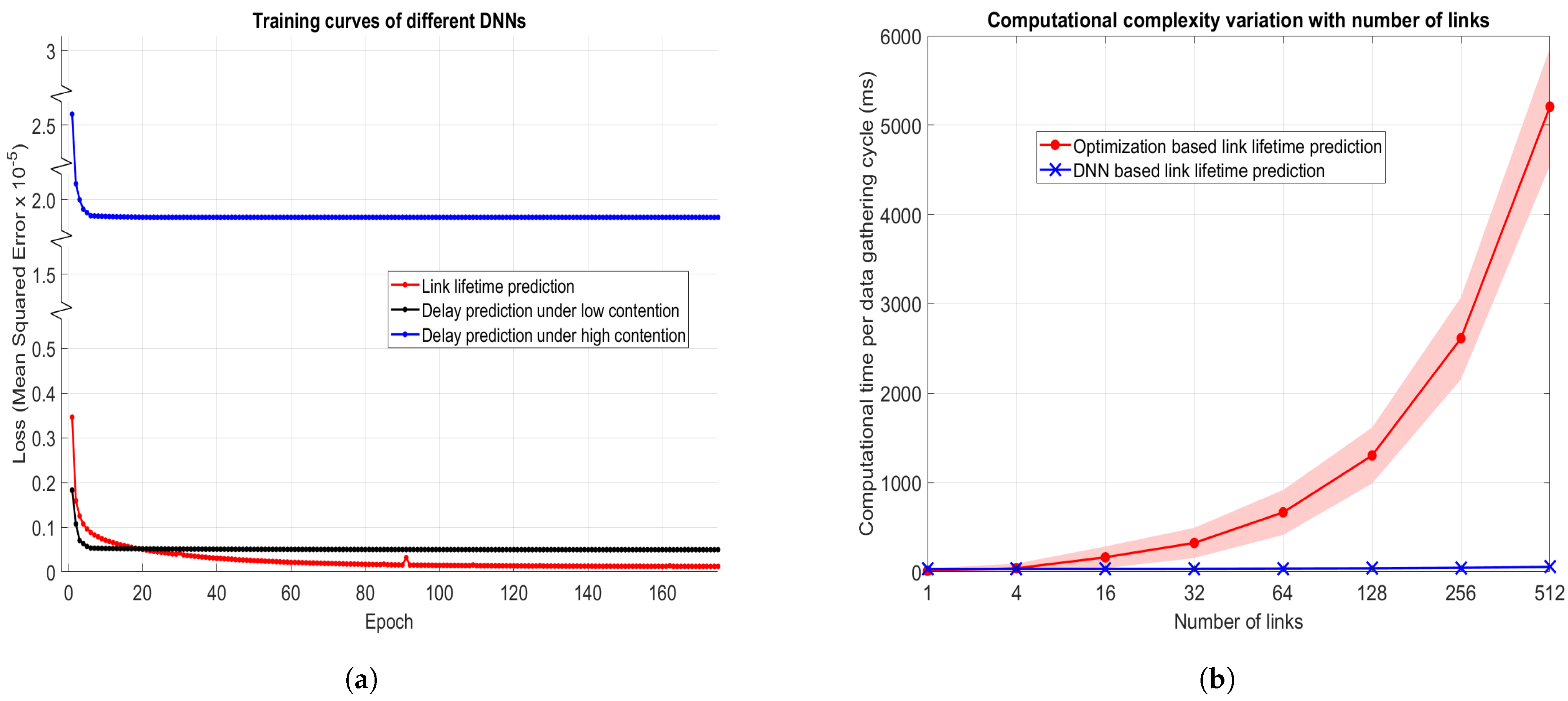
4.3. Performance of Wireless Link Lifetime Prediction and One-Hop Channel Delay Prediction Using DNNs

The training curves of DNNs for wireless link lifetime and one-hop channel delay predictions as well as the computational complexity comparison of wireless link lifetime prediction models are shown in Figure 15.
It is very clear in Figure 15a that all DNN models’ losses (Mean Squared Error) decayed exponentially with the number of epochs, such that all models were trained successfully. At the end of training, the wireless link lifetime prediction model’s loss was as low as 0.00000010, while that of one-hop channel delay prediction under low contention was as low as 0.00000049. Therefore, the wireless link lifetime prediction DNN was successfully trained to fit the actual wireless link lifetimes of vehicular networks, while the one-hop channel delay prediction model was successfully trained to fit the exact one-hop channel delay under low-contention scenarios. However, under high-contention scenarios, the loss in the one-hop channel delay prediction machine learning model at the end of training was as high as 0.000019, such that it was less suitable for one-hop delay prediction under high contention scenarios, as evident from Figure 15a, even though the training converged.
The test data set for wireless link lifetime prediction consisted of 673,712 samples using data collected entirely from a vehicular network. The DNN had a loss (mean squared error) of 0.00000011 and an RMSE of 0.000331 for the testing data set. As the wireless link lifetimes were normalized using a scale of 100 s, RMSE mapped to an error of only 33.1 ms between the predictions of the DNN and real wireless link lifetimes. Therefore, the DNN does a very good job of predicting wireless link lifetimes, as the 33.1 ms error was much smaller than the 100 s time frame.
The test data sets for one-hop channel delay prediction consisted of 700,000 samples, each for high-contention and low-contention scenarios. The low-contention scenario yielded a loss of 0.00000051 and an RMSE of 0.00071. The high-contention data set yielded a higher loss of 0.000019 and an RMSE of 0.00434. As the delay values were normalized on a scale of 100,000 μ s, the RMSE of the one-hop channel delay prediction DNN under low contention mapped to an error of 71 μ s, which was smaller than the 100,000 μ s time scale, while the 434 μ s error of the DNN predicting one-hop channel delay under high contention was significantly higher. This higher loss in a high-contention scenario occurs as a result of random contention delays caused by random backoff delays during the contention period. Thus, under high-contention scenarios, the one-hop channel delay prediction is more erroneous, so the routing algorithm should switch to distance mode.
Next, we analyzed the computational complexity of wireless link lifetime prediction for the DNN-based approach and the optimization-based approach. In this experiment, we varied the total number of wireless links and calculated the average computational time per wireless link per data gathering cycle ( T c o m ) using Equation (38). We computed the average value over 600 data gathering cycles. However, for the reader’s better understanding, we have shown the 95 % confidence interval variation of the computational time in Figure 15b. Note that the computational time of the DNN-based approach includes the data pre-processing (computing 2nd–8th-order terms and normalization) time along with prediction time.
It is crystal clear, as is evident from Figure 15b, that the average computational time per data gathering cycle increased for both the DNN-based approach and the optimization-based approach with the increment in the number of links. However, the increment was very low for wireless link lifetime prediction using the DNN, while a directly proportional relationship between computational time and number of links was observed for the optimization-based approach. This is because we can observe that, when the number of links doubles, the computational time per data gathering cycle also doubles for the optimization-based approach. On the other hand, for the DNN-based approach, the increment in computational time with the number of links is much smaller compared to the optimization-based approach. For instance, the average computational time for the DNN-based approach increased from 33.85 ms to 55.93 ms when the number of wireless links increased from 1 to 512. The computational time for the optimization-based approach was lower than the proposed DNN approach only when the number of links was less than two, as is evident from Figure 15b. However, vehicular networks consist of a large number of vehicles and RSUs, so the number of links that have to be predicted within a given data gathering cycle is usually large. Therefore, in large networks, as the number of links is high, we can conclude that the optimization-based wireless link lifetime prediction approach fails as the average computational time per data gathering cycle extends to thousands of milliseconds; thus, it will not be able to predict wireless link lifetimes, ensuring the latency requirements of vehicular networks. On the other hand, for the proposed wireless link lifetime prediction using a DNN, the average computational time was 55.93 ms when the number of links was 512. Furthermore, even if the number of links was much higher than 512 (say, 2000), according to the gradient of the graph, we can expect the average computational time for wireless link lifetime prediction using DNN to be less than 100 ms, thus successfully satisfying latency requirements for vehicular communication. Therefore, as the DNN-based approach has only an RMSE of 0.000331 and much lower computational complexity compared to the optimization-based approach, DNN can be replaced with the computationally inefficient optimization-based approach for wireless link lifetime prediction.

4.4. Routing Performance Evaluation

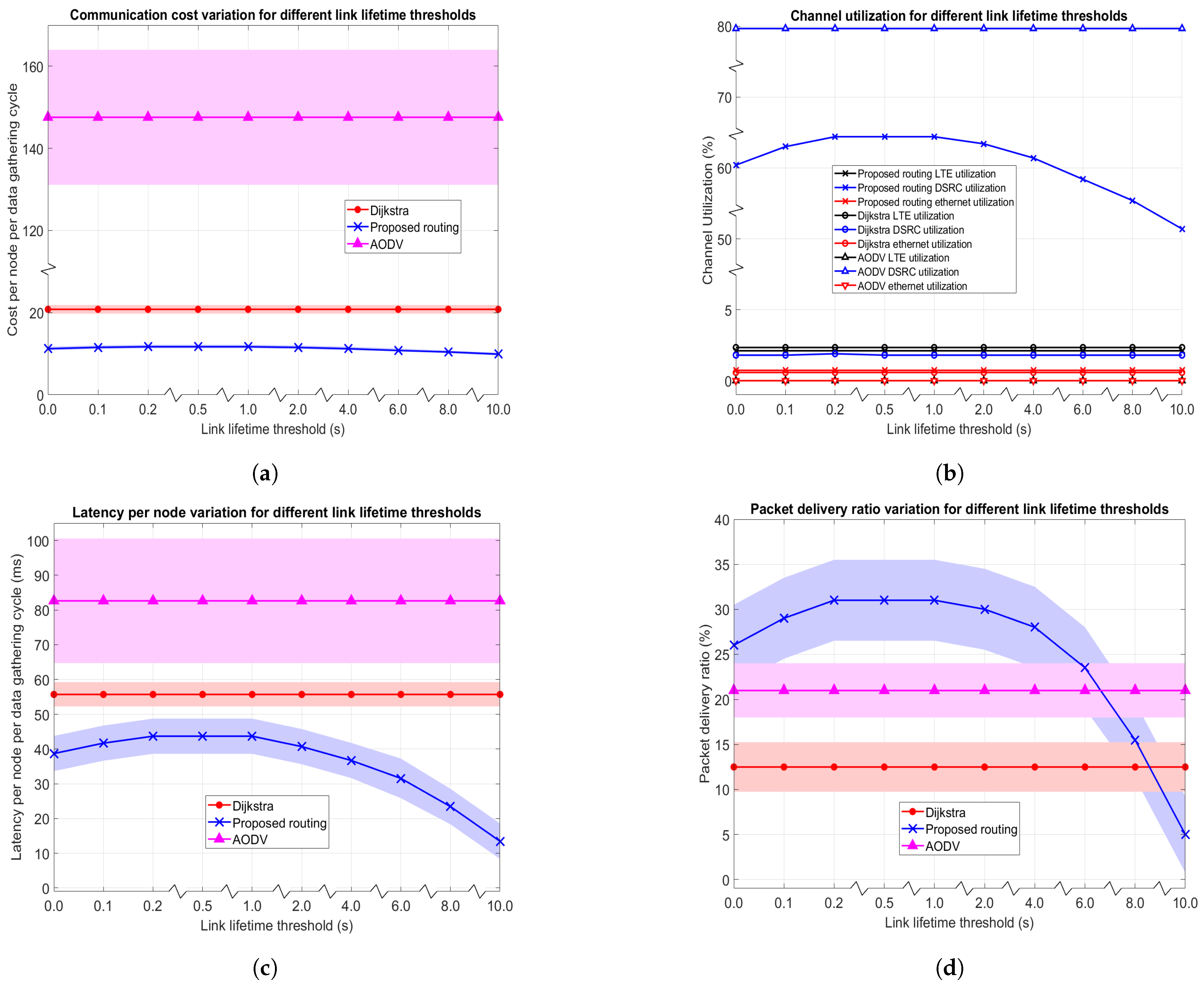
4.4.1. Impact of Link Lifetime Threshold

The maximum speed of the automobiles used in this experiment was set at 60 km/h, and data collection frequency (f), nominal optimization frequency ( f ) for the metadata collection, and routing frequency ( f ) were set to 1 Hz. Furthermore, 30 RSUs and 70 cars were present on the network in the aforementioned instance. The variable for the proposed routing framework was the link lifetime threshold ( T t h ), required for the algorithm in Figure 1, where we set the network contention threshold ( C t h ) to 0.50. No variable existed for the AODV or Dijkstra routing in this experiment. Variations in the T t h values were used to evaluate performance assessment metrics, and the findings are depicted in Figure 16. The 95 percent Confidence Intervals (CIs) are shown by colored regions in the graphs.
It is evident from Figure 16a that the proposed hybrid routing framework had the lowest average communication cost, compared to Dijkstra used for SDVN routing and AODV used for routing in VANET. The performance gap in communication cost between different routing methods was large, as the 95% CIs of each method were not overlapping and existed much apart from each other. The cost of the proposed routing was even less than Dijkstra, as Dijkstra involved proactive flow rule installation in each routing cycle for all entries in the flow table. On the other hand, the proposed routing uses an adaptive approach for route computation, flow rule update, and installation, which resulted in achieving the lowest communication cost, as evident from the results in Figure 16a. The communication cost of AODV was much higher than the other two routing methods for SDVN, as AODV involves the frequent exchange of packets through the network for route discovery on demand. On the other hand, the communication costs in routing methods for SDVN were much lower than for AODV, as routes are found using the metadata collected from the controller. The average communication cost did not vary with link lifetime thresholds from 0.2 s to 1.0 s, and the cost for the proposed routing was the highest (11.7) in that range. However, the communication cost for the proposed routing slowly increased in the link lifetime threshold range from 0 s to 0.20 s and began to slowly drop in the range from 1.0 s to 10.0 s, as evident from Figure 16a.
It is clear from Figure 16b that Ethernet and LTE utilization for AODV is zero, as those channels are not utilized in AODV. The DSRC utilization of the proposed method is always less than AODV and always higher than that of Dijkstra under any link lifetime threshold. Furthermore, the proposed method’s LTE utilization has always been lower and Ethernet utilization is always higher than those of routing using Dijkstra. The preceding fact is the reason for obtaining a lower communication cost in the proposed routing than Dijkstra, since Ethernet communication channels have a much lower cost per byte compared to cellular links. However, channel utilization does not reflect the number of packets routed or exchanged in the channel. Thus, the reason for the highest communication cost in AODV is due to the fact that it has the highest DSRC utilization of 80% and a very high number of packets exchanged for route discovery. For the proposed method, the DSRC utilization began to drop after the link lifetime threshold of 1 s, while it increased from 60% to 64% in the range of 0 s to 0.20 s.
When considering the latency variation in Figure 16c, the AODV routing for VANET had the highest latency, which was nearly two times the maximum value of latency for routing using the proposed routing. This high latency in AODV was due to the route discovery step at the time of routing, which increased the latency in routing. On the other hand, the proposed routing framework had nearly half the latency in AODV for link lifetime thresholds in the range 0 s to 2 s, while the latency approached zero at high link lifetime thresholds (e.g., 10 s), as evident from Figure 16c. However, this decrement in latency after the 1.0 s link lifetime threshold cannot be interpreted as a performance gain, as the packet delivery ratio also drops in the same manner for link lifetime thresholds greater than 1 s. Thus, for routing in SDVN architectures (Dijkstra and proposed routing), the latency is lower than AODV, as routes are computed by the controller using the metadata collected from the network. The latency of the proposed method is the lowest under any link lifetime threshold value, as the proposed method has the highest stable least delay mode, which selects low latency paths for packet routing under low contention scenarios. Thus, although the adaptive flow rule installation approach in the proposed method introduces some delay compared to the proactive approach, it was successfully compensated by the selection of low-delay routing paths by the proposed routing technique, resulting in the least latency out of the three routing approaches.
According to Figure 16d, it is very clear that the proposed routing framework had the highest PDR for link lifetime thresholds in the range of 0 s to 6 s. However, the average PDR dropped well below that of AODV by the link lifetime threshold of 8 s, and the average PDR dropped below both AODV and Dijkstra by the link lifetime threshold of 10 s. Furthermore, the PDR of AODV was much higher than routing in SDVN using Dijkstra, as evident from Figure 16d. The reason behind Dijkstra’s poor PDR compared to AODV is due to the fact that it computes routes using a shortest path algorithm that is unaware of the existence of the links. On the other hand, AODV discovers routes on demand, making sure that routing occurs only on existing links. Results on PDR given in Figure 16d show that a link lifetime threshold for the proposed routing must be carefully selected to maximize the packet delivery ratio. This shows that selecting either a very low or very high threshold can degrade the PDR of the proposed method.
Next, we analyzed the overall results of this experiment and decided on the optimum value of the link lifetime threshold for the rest of the experiments. It was clear from Figure 16a–d that communication cost, DSRC utilization, latency, and PDR of the proposed routing increased from link lifetime thresholds increasing from 0 s to 0.20 s, then remained at the highest value in the range of 0.2 s to 1.0 s, and then slowly degraded for link lifetimes greater than 1.0 s. Even though the highest values of communication cost, DSRC utilization, and latency existed at link lifetime thresholds of 0.20 s to 1.0 s, the highest PDR also occurred at the same specified range. We proposed this routing framework for SDVNs to increase the reliability of routing. When analyzing this result on link lifetime threshold, it is very clear that, if a link lifetime threshold lesser than 200 ms is set, those links that are added to the routes using the routing algorithm that have a link lifetime lesser than 200 ms will most probably not be available at routing time. That is the reason for obtaining a lower PDR in the range from 0.0 s to 0.2 s. Thus, the minimum experimental value for the link lifetime threshold can be inferred to be 200 ms. On the other hand, when a higher link lifetime threshold greater than 1.0 s is set for the proposed routing method, links that really exist at the routing time (for example, a link with a lifetime of 600 ms) will not be added to the routes using the hybrid routing algorithm due to the high link lifetime threshold. The preceding fact is the reason for obtaining a decreasing trend in PDR when the link lifetime threshold is increased beyond 1 s. Therefore, for the rest of this paper, unless otherwise specified, we set the link lifetime threshold at 0.2 s, since it is the minimum experimental link lifetime threshold value that achieves the highest PDR.

4.4.2. Impact of Routing Frequency

In this experiment, a similar urban transportation scenario with 40 automobiles and 20 RSUs in the simulation and a maximum vehicle speed set to 60 km/h were used. We set C t h = 0.5 and T t h = 0.2 , as experimentally found in Section 4.4.1. We set the data collection frequency (f), the nominal optimization frequency ( f ), and the routing frequency ( f ) equal to each other. Therefore, the variables in this experiment for all architectures were f, f , and f , which were synchronized together. The results obtained accordingly are shown in Figure 17.
The proposed link stability-based routing method had the least communication cost, compared to Dijkstra and AODV for any routing frequency, as evident from Figure 17a. The average communication costs of proposed routing and Dijkstra increase with increasing routing frequency. However, the gradient of cost increment in increasing order is the proposed routing and Dijkstra, as evident from Figure 17a. The gradient of cost increment with frequency is much lower in magnitude in Dijkstra and the proposed routing compared to the magnitude of the gradient of cost reduction in AODV with increment of frequency. The communication cost per data gathering cycle is much higher in AODV at lower frequencies. That is due to the fact that AODV is a routing protocol in VANET that sends packets for discovering routes during the entire routing cycle, which results in very high communication costs when the routing cycle period is long (routing frequency is low). On the other hand, for routing in SDVNs (Dijkstra and proposed routing), metadata are collected by the controller only once for the entire routing period, such that the communication cost is much lower than AODV. However, the average communication cost of AODV approaches routing in SDVNs when the routing frequency is higher. The average communication cost of Dijkstra is higher than proposed routing, as Dijkstra uses a proactive approach for flow rule installation, while the proposed method uses an adaptive approach that causes a lower communication cost due to the lesser number of FlowMod packets unicasted from controller to switches.
Next, we inspected the variation in channel utilization with respect to routing frequency. As evident from Figure 17b, all channel utilization for routing in SDVNs increases with frequency, while DSRC channel utilization for routing using AODV decreases with routing frequency. Ethernet and LTE channel utilization is always zero for AODV; thus, it does not vary with routing frequency. The DSRC utilization of AODV is closer to 100% at low routing frequencies, and it drops to 30.5% at 5 Hz. The reason for decreasing DSRC utilization with frequency in AODV is that, under low frequencies, it has enough time for route discovery and forwarding packets in the discovered routes. On the other hand, for the proposed routing method, the DSRC utilization was as low as 1.2% at 0.02 routing frequency, and gradually increased to 78.6% at 5 Hz routing frequency. For routing using Dijkstra, the DSRC utilization was very low at low routing frequencies, and it gradually grew to 12.4% by 5 Hz routing frequency. The reason for growing DSRC utilization with routing frequency in routing methods for SDVN is that the percentage of time during which the data plane routing takes place increases when the routing cycle period decreases (routing frequency increases). Another important fact to note in the results given in Figure 17b is that the proposed routing method’s Ethernet utilization is higher while the LTE channel utilization is lower than those of Dijkstra for any routing frequency. The reason for the preceding observation is because the proposed routing method utilizes adaptive flow rule computation, updating, and communicating flow rules to the switches along with an optimization framework for metadata collection, such that it reduces LTE utilization, which has a higher communication cost, while increasing Ethernet communication, since Ethernet communication has a relatively lower cost.
As is evident from Figure 17c, the end-to-end latency of routing using Dijkstra slowly increases with the routing frequency, which has a similar gradient to the proposed routing. The reason for the latency increment with routing frequency in Dijkstra is due to more packets being delivered with the increment of routing frequency, as evident from Figure 17d, even though it is a shortest path algorithm that does not take delay into account for its routing decisions. For the proposed routing as well, an increasing trend in average latency can be observed with an increment in routing frequency. One of the reasons for observing an increasing trend with routing frequency for the proposed method is that it has control over delay in its algorithm. Specifically, if the network contention is less than the contention threshold, it switches to the mode with the highest stable least delay, and otherwise switches to the highest stable least distance mode. Thus, due to the selection of the least delay paths by the proposed routing, the latency of the proposed routing is always less than Dijkstra for any routing frequency. Note that routing frequency can be associated with network contention as follows. The network contention depends on other factors such as pending packet transmissions (how packet routing is scheduled) and network link entropy, as explained in the methodology section. Thus, with an increment in routing frequency, there can be an increment in pending transmissions, since pending transmissions from the previous routing cycle can exist in the present routing cycle when the routing frequency is high. Therefore, contention can increase with routing frequency. With high contention, the proposed routing method tends to select the highest stable least distance mode at higher frequencies. The other reason behind the increment in average latency for the proposed method is due to delivering more packets at higher frequencies, as is evident from Figure 17d. Thus, due to the combination of those two reasons, the latency of proposed routing increases with routing frequency. In contrast, for routing using AODV in VANET, latency tends to decrease with increments in routing frequency. When the routing frequency was as low as 0.02 Hz, the average latency of AODV could be as high as 1097 ms. This high latency is due to the fact that routes are discovered in AODV on demand, which costs AODV in terms of latency. Thus, when routes are discovered and then packets are routed in AODV, the latency is higher than routing in SDVN. However, the latency of AODV approaches that of the proposed method at higher frequencies, as the latency gap between the proposed routing and AODV reduces with the increment of routing frequency, as evident from Figure 17c.
When analyzing the results for packet delivery ratio variation with routing frequency in Figure 17d, it is clear that both the proposed routing and Dijkstra’s PDR increase with increasing routing frequency. This is because, for both the proposed method and Dijkstra, the routes are not computed at the time of routing (they are pre-computed by the controller using the collected metadata), and the increment in routing frequency enhances the PDR of those routing techniques. In contrast, for AODV, the increment in routing frequency degrades its PDR since, at high frequencies, there is less time for discovering routes in AODV. Furthermore, at lower frequencies, the routing reliability of the proposed method approaches that of AODV, as evident from overlapping 95% confidence intervals and a lower gap between the PDR of the proposed method and AODV (shown in Figure 17d). Furthermore, the performance gap for reliability between AODV and Dijkstra decreases with increasing routing frequency, as, with increasing routing frequency, the PDR of AODV degrades, while that of routing using Dijkstra improves. On the other hand, the PDR gap between the proposed routing and AODV widens, as the routing frequency increment enhances the proposed routing and deteriorates AODV.
Overall, as evident from Figure 17, all three of cost, channel utilization, and latency increase with routing frequency for the proposed routing method, which can be considered a disadvantage at high routing frequencies. However, the previous disadvantage can be traded off with the gain in PDR for the proposed method at high frequencies.

4.4.3. Impact of Network Size

It was discovered in Section 4.4.2 that, at 0.5 Hz, there was moderate cost, utilization, latency, and PDR for the suggested routing approach; thus, we set f, f , and f to 0.5 Hz in this experiment. We set C t h = 0.5 and T t h = 0.2 , as experimentally found in Section 4.4.1. We modeled an urban mobility scenario with a maximum vehicle speed of 60 kph. The ratio of RSUs to vehicular nodes was kept constant at 1:3. The total number of nodes in the vehicular network, which could range from 4 to 256, was the variable in this experiment for all routing strategies. Figure 18 displays the results of evaluating the performance of routing techniques by adjusting the total number of nodes.
As seen from Figure 18a, AODV has the highest average communication cost except in very small networks (network size less than or equal to eight). On the other hand, the proposed routing method has the lowest communication cost out of all routing methods for any network size, except for a network with four nodes. As evident from Figure 18, for the network size of four, there is zero DSRC utilization, zero latency, and zero packet delivery ratio, which is exactly the reason for observing least cost for all routing methods. Thus, a network size of four is a total isolated network in which none of the nodes are connected to each other (zero network link entropy). Note that the costs of routing methods for SDVN (proposed routing and Dijkstra) are non-zero even in a total-isolated network, since the controller collects metadata using cellular and Ethernet links. The communication cost for all routing methods increases with the increment of network size, having a gradient of increment in ascending order as the proposed routing, Dijkstra, and AODV. For large networks (e.g., a network size of 256), the proposed method is very effective in reducing average routing communication costs, as it had a gap of 33.5 with Dijkstra and a gap of 610.7 compared with AODV.
It is very clear from Figure 18b that all channel utilizations, except LTE and Ethernet utilization of AODV, increase with the increase in the of number of nodes in the network. The DSRC utilization of routing methods is zero at a network size of four, since no packets are delivered in a totally isolated network. Another important fact to note is that the proposed method’s Ethernet utilization is higher while the LTE utilization is lower than those of routing using Dijkstra, except at a network size of four, in which those utilizations overlap. Furthermore, the gap between LTE utilization and Ethernet utilization between the proposed routing and Dijkstra increases with the increment in network size. The increasing order of DSRC utilization for any network size is Dijkstra, then proposed routing, and then AODV. Another important fact to note from the channel utilization results in Figure 18b is that the DSRC utilization gap between the proposed method and AODV reduces with increments in network size. The reason for obtaining the highest DSRC utilization for AODV is due to the fact that it utilizes DSRC for both route discovery and packet routing. On the other hand, both Dijkstra and the proposed routing use DSRC for one-hop broadcast for metadata collection and then for packet routing in a given routing cycle, which yields lower utilization than AODV. The lowest DSRC utilization for any network size is observed for routing using Dijkstra, which can be explained due to its lower PDR, as evident from Figure 18d.
When observing the results on the latency variation of routing methods under different network sizes, as shown in Figure 18c, it is clear that the average end-to-end latency for all routing methods increases with the increment of network size. The gradient of increment in latency in the increasing order is the proposed routing, Dijkstra, and AODV. Note that, when the average latency of Dijkstra grew from 9.88 ms to 136.11 ms, the average latency of the proposed routing only grew from 6.64 ms to 106.24 ms when the network size increased from 8 to 256. The proposed method yields low latency due to its mode, which is the highest stable and least delayed mode under low-contention scenarios. The preceding mode results in a significant latency reduction compared to the Dijkstra shortest path algorithm when the network size is large, as evident from Figure 18c. Furthermore, at node size four, the latency of all routing techniques is zero, as no packets are delivered on average by any of the routing methods. Thus, the latency gap between the routing techniques at lower network sizes is low, and the performance gap widens with the increment in network size, as evident from Figure 18c. The reason for the increment in latency with network size is that the average number of hops per route increases with the increment in network size. Thus, when packets are forwarded through a large number of hops, the average latency for routing increases. Furthermore, the low latency of Dijkstra compared to AODV does not make it superior to AODV because Dijkstra has the least PDR, as evident from Figure 18d. On the other hand, the proposed routing method achieves the lowest average latency values while at the same time achieving the highest PDR, which is a remarkable achievement.
The results for PDR variation with vehicular network size given in Figure 18d give an insight into the reliability of the routing techniques assessed in this research. As is evident from Figure 18d, the PDR of all routing techniques improves with increasing network size. For smaller network sizes (for example, network sizes of 4 and 8), the PDR gap between the routing techniques is very low, as evident from the overlapping data points and 95% CIs in Figure 18d. In the case of a network of size four, the vehicular network was a network consisting of all nodes being isolated such that the PDR of all routing methods was zero. On the other hand, with the increment in network size, the PDR gap between the routing techniques tends to widen. The increasing order of average PDR for large networks is Dijkstra, AODV, and the proposed routing. However, note that the reliability performance gap between the proposed routing and AODV is slightly wider compared to the PDR gap between AODV and Dijkstra for large networks. Furthermore, for large networks, the lower 95% CI of PDR for proposed routing lies above the upper 95% CI of PDR for AODV, such that the PDR of proposed routing is defensibly better than AODV for large networks under the settings for this experiment.
Overall, all communication cost, channel utilization, and latency tend to increase with the increment in network size for the proposed routing, as evident from Figure 18. However, the important thing to note is that average PDR also grows with network size, which compensates for the extra communication costs, channel utilization, and latency that occur in large networks.

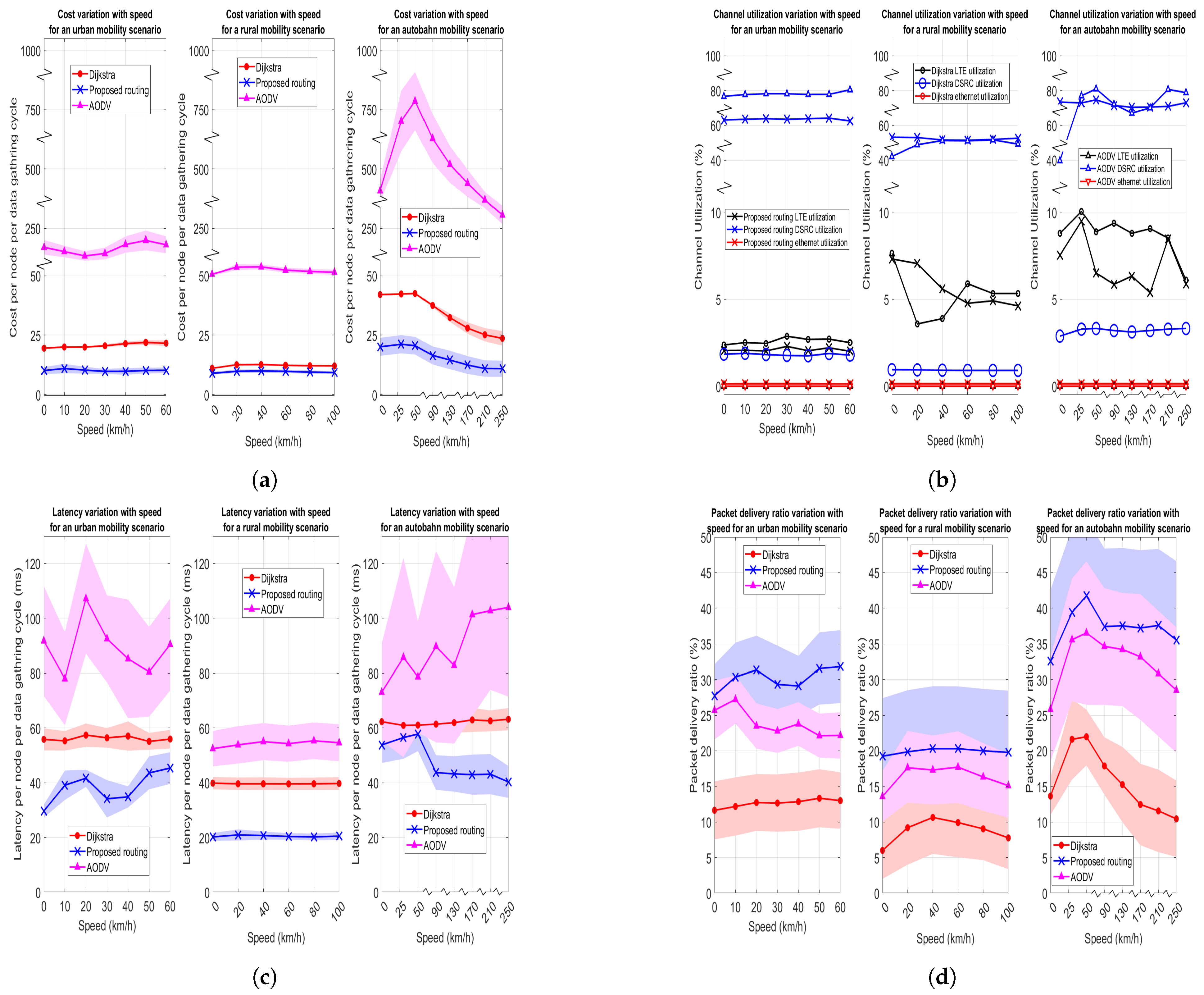
4.4.4. Impact of Vehicular Mobility

In this experiment, there were 72 vehicles and 24 RSUs in the vehicular network, and the data collection (f), nominal optimization ( f ), and routing frequencies ( f ) were all set to 0.5 Hz. According to Section 4.4.2, the proposed method produced moderate cost, channel utilization, latency, and PDR. The experiment’s dependent variable was the maximum speed at which cars were permitted to travel in each of the three mobility scenarios—autobahn, urban, and rural. The findings are shown in Figure 19. The suggested routing technique, Dijkstra, and AODV were assessed for each of the mobility situations by adjusting the maximum permitted speed of the vehicles.
When observing the cost variation with mobility, it is evident from Figure 19a that, under any mobility scenario or under any allowable maximum speed, the increasing order of average communication cost is always in the order of proposed routing, Dijkstra, and AODV. Thus, under any mobility scenario, the proposed routing yields the lowest average communication cost. However, the communication cost gap between the proposed routing and other methods is much lower for the rural mobility scenario. For the autobahn mobility scenario, an increasing trend in communication cost for all routing techniques can be observed for speeds in the range 0–50 km/h, and then a clear decreasing trend can be observed for high speeds in the range 50–250 km/h. Similarly, for the rural mobility scenario, an increasing trend in communication cost can be observed for speeds in the range 0–40 km/h, and then a decreasing trend can be observed for speeds in the range 40–100 km/h for all the routing methods. However, for the urban mobility scenario, the communication cost variation among routing methods differs. For the proposed routing in the urban mobility scenario, the cost increases from 0 to 10 km/h and then decreases slowly afterwards, while the cost of Dijkstra increases slowly with speed, whereas for AODV, a clear variation with speed cannot be observed. Furthermore, the cost for each of the methods under any speed in increasing order is rural, urban, and autobahn. The reason for the preceding order is the average network link entropy resulting from node density and the maximum transmission distance in each of the mobility scenarios. For example, the rural mobility scenario has the lowest node density (3000 m × 3000 m/96 nodes) and a moderate maximum transmission distance (41 dBm), resulting in the least average network link entropy and the least communication cost among mobility scenarios.
When considering the variation in channel utilization with mobility, the LTE and Ethernet channel utilization of AODV does not vary with mobility scenario or speed and always remains at zero, as evident from Figure 19b. The DSRC utilizations of the proposed method and Dijkstra almost do not vary with speed for a given mobility scenario. However, the increasing order of DSRC utilization for the proposed method and Dijkstra is rural, urban, and autobahn. The preceding order explains the reason for obtaining communication cost variation, also in the exact same order for those two routing approaches. However, the DSRC utilization of AODV tends to vary with speed in a given mobility scenario. Specifically, for the urban mobility scenario, the DSRC utilization of AODV tends to increase slightly with speed; for the rural mobility scenario, it tends to increase with speed except in the range 80–100 km/h; and for the autobahn mobility scenario, a clear variation cannot be observed. The DSRC utilization of the proposed routing was lower than that of AODV at all speeds for the urban and rural mobility scenarios, while it was higher and lower at different speeds in the autobahn mobility scenario. Another observation that can be seen from Figure 19b is that the LTE utilization of Dijkstra was always higher than that of the proposed routing at all speeds in urban and autobahn scenarios, while at higher speeds (and at zero speed in the rural mobility scenario), it occurred otherwise. The increasing order of LTE utilization of both the proposed routing and Dijkstra at all speeds among different mobility scenarios is urban, rural, and autobahn. However, increasing order of cost is not the preceding order, since communication cost in routing is affected mostly by DSRC utilization, whose variation is exactly the same as the communication cost variation.
The latency of routing using Dijkstra barely varies with speed in all mobility scenarios, as is evident from Figure 19c. Furthermore, under any mobility scenario, at any given speed, the increasing order of latency is the proposed routing, Dijkstra, and AODV. The latencies of each routing method are clearly separate from each other, as 95% CIs of latency of each routing technique do not overlap or intersect with each other for any speed in the urban and rural mobility scenarios. However, in the autobahn mobility scenario at lower speeds, 95% CIs of latency of routing techniques intersect, such that the latency gap is lower. Furthermore, for all routing techniques, the increasing order of latency among different mobility scenarios is rural, urban, and autobahn. For the rural mobility scenario, the latency of the proposed method is almost constant with speed, while the latency of AODV slightly increases with speed. In contrast, for the urban mobility scenario, a clear variation with speed cannot be observed for both the proposed routing method and AODV, as the latency tends to increase and decrease alternately with the increment of speed. However, for the autobahn mobility scenario, an increasing trend in latency for speeds in the range 0–50 km/h and a decreasing trend in latency for speeds greater than 50 km/h for the proposed routing can be observed, while an increasing trend in latency with speed for AODV can be observed.
The increasing order of packet delivery ratio among all speeds for a given routing technique among different mobility scenarios is rural, urban, and autobahn, as evident from Figure 19d. The reason for the preceding order of packet delivery ratios is that, when the average number of neighbors in the network increases, the PDR also increases. Thus, the average number of neighbors in the network should be in increasing order of rural, urban, and autobahn. Furthermore, for a given mobility scenario at any speed, the increasing order of packet delivery ratio is Dijkstra, AODV, and proposed routing. Thus, the proposed routing technique yields the best PDR at any speed in any mobility scenario. However, the PDR gap between the proposed method and AODV is low, as evident from the intersecting 95% CIs of PDRs of those techniques in Figure 19d. Note that, for all mobility scenarios, the PDRs of all routing techniques except AODV in the urban mobility scenario increase from 0 to 50 km/h and then deteriorate when the speed is increased beyond 50 km/h. Thus, moderate speeds seem to have enhanced packet delivery ratios, while very low and high speeds have poor packet delivery ratios for the proposed routing framework and routing using Dijkstra.
Overall, all four of the cost, channel utilization, latency, and PDR of each routing technique at all speeds among different mobility scenarios in increasing order are rural, urban, and autobahn. The underlying reasons for the above observations related to mobility are discussed in the discussion section.

5. Discussion

For the SDVN architecture, we proposed a novel routing technique. We used the prospect of machine learning to estimate the wireless link lifetimes and channel delay at each hop using the metadata collected at the controller, where the mode of routing was decided by inspecting the knowledge generated as normalized network contention. The hybrid routing algorithm is a novel algorithm which has two modes: the highest stable least delay mode and the highest stable least distance mode, in which the mode was decided by using computed normalized network contention. Furthermore, if multiple links exist between two given nodes, both wireless and wired, the proposed method will effectively choose the best link considering the link lifetime and link delay parameters. Furthermore, we proposed an adaptive approach for flow rule computation, update, and installation, to effectively reduce the communication cost. Thus, the proposed routing approach ensures that routing will only occur on stable links selected using the link lifetime matrix and delay matrix generated with the aid of machine learning, resulting in a higher PDR (reliability), a lower latency, and a lower cost than the other routing techniques compared in this research. We compared the proposed routing framework’s performance against Dijkstra, which is a shortest path algorithm for routing in SDVNs, and against AODV, which is used in VANET.
The amount of time between a packet being created at a source and it being delivered to its destination is known as latency. In other words, it is the longest air interface delay that may be tolerated in direct mode. When sending V2X messages from a UE supporting one V2X application to an RSU via another UE supporting a V2X application, vehicular communication may handle a maximum delay of 500 ms. Furthermore, a minimal 100 ms latency for human-assisted driving is permitted for the Basic Safety Message (BSM) broadcast and equivalent applications of the Collaborative Awareness Message for V2V safety [76]. However, BSM does involve only one-hop broadcasts, and the previous 500 ms maximum is defined for a two-hop scenario. Thus, end-to-end latency per hop should be compared with the standard to check whether latency violations occur. As per the results, the average latency of the proposed method in a network of 256 nodes was only 106.24 ms, which was for a multihop scenario. Thus, the multihop average latency of the proposed routing method lies well below the maximum 500 ms latency defined for a two-hop scenario for vehicular communication. Therefore, the proposed routing method is well suited to be employed in vehicular communication applications without violating latency constraints. The proposed routing technique reduces latency by selecting the highest stable least delay mode under low contention scenarios, which effectively selects stable and low delay paths for routing. Although the proposed adaptive flow rule computation, updating, and installation approach may introduce some latency compared to the proactive approach, it has been successfully nullified by the highest stable least delay mode in the proposed routing technique, which has caused it to yield the least latency among the routing techniques.
The maximum allowable packet loss rate at the application layer is referred to as reliability [88]. Based on transmission length and use, the trustworthiness (reliability) of vehicular communication is specified. Reliability for human-aided driving is typically as low as 20% when using the cooperative awareness message for V2V safety and the Basic Safety Message (BSM) broadcast [76]. In multihop scenarios, the PDR can be poor in vehicular networks due to the presence of isolated nodes in the network. It was proven in the results section that the average PDR of the proposed routing framework can be as high as 43.6% in large vehicular networks, which is much higher than that of Dijkstra (25.2%) and considerably higher than routing in VANET, which uses AODV (32%). The proposed routing framework yields a higher PDR based on two facts. The first one is that only stable links exist in the computed routes, ensuring that the routes really exist at the time of routing. The second one is that, when there are multiple links between two given nodes in different communication channels, it examines the link lifetime of the two candidate links and selects the link with the highest lifetime (in the highest stable least distance mode) or examines the combined effect of link lifetime and link delay (in the highest stable least delay mode) and chooses the communication channel that will ultimately lead to higher reliability compared to other routing techniques.
Although there is no widely accepted standard value for the maximum tolerable communication cost for routing in SDVN, it is always better to use a routing approach that results in the least communication cost. The communication cost metric that we calculated depicts the average communication cost per node per routing cycle, which includes both control plane communication and data plane communication costs that occurred while forwarding packets from given sources to destinations. In all research experiments, the proposed routing technique yielded the lowest average communication cost under any link lifetime threshold, routing frequency, network size, or mobility scenario under any speed, compared to Dijkstra and AODV, which is a remarkable achievement. This result verifies the strength of the proposed adaptive flow rule computation, updating, and installation approach, which updates the switches with the latest flow rules only when the flow rules installed in the switches expire, which results in the least cost compared to proactive flow rule installation in Dijkstra and the distributed routing approach in AODV.
Optimization can be used to achieve different objectives in computer networks. In [89], ant colony optimization has been utilized for cooperative multiple task reallocation under target precedence constraints for unmanned aerial vehicular networks. Furthermore, swarm intelligence algorithms such as particle swarm optimization, artificial fish farm, etc. have been proposed to optimize tasks in vehicular networks [90]. Similar to these studies, we modeled wireless link lifetime prediction as a non-linear optimization problem. Wireless link lifetime prediction using deep learning was experimentally proven to be much more computationally efficient than the optimization-based approach, which has a constraint with fourth-order terms. Deep learning utilizes the power of batch predictions and large data set training to accurately predict link lifetimes with much lower computational complexity compared to optimization. Therefore, deep learning stands out as a scalable solution for wireless link lifetime prediction, as the latency of the optimization-based approach extends to the order of seconds, as proved by the results.
Both wireless link lifetime prediction and one-hop channel prediction tasks require high accuracy in order for the proposed routing framework to be effective. Deep learning has been proven to provide highly accurate regression when trained with large labeled data sets [91]. Another reason for the choice of deep learning for prediction tasks is that deep learning is scalable and can handle large volumes of data at once, using its capability for batch predictions [92]. The input vector sizes of deep learning models for wireless link lifetime prediction and one-hop channel delay prediction are 104 and 30, respectively. However, predictions are made for the whole network by using batch predictions rather than predicting for individual links or individual nodes one after another. Thus, the total maximum input data size per network becomes 52 N 2 and 60N for wireless link lifetime prediction and one-hop channel delay prediction, respectively, which can result in a large volume of input data when the network size grows. Deep learning models are better suited for such large data predictions than other traditional supervised machine learning approaches. We trained the DNNs using large labeled data sets of 3,368,564, and 3,350,000 samples for wireless link lifetime prediction and one-hop channel delay prediction. Furthermore, it has been noted that deep learning models are well-suited for non-linear regression tasks because they can learn non-linear relationships between the input and output variables [93]. The wireless link lifetime prediction problem is an optimization task whose solution can be approximated by a polynomial combination of 8th-order terms of differential position, velocity, acceleration, etc. The relationship between the input variables and the output for the one-hop channel delay prediction is unknown. Therefore, to learn complex, unknown relationships between inputs and outputs, deep learning is well suited. Finally, deep learning models used for regression tasks have shown superior generalization performance over traditional machine learning approaches [94]. This is really important, as we train the machine learning models using a data set collected from some network scenarios that may not represent all states of the data. Thus, the regression models should have the capability to generalize, in order to predict unseen data with a low prediction error. Therefore, deep learning is an excellent choice to train the wireless link lifetime and one-hop channel delay using data collected from a network scenario, allowing them to generalize for unseen data. Wireless link lifetime prediction and one-hop channel delay prediction yielded very low RMSEs of only 0.000331 and 0.00071, respectively, proving to be highly accurate for the test data set. Such a low error in predictions must have been because we trained deep learning models using large labeled data sets for DNNs to learn complex relationships and generalize from input data, in order to accurately predict wireless link lifetimes and one-hop channel delays. Due to its low prediction error, it was not necessary to experiment on other machine learning techniques, as the main purpose of this research was to propose a novel routing approach for SDVNs, where link lifetime and delay predictions can be considered as sub-tasks in achieving the main purpose of routing. As the results on routing, based on DNN predictions, were proven to be superior over other routing techniques compared in this research, and, as discussed above, the existing literature proves that deep learning is superior for complex non-linear regression tasks when trained with large labeled data sets, there was no requirement to experiment with other machine learning techniques. Therefore, the accuracy of DNNs was highly satisfactory for making routing decisions.
The proposed routing technique is a link lifetime- and link delay-based routing framework that ensures that routing will only occur through stable links. For that purpose, as described in Section 3.4, the link lifetimes are inspected to check whether the link lifetime is greater than a specified threshold in order to determine the stability of the links. Metadata for computing routes is collected by the controller before scheduling routes. The links should be stable (exist) at least until the packet is delivered to the destination. Otherwise, if a very low link lifetime threshold such as 0.0 is set, links with a very low lifetime (say, 20 ms) will most probably not be available at the time of routing. On the other hand, if a very high link lifetime threshold is set, links that have a moderate link lifetime (say, 1 s) and really exist at the time of routing will not be added to the routes by the algorithm due to the high threshold. Thus, the optimum value should be selected experimentally. In Section 4.4.1, we experimentally found out that the optimum link lifetime threshold value was 200 ms, since link lifetime thresholds from 200 ms to 1000 ms gave the highest packet delivery ratio under the experimental settings.
In Section 4.4.2, results showed that the average communication cost, all-channel utilization, latency, and PDR of the proposed routing method and Dijkstra tend to increase with the increment of the routing frequency, while those of AODV degrade with the routing frequency. One of the reasons for the preceding observation is that both Dijkstra and proposed routing are used in SDVN, where the routes are computed by the centralized controller, which collects metadata from the vehicular network to compute the routes and control routing accordingly. However, in AODV, routes are computed on demand at the time of routing, such that, when it has little time for routing, i.e., when the routing frequency increases, its performance degrades. The other reason we can think of as the reason for incrementing PDR, etc., with routing frequency for the proposed routing is that we can expect the average network contention to increase with the increment of routing frequency, such that the proposed routing will switch more towards the most stable shortest path selection mode, which can increase latency, cost, and PDR, similar to the increment of the same in a shortest path algorithm such as Dijkstra with routing frequency.
In Section 4.4.3, we observed that the communication cost, channel utilization, latency, and PDR of all routing techniques increase with network size. The reason for that increment is the increment in average network link entropy and node density with network size, as the nodes are placed in a fixed-size map. However, the communication cost in an isolated network is non-zero for proposed routing and Dijkstra, as they collect metadata for computing routes at the controller. However, the latency, DSRC utilization, and PDR are zero for all routing techniques in an isolated network (network size of four), since that network must have zero average network link entropy (all nodes are isolated). With the increment in average network link entropy when the network size increases, the average number of hops per route in the network for routing packets increases, which is the reason for the increment in average latency with network size. The communication cost, channel utilization, and latency of distributed routing, such as AODV, are much higher than those of the proposed routing method for large networks due to the amplification of route discovery steps with network size. Furthermore, the PDR of the proposed method is significantly higher than both AODV and Dijkstra for large networks, while both the communication cost and latency of the proposed method are significantly lower than other routing techniques. Thus, for large networks, the proposed routing method yields superior performance to both AODV and Dijkstra.
In Section 4.4.4, we observed that the increasing order of communication cost, channel utilization, latency, and PDR for all routing techniques is rural, followed by urban, and then autobahn. The reason for the preceding order is that the average network link entropy varies in the same order due to the effect of both node density and maximum transmission power in each mobility scenario. When the average link entropy increases, the average number of neighbors for a given node also increases. Thus, the increasing order of average neighbors per given node is rural, urban, and autobahn, as explained by their corresponding node density and maximum transmission power values. Furthermore, it was observed that a given parameter for a given routing technique (e.g., latency of the proposed method) may have an increasing or decreasing trend, or no clear variation, with speed among different mobility scenarios. The reason for this could be that when changing the maximum allowable speed for a given mobility scenario, the underlying mobility pattern can be changed among different speeds for the same mobility scenario. However, it was evident that, when the speed increases beyond 50 km/h (e.g., 50–250 km/h in the autobahn scenario), the cost, latency, and packet delivery ratio decrease for the proposed routing, as the average link lifetime of the network tends to decrease with the increment in vehicular speeds. Even though the average link lifetime decreased in the range 0–50 km/h, the effect of the average network link entropy increment must have been more effective than the average link lifetime drop in that low speed range (0–50 km/h), which caused all communication cost, latency, and PDR to increase in that range for the proposed routing method.
Here, we statistically analyze the significance of the routing results obtained for the proposed framework compared to other approaches. Let us consider the three null hypotheses given below. Note that we compare the significance of a given parameter (cost, latency, and PDR) of the proposed method against the same parameter of another routing technique, which has overlapping or intersecting 95% CIs with the proposed method at some data points.
  • H1 —The communication cost of the proposed routing is higher than AODV;
  • H2—The end-to-end latency of the proposed routing is higher than Dijkstra;
  • H3—The PDR of the proposed routing is lower than AODV.
If the probability p (how likely it is that the data could have arisen by chance under the assumption that the null hypothesis is true [95]) is less than a significance level (a significance level of 0.05 is considered for this research), the alternative hypothesis can be accepted by rejecting the null hypothesis [96]. Let P H 1 , P H 2 , and P H 3 represent the p-value for Hypothesis H1, the p-value for Hypothesis H2, and the p-value for Hypothesis H3, respectively. As per the results, P H 1 < 0.05 except for the network size of 4 nodes, which had a P H 1 value of 1.00. Therefore, the alternative hypothesis of H1 (the cost of the proposed routing is lower than AODV) is statistically significant under any link lifetime threshold, any routing frequency, any mobility scenario, and for networks larger than four nodes. Furthermore, according to the results, P H 2 < 0.05 except for network sizes of 4 nodes, 8 nodes, 16 nodes, and 32 nodes, and for maximum speed values of 0 km/h, 30 km/h, and 50 km/h in the autobahn mobility scenario, with P H 2 values of 0.50, 0.37, 0.28, 0.11, 0.15, 0.22, and 0.17, respectively. Thus, the null hypothesis H2 can be rejected against the alternative hypothesis of H2 (the end-to-end latency of the proposed method is lower than Dijkstra) for all instances except for smaller networks (less than or equal to 32) and at low speeds (0–50 km/h) in the autobahn mobility scenario. Finally, we analyze the statistical significance of the results on PDR. According to the results on routing, the value of P H 3 is less than 0.05, except in the instances given in Table 4.
Therefore, the null hypothesis (H3) can be rejected, and the alternative hypothesis (the PDR of the proposed method is higher than AODV) is statistically significant for link lifetime thresholds in the range [0.1, 2.0], routing frequencies greater than 0.10 Hz, network size greater than 64 nodes, and the urban mobility scenario at speeds 20 km/h, 50 km/h, and 60 km/h. However, even though hypothesis H3 cannot be rejected at the network instances given in Table 4, due to the associated values of statistical significance, note that the average value of the PDR of the proposed method is always higher than AODV, except at link lifetime thresholds greater than 6.0 and at a network size of 4 nodes.
The significance of this research is that the proposed routing framework results in higher reliability and lower latency on average for routing in SDVNs by selecting routes that have both high link lifetimes and a lower delay. Furthermore, the proposed routing framework effectively reduces the communication cost by using an adaptive flow rule computation, updating, and installation approach. The proposed method effectively reduces estimation errors in predicting link delays under high contention scenarios by switching to the highest stable least distance mode. As routing is the basis for information dissemination in vehicular networks, the proposed routing method is capable of routing packets without violating latency constraints while at the same time achieving reliability benchmarks in vehicular communication. However, in order to achieve such superior performance over other existing routing approaches, an optimum value for the link lifetime threshold (200 ms) was required to be determined.

6. Conclusions and Future Research

This paper presents a routing framework for software-defined vehicular networks. The proposed framework generates link lifetime and link delay matrices with the aid of machine learning and selects its operation mode using the computed average normalized network contention parameter. Wireless link lifetime estimation using a DNN resulted in a much lower computational time compared to the optimization-based approach for large networks, thus enabling the proposed routing technique to estimate wireless link lifetimes while satisfying latency requirements in vehicular networks. Both DNNs predicting wireless link lifetime and one-hop channel delay proved to be accurate, having RMSE values of only 0.000331 and 0.00071, respectively. The results related to routing performance evaluation showed that, once the optimum link lifetime threshold (200 ms) is selected, the proposed routing technique for SDVN yields the highest packet delivery ratio, the lowest latency, moderate channel utilization, and the least cost, on average, compared to routing using AODV and Dijkstra. Results further proved that the performance of the proposed technique improved with increments in routing frequency and network size, and at moderate speeds (0–50 km/h). Thus, it can be concluded that the proposed routing technique improves routing in SDVNs.
Furthermore, the results of this study prove that machine learning is more suitable for wireless link lifetime prediction than a computationally less efficient optimization-based approach. As this is the first study to scrutinize machine learning for exact one-hop channel delay prediction, which resulted in only a RMSE of 0.00071 under low contention scenarios, deep learning can be recommended for one-hop channel delay prediction given that the network normalized contention value is lower than 0.5. Based on the results, in order to deploy the proposed routing framework in a SDVN, an optimum link lifetime threshold set in the range of 200 ms to 1000 ms is recommended to obtain the best performance from the proposed routing framework, as setting a link lifetime threshold too high or too low causes relatively poor packet delivery ratios. As the average latency values resulted from the proposed routing lie much below the maximum latency allowed for vehicular communication, as discussed in Section 5, the proposed routing framework can be recommended to be used in an SDVN without any hesitation. Statistical analysis further proved the significance and superiority of the proposed routing framework compared to AODV and Dijkstra, where the proposed routing technique always resulted in statistically significant results for link lifetime thresholds in the range of 100 ms to 2000 ms, network size greater than 64, and routing frequency greater than 0.10 under any mobility scenario except the PDR. Even though it was not statistically significant, the average value of PDR for the proposed method was always higher than other routing techniques under any mobility scenario.
This research fills a gap in the existing literature by estimating the link lifetimes and delay of the heterogeneous links, using machine learning along with a novel hybrid routing algorithm and an adaptive flow table update algorithm. The proposed framework can be utilized to achieve high reliability in routing while, at the same time, achieving lower communication costs and latency. The proposed routing framework can be applied practically at the industrial level, as it has been designed to be compatible with the existing OpenFlow protocol. Academicians can use the proposed routing framework for further research in SDVN applications by utilizing the theoretical framework presented to yield better application performance due to better routing. Furthermore, this research opens avenues for applying machine learning to improve the operations of SDVNs by experimentally proving that parameter computation using machine learning yields better performance than algorithmic approaches.
However, the proposed routing framework is applicable only in an SDVN paradigm where there is a logically centralized controller for collecting metadata from the network to compute link delay and link lifetime matrices using machine learning required for computing optimum routes using the proposed hybrid routing algorithm. Furthermore, the statistical significance of the results compared to existing routing approaches is lower under low routing frequencies, low network size, and very high and very low link lifetime thresholds.
In future work, one may develop the proposed routing algorithm as a machine learning model that is trained to compute routes once all the metadata collected from the vehicular network are provided to the model, such that the whole routing framework will be based on machine learning. Furthermore, the routing framework proposed in this research for SDVN can be extended to its extended paradigm, Knowledge-Defined Vehicular Network (KDVN), as the proposed routing approach uses data-driven routing decisions with the aid of machine learning. Future researchers can further extend the proposed routing framework to consider additional QoS parameters in addition to link delay and link lifetime, such as communication cost of the channels, network congestion, etc., to update the proposed routing algorithm considering those additional parameters. Not only that, future research can combine the proposed routing framework for a load balancing scenario by integrating it with a machine learning model for network traffic prediction. Furthermore, the proposed routing algorithm can be modified by a future researcher to compute paths that adhere to delay constraints by employing a delay threshold in hybrid routing algorithm, to provide delay-based quality of service-aware routing.

Author Contributions

Conceptualization—P.A.D.S.N.W. and S.G.; methodology—P.A.D.S.N.W. and S.G.; software—P.A.D.S.N.W.; validation—P.A.D.S.N.W.; formal analysis—P.A.D.S.N.W.; investigation—P.A.D.S.N.W.; resources—P.A.D.S.N.W.; data curation—P.A.D.S.N.W.; writing—original draft preparation—P.A.D.S.N.W.; writing—review and editing— S.G.; visualization—P.A.D.S.N.W.; supervision—S.G. All authors have read and agreed to the published version of the manuscript.

Funding

This research received no external funding.

Data Availability Statement

Data and code are available from the authors upon reasonable request after publication.

Acknowledgments

This research is part of a research project that principal and corresponding author Patikiri Arachchige Don Shehan Nilmantha Wijesekara is pursuing for a degree at the University of Ruhuna.

Conflicts of Interest

The authors declare no conflict of interest.

Appendix A. Metadata Collection for Routing Framework

The cost per byte of cellular links is usually 20 times that of DSRC links [87], so, if those links are always utilized, even for metadata collection for routing, the average communication cost will be high. Thus, for metadata collection for the proposed routing framework in SDVN architecture, we used the optimization framework that was proposed by us in our previous work for SDVNs [65], which optimally collects data by reducing total communication cost, delay, and overhead. The objective function of that optimization framework for status data collection is given in Equation (A1):
m i n i m i z e C C N i = 1 N N i z i + C C A i = 1 N B i x i C O i = 1 N ( x i m S i z m )
Note that, in Equation (A1), C C N ,   C C A , and C O are optimization coefficients, whereas x and z are the decision variables. For the ith node, if x i = 1 , it is a unicasting agent node; otherwise, if z i = 1 , it is a broadcasting node. N represents the total number of nodes, while N i represents the total number of nodes in the neighborhood of the ith node. Furthermore, B i is the combined communication cost of the ith agent node. The objective given in Equation (A1) should be achieved, subject to the constraints given in Equations (A2) and (A3):
x i + m S i x m > = 1 ; i S
In Equation (A2), S is the set of one-hop neighbors in the whole vehicular network. The constraint given in Equation (A2) specifies that there should be at least one agent in the neighborhood of a given node, including the node itself.
z i + x i = 1 ; i S
The constraint in Equation (A3) specifies that broadcasting nodes and agent nodes should be mutually exclusive. Thus, using the optimization framework given in Equations (A1)–(A3), we optimally collect metadata for computing parameters at the controller required for the proposed routing algorithm in the SDVN paradigm. Note that, in order to have a fair comparison with the Dijkstra shortest path routing algorithm used for routing in SDVN, we use the same optimization framework for metadata collection.

Appendix B. Sample Delay Calculations

We can first inspect the best-case one-hop average delay in a scenario where there is a minimum contention delay ( ρ W I = 0 ,   ρ W L = 0 ) and the average queue size is 1 ( R i ¯ = 1 ). Such a scenario is possible when routing is scheduled with a large time gap. In such a scenario, the average DSRC and Ethernet one-hop delay can be calculated as shown in Equations (A4) and (A5) by substituting in Equations (32) and (33), respectively:
D i W L , m i n ¯ = R i ¯ × ( t t r a n s , i + 4 t p r o p , i ¯ + 4 t p r o c , i + t r t s + t c t s + t a c k + D I F S + C W m i n T s l o t 8 ) = 1 × ( ( ( 204 × 8 b ) / 27 Mbps ) + 4 × ( 333 m / 3 × 10 8 ms 1 ) + 4 × 12 μ s + 20 × 8 b / 27 Mbps + ( 14 × 8 b / 27 ) Mbps + ( 14 × 8 b / 27 ) Mbps + 50 μ s + 15 × 20 8 μ s ) = 60.4 μ s + 4.44 μ s + 48 μ s + 5.92 μ s + 4.15 μ s + 4.15 μ s + 50 μ s + 37.5 μ s = 214.5 μ s
Note that, in Equations (A4) and (A5), the total encapsulated routing packet size is 204 bytes; the DSRC data rate is 27 Mbps; the maximum transmission distance is 333 m; the Ethernet data rate is 1000 Mbps; the processing delay is considered to be 12 μ s, which is usually between 10 and 16 μ s [97]; and the Ethernet link distance is 1000 m.
D i W I , m i n ¯ = R i ¯ × ( t t r a n s , i + t p r o p , i ¯ + t p r o c , i + I F G ) = 1 × ( ( ( 204 × 8 b ) / 1000 Mbps ) + ( 1000 m / ( 0.64 × 3 × 10 8 ms 1 ) ) + 12 μ s + 9.6 μ s ) = 1.632 μ s + 5.21 μ s + 12 μ s + 9.6 μ s = 28.4 μ s

References

  1. Hamdi, M.M.; Audah, L.; Rashid, S.A.; Mohammed, A.H.; Alani, S.; Mustafa, A.S. A review of applications, characteristics and challenges in vehicular ad hoc networks (VANETs). In Proceedings of the 2020 International Congress on Human-Computer Interaction, Optimization and Robotic Applications (HORA), Copenhagen, Denmark, 26 June–1 July 2020; pp. 1–7. [Google Scholar]
  2. Hoebeke, J.; Moerman, I.; Dhoedt, B.; Demeester, P. An overview of mobile ad hoc networks: Applications and challenges. J.-Commun. Netw. 2004, 3, 60–66. [Google Scholar]
  3. Chlamtac, I.; Conti, M.; Liu, J.J.N. Mobile ad hoc networking: Imperatives and challenges. Ad Hoc Netw. 2003, 1, 13–64. [Google Scholar] [CrossRef]
  4. Dahiya, A.; Chauhan, R.K. A comparative study of MANET and VANET environment. J. Comput. 2010, 2, 87–92. [Google Scholar]
  5. Martinez, F.J.; Fogue, M.; Coll, M.; Cano, J.C.; Calafate, C.T.; Manzoni, P. Assessing the impact of a realistic radio propagation model on VANET scenarios using real maps. In Proceedings of the 2010 Ninth IEEE International Symposium on Network Computing and Applications, Cambridge, MA, USA, 15–17 July 2010; IEEE: New York, NY, USA, 2010; pp. 132–139. [Google Scholar]
  6. Alani, S.; Zakaria, Z.; Hamdi, M.M. A study review on mobile ad-hoc network: Characteristics, applications, challenges and routing protocols classification. Int. J. Adv. Sci. Technol. 2019, 28, 394–405. [Google Scholar]
  7. Sou, S.I.; Tonguz, O.K. Enhancing VANET connectivity through roadside units on highways. IEEE Trans. Veh. Technol. 2011, 60, 3586–3602. [Google Scholar] [CrossRef]
  8. Soni, M.; Rajput, B.S.; Patel, T.; Parmar, N. Lightweight vehicle-to-infrastructure message verification method for VANET. In Data Science and Intelligent Applications; Springer: Berlin, Germany, 2021; pp. 451–456. [Google Scholar]
  9. Seneviratne, C.; Wijesekara, P.A.D.S.N.; Leung, H. Performance analysis of distributed estimation for data fusion using a statistical approach in smart grid noisy wireless sensor networks. Sensors 2020, 20, 567. [Google Scholar] [CrossRef] [PubMed] [Green Version]
  10. Lee, M.; Atkison, T. Vanet applications: Past, present, and future. Veh. Commun. 2021, 28, 100310. [Google Scholar] [CrossRef]
  11. Wijesekara, P.A.D.S.N.; Sudheera, K.L.K.; Sandamali, G.G.N.; Chong, P.H.J. Data Gathering Optimization in Hybrid Software Defined Vehicular Networks. In Proceedings of the 20th Academic Sessions, Matara, Sri Lanka, 7 June 2023; p. 59. [Google Scholar]
  12. Haji, S.H.; Zeebaree, S.R.; Saeed, R.H.; Ameen, S.Y.; Shukur, H.M.; Omar, N.; Sadeeq, M.A.; Ageed, Z.S.; Ibrahim, I.M.; Yasin, H.M. Comparison of software defined networking with traditional networking. Asian J. Res. Comput. Sci. 2021, 9, 1–18. [Google Scholar] [CrossRef]
  13. Mishra, S.; AlShehri, M.A.R. Software defined networking: Research issues, challenges and opportunities. Indian J. Sci. Technol. 2017, 10, 1–9. [Google Scholar] [CrossRef]
  14. Nunes, B.A.A.; Mendonca, M.; Nguyen, X.N.; Obraczka, K.; Turletti, T. A survey of software-defined networking: Past, present, and future of programmable networks. IEEE Commun. Surv. Tutor. 2014, 16, 1617–1634. [Google Scholar] [CrossRef] [Green Version]
  15. Fonseca, P.C.; Mota, E.S. A survey on fault management in software-defined networks. IEEE Commun. Surv. Tutor. 2017, 19, 2284–2321. [Google Scholar] [CrossRef]
  16. Nisar, K.; Jimson, E.R.; Hijazi, M.H.A.; Welch, I.; Hassan, R.; Aman, A.H.M.; Sodhro, A.H.; Pirbhulal, S.; Khan, S. A survey on the architecture, application, and security of software defined networking: Challenges and open issues. Internet Things 2020, 12, 100289. [Google Scholar] [CrossRef]
  17. Jagadeesan, N.A.; Krishnamachari, B. Software-defined networking paradigms in wireless networks: A survey. ACM Comput. Surv. (CSUR) 2014, 47, 1–11. [Google Scholar] [CrossRef]
  18. Ku, I.; Lu, Y.; Gerla, M.; Gomes, R.L.; Ongaro, F.; Cerqueira, E. Towards software-defined VANET: Architecture and services. In Proceedings of the 2014 13th Annual Mediterranean Ad Hoc Networking Workshop (MED-HOC-NET), Piran, Slovenia, 2–4 June 2014; IEEE: New York, NY, USA, 2014; pp. 103–110. [Google Scholar]
  19. Bhatia, J.; Modi, Y.; Tanwar, S.; Bhavsar, M. Software defined vehicular networks: A comprehensive review. Int. J. Commun. Syst. 2019, 32, e4005. [Google Scholar] [CrossRef]
  20. Zhu, M.; Cai, Z.P.; Xu, M.; Cao, J.N. Software-defined vehicular networks: Opportunities and challenges. In Energy Science and Applied Technology; CRC Press: Boca Raton, FL, USA, 2015; pp. 247–251. [Google Scholar]
  21. Wijesekara, P.A.D.S.N.; Gunawardena, S. A Review of Blockchain Technology in Knowledge-Defined Networking, Its Application, Benefits, and Challenges. Network 2023. submitted. [Google Scholar]
  22. Zhao, L.; Li, J.; Al-Dubai, A.; Zomaya, A.Y.; Min, G.; Hawbani, A. Routing schemes in software-defined vehicular networks: Design, open issues and challenges. IEEE Intell. Transp. Syst. Mag. 2020, 13, 217–226. [Google Scholar] [CrossRef] [Green Version]
  23. Quan, W.; Cheng, N.; Qin, M.; Zhang, H.; Chan, H.A.; Shen, X. Adaptive transmission control for software defined vehicular networks. IEEE Wirel. Commun. Lett. 2018, 8, 653–656. [Google Scholar] [CrossRef]
  24. Islam, M.M.; Khan, M.T.R.; Saad, M.M.; Kim, D. Software-defined vehicular network (SDVN): A survey on architecture and routing. J. Syst. Archit. 2021, 114, 101961. [Google Scholar] [CrossRef]
  25. Adbeb, T.; Wu, D.; Ibrar, M. Software-defined networking (SDN) based VANET architecture: Mitigation of traffic congestion. Int. J. Adv. Comput. Sci. Appl. 2020, 11, 1–9. [Google Scholar] [CrossRef] [Green Version]
  26. Liu, K.; Xu, X.; Chen, M.; Liu, B.; Wu, L.; Lee, V.C. A hierarchical architecture for the future internet of vehicles. IEEE Commun. Mag. 2019, 57, 41–47. [Google Scholar] [CrossRef]
  27. Toufga, S.; Abdellatif, S.; Assouane, H.T.; Owezarski, P.; Villemur, T. Towards dynamic controller placement in software defined vehicular networks. Sensors 2020, 20, 1701. [Google Scholar] [CrossRef] [Green Version]
  28. Hinds, A.; Ngulube, M.; Zhu, S.; Al-Aqrabi, H. A review of routing protocols for mobile ad-hoc networks (manet). Int. J. Inf. Educ. Technol. 2013, 3, 1. [Google Scholar] [CrossRef] [Green Version]
  29. Shelly, S.; Babu, A.V. Link reliability based greedy perimeter stateless routing for vehicular ad hoc networks. Int. J. Veh. Technol. 2015, 2015, 1–16. [Google Scholar] [CrossRef] [Green Version]
  30. Pathak, C.; Shrivastava, A.; Jain, A. Ad-hoc on demand distance vector routing protocol using Dijkastra’s algorithm (AODV-D) for high throughput in VANET (Vehicular Ad-hoc Network). In Proceedings of the 2016 11th International Conference on Industrial and Information Systems (ICIIS), Roorkee, India, 3–4 December 2016; IEEE: New York, NY, USA, 2016; pp. 355–359. [Google Scholar]
  31. Dafalla, M.E.M.; Mokhtar, R.A.; Saeed, R.A.; Alhumyani, H.; Abdel-Khalek, S.; Khayyat, M. An optimized link state routing protocol for real-time application over Vehicular Ad-hoc Network. Alex. Eng. J. 2022, 61, 4541–4556. [Google Scholar] [CrossRef]
  32. Hamid, B.; El Mokhtar, E.N. Performance analysis of the Vehicular Ad hoc Networks (VANET) routing protocols AODV, DSDV and OLSR. In Proceedings of the 2015 5th International Conference on Information & Communication Technology and Accessibility (ICTA), Marrakesh, Morocco, 21–23 December 2015; IEEE: New York, NY, USA, 2015; pp. 1–6. [Google Scholar]
  33. Xie, J.; Yu, F.R.; Huang, T.; Xie, R.; Liu, J.; Wang, C.; Liu, Y. A survey of machine learning techniques applied to software defined networking (SDN): Research issues and challenges. IEEE Commun. Surv. Tutor. 2018, 21, 393–430. [Google Scholar] [CrossRef]
  34. Jiang, J.R.; Huang, H.W.; Liao, J.H.; Chen, S.Y. Extending Dijkstra’s shortest path algorithm for software defined networking. In Proceedings of the 16th Asia-Pacific Network Operations and Management Symposium, Hsinchu, Taiwan, 17–19 September 2014; IEEE: New York, NY, USA, 2014; pp. 1–4. [Google Scholar]
  35. Yanjun, L.; Xiaobo, L.; Osamu, Y. Traffic engineering framework with machine learning based meta-layer in software-defined networks. In Proceedings of the 2014 4th IEEE International Conference on Network Infrastructure and Digital Content, Beijing, China, 19–21 September 2014; IEEE: New York, NY, USA, 2014; pp. 121–125. [Google Scholar]
  36. Wang, J.; Miao, Y.; Zhou, P.; Hossain, M.S.; Rahman, S.M.M. A software defined network routing in wireless multihop network. J. Netw. Comput. Appl. 2017, 85, 76–83. [Google Scholar] [CrossRef]
  37. Azzouni, A.; Boutaba, R.; Pujolle, G. NeuRoute: Predictive dynamic routing for software-defined networks. In Proceedings of the 2017 13th International Conference on Network and Service Management (CNSM), Tokyo, Japan, 26–30 November 2017; IEEE: New York, NY, USA, 2017; pp. 1–6. [Google Scholar]
  38. Sendra, S.; Rego, A.; Lloret, J.; Jimenez, J.M.; Romero, O. Including artificial intelligence in a routing protocol using software defined networks. In Proceedings of the 2017 IEEE International Conference on Communications Workshops (ICC Workshops), Paris, France, 21–25 May 2017; IEEE: New York, NY, USA, 2017; pp. 670–674. [Google Scholar]
  39. Lin, S.C.; Akyildiz, I.F.; Wang, P.; Luo, M. QoS-aware adaptive routing in multi-layer hierarchical software defined networks: A reinforcement learning approach. In Proceedings of the 2016 IEEE International Conference on Services Computing (SCC), San Francisco, CA, USA, 27 June–2 July 2016; IEEE: New York, NY, USA, 2016; pp. 25–33. [Google Scholar]
  40. Alvizu, R.; Troia, S.; Maier, G.; Pattavina, A. Matheuristic with machine-learning-based prediction for software-defined mobile metro-core networks. J. Opt. Commun. Netw. 2017, 9, D19–D30. [Google Scholar] [CrossRef]
  41. Chen-Xiao, C.; Ya-Bin, X. Research on load balance method in SDN. Int. J. Grid Distrib. Comput. 2016, 9, 25–36. [Google Scholar] [CrossRef]
  42. Correia, S.; Boukerche, A.; Meneguette, R.I. An architecture for hierarchical software-defined vehicular networks. IEEE Commun. Mag. 2017, 55, 80–86. [Google Scholar] [CrossRef]
  43. He, Z.; Zhang, D.; Liang, J. Cost-efficient sensory data transmission in heterogeneous software-defined vehicular networks. IEEE Sensors J. 2016, 16, 7342–7354. [Google Scholar] [CrossRef]
  44. Dong, B.; Wu, W.; Yang, Z.; Li, J. Software defined networking based on-demand routing protocol in vehicle ad hoc networks. In Proceedings of the 2016 12th International Conference on Mobile Ad-Hoc and Sensor Networks (MSN), Hefei, China, 16–18 December 2016; IEEE: New York, NY, USA, 2016; pp. 207–213. [Google Scholar]
  45. Zhu, M.; Cai, Z.; Cao, J.; Xu, M. Efficient multiple-copy routing in software-defined vehicular networks. In Proceedings of the 2015 International Conference on Information and Communications Technologies (ICT 2015), Xi’an, China, 24–26 April 2015. [Google Scholar]
  46. Zhu, M.; Cao, J.; Pang, D.; He, Z.; Xu, M. SDN-based routing for efficient message propagation in VANET. In International Conference on Wireless Algorithms, Systems, and Applications, Qufu, China, 10–12 August 2015; Springer: Cham, Switzerland, 2015; pp. 788–797. [Google Scholar]
  47. Sudheera, K.L.K.; Ma, M.; Chong, P.H.J. Link stability based optimized routing framework for software defined vehicular networks. IEEE Trans. Veh. Technol. 2019, 68, 2934–2945. [Google Scholar] [CrossRef]
  48. Sudheera, K.K.; Ma, M.; Chong, P.H.J. Cooperative data routing & scheduling in software defined vehicular networks. In Proceedings of the 2018 IEEE Vehicular Networking Conference (VNC), 2018, Taipei, Taiwan, 5–7 December 2018; IEEE: New York, NY, USA, 2018; pp. 1–8. [Google Scholar]
  49. Sudheera, K.L.K.; Ma, M.; Chong, P.H.J. Real-time cooperative data routing and scheduling in software defined vehicular networks. Comput. Commun. 2022, 181, 203–214. [Google Scholar] [CrossRef]
  50. Liyanage, K.S.K.; Ma, M.; Chong, P.H.J. Connectivity aware tribrid routing framework for a generalized software defined vehicular network. Comput. Netw. 2019, 152, 167–177. [Google Scholar] [CrossRef]
  51. Ghafoor, H.; Koo, I. CR-SDVN: A cognitive routing protocol for software-defined vehicular networks. IEEE Sensors J. 2017, 18, 1761–1772. [Google Scholar] [CrossRef]
  52. Darabkh, K.A.; Alkhader, B.Z.; Ala’F, K.; Jubair, F.; Abdel-Majeed, M. ICDRP-F-SDVN: An innovative cluster-based dual-phase routing protocol using fog computing and software-defined vehicular network. Veh. Commun. 2022, 34, 100453. [Google Scholar] [CrossRef]
  53. Yuan, X.S.; Caballero, J.M.; Juanatas, R. A Highway Routing Algorithm Based on SDVN. In Proceedings of the 2022 14th International Conference on Communication Software and Networks (ICCSN), Chongqing, China, 10–12 June 2022; IEEE: New York, NY, USA, 2022; pp. 1–5. [Google Scholar]
  54. Awad, M.K.; Ahmed, M.H.H.; Almutairi, A.F.; Ahmad, I. Machine learning-based multipath routing for software defined networks. J. Netw. Syst. Manag. 2021, 29, 1–30. [Google Scholar] [CrossRef]
  55. Zhang, D.; Yu, F.R.; Yang, R. A machine learning approach for software-defined vehicular ad hoc networks with trust management. In Proceedings of the 2018 IEEE Global Communications Conference (GLOBECOM), Abu Dhabi, United Arab Emirate, 9–13 December 2018; IEEE: New York, NY, USA, 2018; pp. 1–6. [Google Scholar]
  56. Zhao, L.; Bi, Z.; Lin, M.; Hawbani, A.; Shi, J.; Guan, Y. An intelligent fuzzy-based routing scheme for software-defined vehicular networks. Comput. Netw. 2021, 187, 107837. [Google Scholar] [CrossRef]
  57. Wu, J.; Fang, M.; Li, X. Reinforcement learning based mobility adaptive routing for vehicular ad-hoc networks. Wirel. Pers. Commun. 2018, 101, 2143–2171. [Google Scholar] [CrossRef]
  58. Li, F.; Song, X.; Chen, H.; Li, X.; Wang, Y. Hierarchical routing for vehicular ad hoc networks via reinforcement learning. IEEE Trans. Veh. Technol. 2018, 68, 1852–1865. [Google Scholar] [CrossRef]
  59. Wijesekara, P.A.D.S.N. Deep 3D Dynamic Object Detection towards Successful and Safe Navigation for Full Autonomous Driving. Open Transp. J. 2022, 16, e187444782208191. [Google Scholar] [CrossRef]
  60. Herath, H.M.D.P.M.; Weraniyagoda, W.A.S.A.; Rajapaksha, R.T.M.; Wijesekara, P.A.D.S.N.; Sudheera, K.L.K.; Chong, P.H.J. Automatic Assessment of Aphasic Speech Sensed by Audio Sensors for Classification into Aphasia Severity Levels to Recommend Speech Therapies. Sensors 2022, 22, 6966. [Google Scholar] [CrossRef] [PubMed]
  61. Liyanage, K.S.K.; Ma, M.; Chong, P.H.J. Controller placement optimization in hierarchical distributed software defined vehicular networks. Comput. Netw. 2018, 135, 226–239. [Google Scholar] [CrossRef]
  62. Small, M. Complex networks from time series: Capturing dynamics. In Proceedings of the 2013 IEEE International Symposium on Circuits and Systems (ISCAS), Beijing, China, 19–23 May 2013; IEEE: New York, NY, USA, 2013; pp. 2509–2512. [Google Scholar]
  63. McKeown, N.; Anderson, T.; Balakrishnan, H.; Parulkar, G.; Peterson, L.; Rexford, J.; Shenker, S.; Turner, J. OpenFlow: Enabling innovation in campus networks. ACM SIGCOMM Comput. Commun. Rev. 2008, 38, 69–74. [Google Scholar] [CrossRef]
  64. Fernandez, M.P. Comparing openflow controller paradigms scalability: Reactive and proactive. In Proceedings of the 2013 IEEE 27th International Conference on Advanced Information Networking and Applications (AINA), Barcelona, Spain, 25–28 March 2013; IEEE: New York, NY, USA, 2013; pp. 1009–1016. [Google Scholar]
  65. Wijesekara, P.A.D.S.N.; Sudheera, K.L.K.; Sandamali, G.G.N.; Chong, P.H.J. An Optimization Framework for Data Collection in Software Defined Vehicular Networks. Sensors 2023, 23, 1600. [Google Scholar] [CrossRef]
  66. Wijesekara, P.A.D.S.N.; Wang, Y.K. A Mathematical Epidemiological Model (SEQIJRDS) to Recommend Public Health Interventions Related to COVID-19 in Sri Lanka. COVID 2022, 2, 793–826. [Google Scholar] [CrossRef]
  67. Riley, G.F.; Henderson, T.R. The ns-3 network simulator. In Modeling and Tools for Network Simulation; Springer: Berlin/Heidelberg, Germany, 2010; pp. 15–34. [Google Scholar]
  68. Wijesekara, P.A.D.S.N.; Sudheera, K.L.K.; Sandamali, G.G.N.; Chong, P.H.J. Machine Learning Based Link Stability Prediction for Routing in Software Defined Vehicular Networks. In Proceedings of the 20th Academic Sessions, Matara, Sri Lanka, 7 June 2023; p. 60. [Google Scholar]
  69. Wijesekara, P.A.D.S.N.; Gunawardena, S. A Comprehensive Survey on Knowledge-Defined Networking. Telecom 2023, submitted.
  70. Anand, R.; Aggarwal, D.; Kumar, V. A comparative analysis of optimization solvers. J. Stat. Manag. Syst. 2017, 20, 623–635. [Google Scholar] [CrossRef]
  71. Sharma, S.; Sharma, S.; Athaiya, A. Activation functions in neural networks. Towards Data Sci. 2017, 6, 310–316. [Google Scholar] [CrossRef]
  72. Wijesekara, P.A.D.S.N. An Accurate Mathematical Epidemiological Model (SEQIJRDS) to Recommend Public Health Interventions Related to COVID-19 in Sri Lanka. Prepr. Res. Sq. 2021. [Google Scholar] [CrossRef]
  73. Kandel, I.; Castelli, M. The effect of batch size on the generalizability of the convolutional neural networks on a histopathology dataset. ICT Express 2020, 6, 312–315. [Google Scholar] [CrossRef]
  74. Wijesekara, P.A.D.S.N. Deep 3D Dynamic Object Detection towards Successful and Safe Navigation for Full Autonomous Driving. Prepr. TechRxiv 2022. Available online: https://www.techrxiv.org/articles/preprint/Deep_3D_Dynamic_Object_Detection_towards_Successful_and_Safe_Navigation_for_Full_Autonomous_Driving/18517925 (accessed on 28 June 2022).
  75. Fogue, M.; Garrido, P.; Martinez, F.J.; Cano, J.C.; Calafate, C.T.; Manzoni, P. A realistic simulation framework for vehicular networks. In Proceedings of the 5th International ICST Conference on Simulation Tools and Techniques, Sirmione, Italy, 19–23 March 2012; pp. 37–46. [Google Scholar]
  76. Study on Enhancement of 3GPP Support for 5G V2X Services, Document TR 22.886 V16.2.0, 3GPP. 2018. Available online: http://www.3gpp.org/ftp//Specs/archive/22_series/22.886/22886-g20.zip (accessed on 28 June 2022).
  77. Federal Communication Commissions (FCC). Available online: https://docs.fcc.gov/public/attachments/FCC-03-324A1.pdf (accessed on 6 September 2022).
  78. Silva, C.M.; Silva, L.D.; Santos, L.A.; Sarubbi, J.F.; Pitsillides, A. Broadening understanding on managing the communication infrastructure in vehicular networks: Customizing the coverage using the delta network. Future Internet 2018, 11, 1. [Google Scholar] [CrossRef] [Green Version]
  79. Chen, J.; Mao, G.; Li, C.; Zafar, A.; Zomaya, A.Y. Throughput of infrastructure-based cooperative vehicular networks. IEEE Trans. Intell. Transp. Syst. 2017, 18, 2964–2979. [Google Scholar] [CrossRef] [Green Version]
  80. Salvo, P.; Turcanu, I.; Cuomo, F.; Baiocchi, A.; Rubin, I. Heterogeneous cellular and DSRC networking for Floating Car Data collection in urban areas. Veh. Commun. 2017, 8, 21–34. [Google Scholar] [CrossRef] [Green Version]
  81. Stoffers, M.; Riley, G. Comparing the ns-3 propagation models. In Proceedings of the 2012 IEEE 20th International Symposium on Modeling, Analysis and Simulation of Computer and Telecommunication Systems, Washington, DC, USA, 7–9 August 2012; IEEE: New York, NY, USA, 2012; pp. 61–67. [Google Scholar]
  82. Garg, V.K. Radio propagation and propagation path-loss models. In Wireless Communications & Networking; Springer: Berlin, Germany, 2007; pp. 47–84. [Google Scholar]
  83. Simonsson, A.; Furuskar, A. Uplink power control in LTE-overview and performance, subtitle: Principles and benefits of utilizing rather than compensating for SINR variations. In Proceedings of the 2008 IEEE 68th Vehicular Technology Conference, Calgary, AB, Canada, 21–24 September 2008; IEEE: New York, NY, USA, 2008; pp. 1–5. [Google Scholar]
  84. Haider, A.; Hwang, S.H. Maximum transmit power for UE in an LTE small cell uplink. Electronics 2019, 8, 796. [Google Scholar] [CrossRef] [Green Version]
  85. Karunathilake, T.; Förster, A. A Survey on Mobile Road Side Units in VANETs. Vehicles 2022, 4, 482–500. [Google Scholar] [CrossRef]
  86. Elbasher, W.S.; Mustafa, A.B.; Osman, A.A. A Comparison between Li-Fi, Wi-Fi, and Ethernet Standards. Int. J. Sci. Res. (IJSR) 2015, 4, 1–4. [Google Scholar]
  87. Wijesekara, P.A.D.S.N.; Sangeeth, W.M.A.K.; Perera, H.S.C.; Jayasundere, N.D. Underwater Acoustic Digital Communication Channel for an UROV. In Proceedings of the 5th Annual Research Symposium (ARS2018), Hapugala, Sri Lanka, 4 January 2018; p. E17. [Google Scholar]
  88. Ge, X. Ultra-reliable low-latency communications in autonomous vehicular networks. IEEE Trans. Veh. Technol. 2019, 68, 5005–5016. [Google Scholar] [CrossRef] [Green Version]
  89. Tang, J.; Chen, X.; Zhu, X.; Zhu, F. Dynamic Reallocation Model of Multiple Unmanned Aerial Vehicle Tasks in Emergent Adjustment Scenarios. IEEE Trans. Aerosp. Electron. Syst. 2022, 59, 1139–1155. [Google Scholar] [CrossRef]
  90. Tang, J.; Liu, G.; Pan, Q. A review on representative swarm intelligence algorithms for solving optimization problems: Applications and trends. IEEE/CAA J. Autom. Sin. 2021, 8, 1627–1643. [Google Scholar] [CrossRef]
  91. Bailly, A.; Blanc, C.; Francis, É.; Guillotin, T.; Jamal, F.; Wakim, B.; Roy, P. Effects of dataset size and interactions on the prediction performance of logistic regression and deep learning models. Comput. Methods Programs Biomed. 2022, 213, 106504. [Google Scholar] [CrossRef]
  92. Torres, J.F.; Galicia, A.; Troncoso, A.; Martínez-Álvarez, F. A scalable approach based on deep learning for big data time series forecasting. Integr.-Comput.-Aided Eng. 2018, 25, 335–348. [Google Scholar] [CrossRef]
  93. Agrawal, S.C. Deep learning based non-linear regression for Stock Prediction. In IOP Conference Series: Materials Science and Engineering; IOP Publishing: Bristol, UK, 2021; Volume 1116, p. 012189. [Google Scholar]
  94. Kim, H.K.; Kim, Y.; Lee, S.; Min, S.; Bae, J.Y.; Choi, J.W.; Park, J.; Jung, D.; Yoon, S.; Kim, H.H. SpCas9 activity prediction by DeepSpCas9, a deep learning–based model with high generalization performance. Sci. Adv. 2019, 5, eaax9249. [Google Scholar] [CrossRef] [PubMed] [Green Version]
  95. Wijesekara, P.A.D.S.N. A study in University of Ruhuna for investigating prevalence, risk factors and remedies for psychiatric illnesses among students. Sci. Rep. 2022, 12, 12763. [Google Scholar] [CrossRef] [PubMed]
  96. Wijesekara, P.A.D.S.N. Prevalence, Risk Factors and Remedies for Psychiatric Illnesses among Students in Higher Education: A Comprehensive Study in University of Ruhuna. Prepr. Res. Sq. 2022. [Google Scholar] [CrossRef]
  97. Zhu, H.; Li, M.; Chlamtac, I.; Prabhakaran, B. A survey of quality of service in IEEE 802.11 networks. IEEE Wirel. Commun. 2004, 11, 6–14. [Google Scholar] [CrossRef]
Figure 1. Pseudo-code for finding the highest stable shortest/least delay paths to a given destination node.
Telecom 04 00023 g001
Figure 2. Pseudo-code to update the flow table at the controller.
Telecom 04 00023 g002
Figure 3. Approach to adaptively compute routes, update flow table, and create a FlowMod packet upon receiving of a packet_in message.
Telecom 04 00023 g003
Figure 4. A vehicular network instance showing link lifetimes, link delays, and link distances.
Telecom 04 00023 g004
Figure 5. The structure of the deep neural network for predicting wireless link lifetime.
Telecom 04 00023 g005
Figure 6. Illustration of delay occurrence sequences in CSMA–CA and CSMA–CD, (a) Delay occurrence sequence with stop and wait with RTS–CTS flow control in CSMA–CA. (b) Delay occurrence sequence without flow control in CSMA–CD.
Telecom 04 00023 g006
Figure 7. Entropy calculation for two network instances. (a) Vehicular network instance at time t − 1, (b) Vehicular network instance at time t.
Telecom 04 00023 g007
Figure 8. Network instances showing routing paths having different network per-channel link entropy, demonstrating different contention levels. (a) Low-entropy network instance having low collision probability, (b) High-entropy network instance having high collision probability.
Telecom 04 00023 g008
Figure 9. Network instances having different PTPDF values, demonstrating different collision probabilities. (a) Network with low PTPDF having low collision probability, (b) Network with high PTPDF having high collision probability.
Telecom 04 00023 g009
Figure 10. The structure of the deep neural network for predicting one-hop total delay per communication channel.
Telecom 04 00023 g010
Figure 11. Proposed flow table architecture with a sample flow table entry.
Telecom 04 00023 g011
Figure 12. A sample routing path of the adjacency list P 8 [ 3 ] , depicting node ID and link types.
Telecom 04 00023 g012
Figure 13. The process of routing in each routing cycle using the proposed machine learning-aided network contention-aware link stability- and delay-based routing framework in SDVN.
Telecom 04 00023 g013
Figure 14. Different mobility scenarios for generating mobility traces for the vehicular network. (a) Urban mobility scenario in New York City, USA, (b) Non-urban mobility scenario in Pelawatta, Sri Lanka, (c) Autobahn mobility scenario in TCH expressway, Canada.
Telecom 04 00023 g014
Figure 15. Training curves of DNNs and computational complexity comparison of wireless link lifetime prediction models: (a) Training curves of DNNs, (b) Computational complexity comparison of two approaches for wireless link lifetime prediction.
Telecom 04 00023 g015
Figure 16. Performance evaluation of routing frameworks under various link lifetime threshold values. (a) Communication cost fluctuation for various link lifetime thresholds, (b) Channel utilization fluctuation for various link lifetime thresholds, (c) Latency fluctuation for diverse link lifetime thresholds, (d) Packet delivery ratio fluctuation for various link lifetime thresholds.
Telecom 04 00023 g016
Figure 17. Performance evaluation of the routing frameworks under various routing frequencies. (a) Communication cost fluctuation for diverse routing frequencies. (b) Channel utilization fluctuation for various routing frequencies. (c) Latency fluctuation for diverse routing frequencies. (d) Packet delivery ratio fluctuation for diverse routing frequencies.
Telecom 04 00023 g017
Figure 18. Routing performance evaluation under diverse vehicular network sizes. (a) Communication cost fluctuation under various network sizes. (b) Channel utilization fluctuation for diverse network sizes. (c) Latency fluctuation for diverse network sizes. (d) Packet delivery ratio fluctuation for diverse network sizes.
Telecom 04 00023 g018
Figure 19. Routing performance evaluation under various mobility scenarios.(a) Communication cost fluctuation for diverse mobility scenarios. (b) Channel utilization fluctuation for diverse mobility scenarios. (c) Latency fluctuation for diverse mobility scenarios. (d) Packet delivery ratio fluctuation for various mobility scenarios.
Telecom 04 00023 g019
Table 1. Summary of existing studies for routing in SDVN.
Routing FrameworkRouting Technique
Hierarchical SDVN [42]Traditional VANET routing protocols with hierarchical controllers
Resource scheduling scheme [43]Greedy routing with objective of minimizing communication cost
On-demand routing protocol [44]Two-level packet forwarding using Bellman Ford algorithm and improved AODV
Spray-and-pray multiple copy routing [45]Graph-based least communication steps to minimize latency
Globally optimized routing [46]Minimum optimistic time-based shortest path routing algorithm
Link stability-based routing [47]Routing based on shortest stable path
Cooperative data routing and scheduling [48,49]Routing by prioritizing traffic type to minimize service latency while maximizing packet delivery ratio
Tribrid routing protocol [50]Stable shortest path routing satisfying QoS parameters
Cognitive routing protocol [51]Stable path routing with spectrum sensing
Cluster-based routing (ICDRP-F-SDVN) [52]Clustering algorithm with overhead reduction approach with backup VANET routing
Highway routing [53]Optimal routing path selection by predicting destination vehicle location using hidden Markov model
Multipath routing [54]QoS and flow rule space constrained routing using machine learning
Trust-based routing [55]Selects routing paths with highest trust using Deep Q learning
Intelligent fuzzy-based routing [56]Uses reinforcement learning to select most stable routing path
Mobility adaptive routing [57]Routing using Q-table updated by distributed Q learning
Hierarchical routing [58]Routing using optimum sequence of grids using Q learning
Table 2. Summary of notations used in the proposed routing framework.
NotationDescription
D i j , D i j m a x ,   δ x ,   δ y ,   δ v x ,   δ v y ,   δ a x , δ a y Wireless transmission distance, maximum wireless transmission distance, change in x direction displacement, change in y direction displacement, change in x direction velocity, change in y direction velocity, change in x direction acceleration, and change in y direction acceleration, respectively
t i j Wireless link lifetime between nodes i and j
D i ,   t t r a n s , i ,   t q , i ,   t c o n t , i ,   t p r o c , i , t c o n t r o l , i , t p r o p , i Total one-hop delay of node i, transmission delay of last packet of node i, queuing delay of all other packets except last packet in node i, contention delay of last packet of node i, processing delay of last packet of node i, flow control delay of last packet of node i, and propagation delay of last packet of node i, respectively
D i W L ¯ ,   D i W I ¯ Average wireless one-hop link delay of node i using CSMA–CA, and average wired one-hop link delay of node i using CSMA–CD, respectively
t t r a n s , i j , t q , i j , t c o n t , i j , t p r o c , i j , t c o n t r o l , i j , t p r o p , i j Transmission delay of jth packet of node i, queuing delay of jth packet in node i, contention delay of jth packet of node i, processing delay of jth packet of node i, flow control delay of jth packet of node i, and propagation delay of jth packet of node i, respectively
t r t s ,   t c t s ,   t a c k Transmission delay for transmitting RTS, CTS, and ACK packets, respectively
t   f r a m e s p a c e ,   B O i j ,   t c o l l i s i o n , i j Frame spacing in CSMA, total random backoff time of the jth packet in ith node during contention period, and total collision duration during contention for jth packet in ith node, respectively
S, T [ N , N , 2 ] , X [ N , N , 2 ] , D [ N , N , 2 ] , P j [ k ] , V j [ k ] Destination node, adjacency matrix of link lifetime, adjacency matrix of position, adjacency matrix of link delay, and the parent vector containing list of parent nodes and channel types (wired or wireless) in reaching destination node j from source node k, route valid time for the path from source node k to destination node j, respectively
C t h ,   T t h ,   D R W L ,   D R W I Network congestion threshold, link lifetime threshold, wireless data rate, and wired data rate, respectively
H c h a n n e l ,   H h o m ,   H W L ,   H W I Normalized network per channel link entropy, homogeneous normalized entropy, normalized homogeneous link entropy with respect to wireless links, and normalized homogeneous link entropy with respect to wired links, respectively
Q i ¯ ,   U i j ,   Q ¯ Average pending transmission packet distribution factor at node i, pending transmission factor of node i at jth time step, and average pending transmission packet distribution factor of the network, respectively
R i ¯ ,   Y i j Average queue size of node i, and queue size of node i at jth time step, respectively
ρ W L ¯ ,   ρ W I ¯ Average collision probability for wireless links, and average collision probability for wired links, respectively
t c o n t , W L ¯ ,   t c o n t , W I ¯ , t c o n t , W L , m a x ¯ , t c o n t , W I , m a x ¯ Average contention delay for CSMA–CA, average contention delay for CSMA–CD, maximum of average contention delay for CSMA–CA, and maximum of average contention delay for CSMA–CD, respectively
E ,   T s l o t ,   T c ,   C W m i n ,   C W m a x Maximum retransmission attempts during contention, slot time, collision duration, minimum contention window, and maximum contention window, respectively
C ,   C W L ,   C W I Normalized network contention, normalized wireless contention, and normalized wired contention, respectively
S i ,   N i ,   N , N i W L ,   N i W I ,   N v ,   N r Node i’s set of one-hop neighbors’ node addresses, total one-hop neighbors of node i, total number of nodes, number of wireless links connected to node i, number of wired links connected to node i, total number of vehicle nodes, and total number of RSU nodes, respectively
f, f , f Data collection frequency, optimization frequency, and routing frequency, respectively
Table 3. Summary table of simulation parameters.
ParameterValue
Network simulationNS-3.35
OptimizerGuRoBi 10.0.0
Deep Neural NetworkTensorFlow 2.11.0
Plotting toolMATLAB R2021a
Mobility scenario generationSUMO version v 1 _ 14 _ 1 and OpenStreetMap
Simulation time600 s per each run
Maximum vehicles200
Maximum RSUs64
Maximum speed of vehicles0–60 km/h (Urban), 0–100 km/h (Non-urban), 0–250 km/h (autobahn)
Transmission protocolUser Datagram Protocol (UDP)
Communication channelsDSRC for (I2V, V2I, V2V), point to point between RSUs, CSMA from RSU to controller node, and LTE between vehicles and controller node
Wifi-standardIEEE 802.11p
DSRC transmission power33 dBm (urban), 41 dBm (non-urban), 44 dBm (highway)
DSRC OFDM data rate27 Mbps
DSRC propagation loss modelCost–Hata (urban), 3-log distance (non-urban, autobahn)
DSRC propagation delay modelConstant speed propagation delay
DSRC error rate modelNist error rate model
LTE pathloss modelCost-Hata
LTE maximum transmit power23 dBm
LTE SRS periodicity2, 5, 10, 20, 40, 80, 160, 320
LTE fading modelTrace fading loss model
LTE EPC data rate1000 Mbps
RSU backbone data rate1000 Mbps
RSU backbone delay10 μ s
Payload size for routing104 bytes
Broadcasting status data payload size104 bytes for proposed routing, 56 bytes for Dijkstra, 0 bytes for AODV
Unicasting uplink status & metadata payload size 24 m S i ( N m Z m + 1 3 ) + 104 ( N i + 1 ) + 8 bytes for proposed routing, 24 m S i ( N m Z m ) + 56 ( N i + 1 ) bytes for Dijkstra, 0 bytes for AODV
packet_in24 bytes for proposed routing, 0 bytes for Dijkstra and AODV
FlowMod payload size76 bytes for proposed routing, 68 bytes for Dijkstra, 0 bytes for AODV
Communication cost per byte1—wired, 2—DSRC, 40—Cellular
Routing frequencyVariable ( f ) in the range [0.02, 5]
Number of nodesVariable ( N ) in the range [4, 256]
Link lifetime thresholdVariable ( T t h ) in the range [0, 10]
Network contention threshold0.5
Table 4. Table of p-values when the hypothesis H3 is statistically significant.
Network Instance P H 3
Link lifetime threshold of {0.0, 4.0, 6.0, 8.0, 10.0} s{0.19, 0.07, 0.30, 0.78, 1.00}
Routing frequency of {0.02, 0.06, 0.10} Hz{0.42, 0.28, 0.09}
Network size of {4, 8, 16, 32, 64} nodes{0.50, 0.32, 0.29, 0.20, 0.08}
Urban mobility scenario at speed {0, 10, 40} km/h{0.32, 0.19, 0.07}
Rural mobility scenario at speed {0, 20, 40, 60, 80, 100} km/h{0.16, 0.33, 0.29, 0.30, 0.25, 0.21}
Autobahn mobility scenario at speed {0, 30, 50, 90, 130, 170, 210, 250} km/h{0.30, 0.34, 0.39, 0.37, 0.35, 0.33, 0.32, 0.31}
Disclaimer/Publisher’s Note: The statements, opinions and data contained in all publications are solely those of the individual author(s) and contributor(s) and not of MDPI and/or the editor(s). MDPI and/or the editor(s) disclaim responsibility for any injury to people or property resulting from any ideas, methods, instructions or products referred to in the content.

