
Optimal Control Systems Using Evolutionary Algorithm-Control Input Range Estimation


1
Control and Electrical Engineering Department, “Dunarea de Jos” University, 800008 Galati, Romania
2
Informatics Department, “Danubius” University, 800654 Galati, Romania
*
Author to whom correspondence should be addressed.
Automation 2022, 3(1), 95-115; https://0-doi-org.brum.beds.ac.uk/10.3390/automation3010005
Submission received: 16 December 2021
/
Revised: 19 January 2022
/
Accepted: 24 January 2022
/
Published: 28 January 2022
(This article belongs to the Special Issue Metaheuristic Algorithms–an Effective Way to Optimize the Behaviour of Dynamical Systems)
Abstract
:The closed-loop optimal control systems using the receding horizon control (RHC) structure make predictions based on a process model (PM) to calculate the current control output. In many applications, the optimal prediction over the current prediction horizon is calculated using a metaheuristic algorithm, such as an evolutionary algorithm (EA). The EAs, as other population-based metaheuristics, have large computational complexity. When integrated into the controller, the EA is carried out at each sampling moment and subjected to a time constraint: the execution time should be smaller than the sampling period. This paper proposes a software module integrated into the controller, called at each sampling moment. The module estimates using the PM integration the future process states, over a short time horizon, for different control input values covering the given technological interval. Only a narrower interval is selected for a ‘good’ evolution of the process, based on the so-called ‘state quality criterion’. The controller will consider only a shrunk control output range for the current sampling period. EA will search for its best prediction inside a smaller domain that does not cause the convergence to be affected. Simulations prove that the computational complexity of the controller will decrease.
1. Introduction
Dynamic system optimization subjected to a performance index is a common task in process engineering. Theoretical control laws can be applied when the process has sufficient mathematical properties and generates controllers with moderate computational complexity. Sometimes the process has profound nonlinearities or imprecise, uncertain, incomplete knowledge. In these cases, a metaheuristic algorithm, integrated within an adequate control structure, can be a realistic solution.
Metaheuristic algorithms (see [1,2,3]) have been employed intensively in control engineering (see [4,5,6,7,8]) due to their robustness and capacity to deal with high complexity problems. However, in these cases, the computational effort is very large and can be crucial for the controller to meet time constraints.
The RHC is a closed-loop control structure used in many works. The key factor is a process model, allowing the prediction of the process evolution. The controller organizes the moving of the prediction horizon in a specific way (see, for example, [9,10,11]). The model predictive control is a well-known particular case of the RHC, which makes at each sampling period a specific action: the prediction error’s minimization.
Many papers have considered metaheuristics (genetic algorithm, simulated annealing, particle swarm optimization etc.) in conjunction with the RHC to implement closed-loop structures, which have been used successfully in real-time control. Reference [6] has a section that surveys this kind of work. Reference [12] introduced evolutionary predictive control, a technique for designing predictive controllers. This technique generates and evaluates a family of optimum predictive controllers using evolutionary algorithms. They have design parameters that are adapted at every sampling period. Finally, the best performer is selected using this adaptive process.
A systematic design procedure using the RHC (theoretic approach in [13]) to generate a closed-loop structure has been proposed in [14]. The optimal control structure integrates a metaheuristic algorithm slightly modified to play the role of controller. Obviously, an EA may be used with that end in view.
This work addresses the Park–Ramirez problem (PRP) (see for example [15,16]) that deals with the optimal production of secreted protein in a fed-batch reactor and is a kind of benchmark optimal control problem (OCP).
In a previous work [17], the authors have proposed a closed-loop solution for this problem using the RHC (see [18,19]). This structure implements the closed-loop control that makes optimal predictions based on a PM at each sampling period. The controller presented in [17] used an EA to make predictions and calculate the quasi-optimal control output. However, that paper’s objective was to develop an analysis method for the optimal character degradation when the process is different from the PM.
The EAs, as other population-based metaheuristics, have high computational complexity. When integrated into the controller, the EA is carried out at each sampling moment and subjected to a time constraint: the execution time should be smaller than the sampling period. That is why computational complexity decrease of the EA in control applications is an important topic. For this purpose, the paper [20] proposes a method to encode the predicted sequences, which reduces the computational complexity.
The present work has the same context: the same problem, control structure and a similar EA within the controller. Still, it is devoted to another desideratum: to propose another method that improves the computational complexity.
Our objective has not been to implement a more effective control algorithm than others reported in previous papers, which would give better solutions for this particular problem.
The contribution of this paper is a software module (called ‘ESTIMATOR’) integrated into the controller, which could reduce the control output range of the controller at each sampling period. The process control input is, at the same time, the control output of the controller (it is the direct connection between the controller and the process). The ESTIMATOR will set the shrunk range by numerical integration of the PM for a short while (a sampling period at most). In this way, the EA will search for its best prediction inside a smaller domain that does not cause the convergence to be affected. Therefore, the computational complexity of the controller will decrease. From the design perspective, the time constraints have more chances to be met.
Section 2 describes the scientific framework of this paper and introduces the notations to the lecturer. The objectives of this section are:
- To recall the OCP’s elements that are exemplified with the help of PRP.
- To recall the RHC structure and optimal predictions.
- To introduce the EA as the core of the predictor.
The paper’s contribution is presented in Section 3: the proposed method to reduce the control input range by an ESTIMATOR, the new structure of the controller and its algorithm and the repercussions of this method to the EA.
2. Closed-Loop Optimal Control Using an Evolutionary Algorithm
2.1. Optimal Control Problem
In this subsection, we recall the PRP, a kind of benchmark problem describing an OCP. It is about a nonlinear process concerning the secreted protein production in a fed-batch reactor. Many papers reported quasi-optimal solutions obtained with different numerical integration techniques, among those we recall here [11]. We present hereafter the three parts defining the PRP as an OCP.
2.1.1. Process Model
The protein production process is modeled by algebraic and ordinary differential equations like in many papers (see [4,5]). PRP has the following dynamic model:
The five state variables have the following meanings:
- —secreted protein’s concentration.
- —total protein’s concentration.
- —culture cell density.
- —substrate concentration.
- —the holdup volume.
The process has a single control input variable:
- : the nutrient feed rate.
2.1.2. Constraints
The ordinary differential equations are accompanied by a set of constraints to precise the process evolution. In the case of the PRP, there is a minimum set of constraints that have to be met:
where tf denotes the final moment of the control horizon
To solve the PRP using an AE, we can discretize the control input and try to find the optimal ‘command profile’ (see [4]) that will be a chromosome. Hence, we consider a supplementary constraint: the control input is constant during each sampling period. The control horizon and the variable u are discretized as follows:
We consider a new constraint (5) that replaces (4)
Finally, the control profile with n = 15 constant values is
2.1.3. Performance Index
The solution of PRP is the control profile that maximizes the objective function (6)
The performance index determined by this solution is
Taking into account that constraint (4) can be replaced by (5), the PRP’s optimal solution is the control profile that meets all the constraints and maximizes the objective function (6).
2.2. Controller Using Predictions and An Evolutionary Algorithm
Generally speaking, PRP is one of the problems that can be solved through the RHC structure.
NB: To keep the presentation self-contained, we recall in Appendix A (Supplementary Materials) only the elements that define the well-known RHC structure. The controller corresponding to this control structure has the pseudocode description given below through Algorithm 1. The latter is rather a generic way to describe the receding horizon controller in real-time applications.
Algorithm 1 calls a generic function (called “Predictor_EA”) that calculates the optimal prediction for the current sampling period, in line #2. The prediction can be calculated using any sound method, including metaheuristics, adapted to the PM and its constraints. In this work, we used a metaheuristic algorithm, namely the EA. The “Predictor_EA” function has two parts (detailed in Section 3.2):
- The first part sets the bounds of the control inputs according to the control input range estimation, which is the contribution of this work.
- The second part is an EA, whose details are given in Section 2.3, calculating the optimal prediction.
We denote by [0, H] the control horizon from our problem (). A prediction is an optimal command profile over the prediction horizon , . A candidate prediction has the structure
where, is the predicted value for the control input based on knowledge up to the moment . Using Equations (1) and (8), the PM returns the predicted state sequence as
where , is the predicted value of the state based on knowledge up to moment k.
The EA computes the objective function value over the prediction horizon for each chosen sequence (individual of the population). After convergence, the EA returns the optimal control sequence (denoted )
Note that this optimal prediction is made at the beginning of the sampling period . The controller will send the value of the first element to the process as a real control input value, namely
Algorithm 1 outlines the controller’s algorithm carried out for every sampling period. The prediction is achieved using the function “Predictor_EA” in Line #2. Its input parameters are the current sampling period and the process state vector, and it returns the value according to Equation (10). Line #3 sets the optimal control output at the value .
| Algorithm 1 Receding Horizon Controller’s algorithm using predictions based on EA. | |
| 1 | Get the current value of the state vector, x(k); /* Initialize */ |
| 2 | |
| 3 | |
| 4 | Send towards the dynamic system |
| 5 | Update the prediction horizon and wait for the next sampling period |
Line #5 makes preparations for the next prediction horizon.
Owing to performance index (7), which is a terminal penalty, the right limit of the prediction horizon must be H even if the integral term is missing. The prediction horizon ‘recedes’ at each sampling period but keeps the final extremity. Its length decreases by one unit at each sampling period.
The prediction is essentially made by the EA included in the “Predictor_EA” function. The prediction horizon is for the current sampling period, and its length is . Therefore, the EA’ computational complexity is variable and depends on the k value. We have chosen the discretization step for encoding the sequence to be equal to the sampling period T. Therefore, the length of the sequence is variable along the control horizon and decreases at each sampling period.
The execution time must be smaller than the sampling period; this is the more restrictive time constraint for the algorithm presented in Algorithm 1. The length of the prediction horizon could be very large, especially in the first sampling period; this is why we consider the decreasing of the computational complexity of EA to sometimes be crucial. The control system designer must verify through simulation this constraint to be met. The receding horizon controller, which uses an EA, is suitable for relatively large time constants processes.
2.3. Description of the Evolutionary Algorithm
Our objective has not been to implement a more effective control algorithm than others reported in previous papers, which would give better solutions for this particular problem.
The EA ([3,15,16]) uses direct encoding, as mentioned previously. A chromosome having genes represents the predicted control sequence over the interval [k, H], which comprises the control input’s values that are supposed constant during each sampling period.
NB: The implemented EA has part of characteristics similar to those the authors proposed in the paper [14], except the crossover operator and the stop criteria. These characteristics are listed below:
- Each population has μ individuals (predictions);
- The number of children generated in each generation: λ (λ < μ);
- The selection strategy: stochastic universal sampling; the individuals are ranked using the selection pressure (s) (see [3]);
- A single point crossover operator;
- The mutation step size is adapted; its global variance is modified according to the “1/5 success rule”; see [1] (pp. 245–274).
- The replacement strategy causes the λ worst generation individuals to be replaced by the children.
- The first stop criterion is that the population would evolve during NGen generations.
- The second stop criterion is that the best individual has its objective function’s value greater than or equal to J0. The value of J0 is preestablished (see Section 6).
Other details concerning the implementation of the EA used in this work are given in Appendix C.
3. Estimation of the Control Input Range
3.1. Potential Reduction of the Control Input Range
To keep the presentation simple, we consider the control input has only one dimension (like in our example), but the following considerations are also valid for the multidimensional case. Therefore, the set of control input values is a real interval (like in (4)).
For each k, we denote by the control input domain, namely the set of all values that can be taken by . The set generally corresponds to the technological limits. Hence, the control input value meets the constraint
In real applications, the control input value is subjected to the constraint
The minimum and maximum bounds and are mainly technological limits. The controller output can take values between these limits. The process control input is, at the same time, the control output given by the controller because it is the direct connection between the controller and the process.
In our example, the minimum and maximum limits of the controller output imposed by constraint (4) are
.
The EA, which searches the ocs, generates an initial population consisting of control input values sequences. For fault of other information, these values fulfil the constraint (11) for all k. Hence, we have
Despite the stochastic character of the EA, this choice will cause an important computational effort to find out the best control sequence. Therefore, the algorithm’s computational complexity making the predictions will be very big.
The main contribution of our work is to propose an approach to obtain additional information that allows the control input range at moment k (denoted by ) to be reduced. We expect to have
Remark 1:
The following points briefly show how to reduce the control input range.
- A software module called ESTIMATOR will evaluate the process states in the following conditions:
- -
- the initial state is the current state of the process that is known
- -
- the evaluation is made by integration over the interval , where is lesser than or equal to the sampling period
- The integrations consider a representative list of control inputs covering the set . For example, in this work, we have considered the list
- The set is defined as the interval covering the values belonging to L that transfers the process to a final state fulfilling a certain quality criterion.
- The quality criterion expresses that the final state has a property, which is mandatory for the desired system behavior.
- The ESTIMATOR returns the two values defining the interval .
These aspects are illustrated in the sequel for Process (1). The approach described before can be applied if we have identified a quality criterion for the final state . Analyzing the PRP’s good solutions, we have noted that the culture cell density is monotonically increasing as a function of t. Therefore, we have considered the following quality criterion
After process integration for all the values belonging to L, the ESTIMATOR must select only the control input values that produce final states meeting the quality criterion (16). Finally, the ESTIMATOR returns the narrower interval that covers all these values .
Remark 2:
Constraint (16) is insufficient to assure the monotony, but the value u(k) at hand can be eliminated if not met.
The value is the initial state for the current sampling period, and it is known at the moment k. Because it is the initial state for all integrations, we denote this value :
The value could be considered as a function of control input . Figure 1 shows the dependence of the estimated state quality
Upon the value . Constraint (16) is fulfilled only by the values for which it holds
In our analysis, the minimum bound is always 0.05, which is not useful for having a shrunk control input range. That is why, for -the minimum value of -we have adopted the rule
Remark 3:
A small value for alfa will cause the efficiency of the new control range to be very small. The range is too large, and the method’s advantage disappears. On the other hand, a big value for alfa could involve the EA not to converge to the optimal solution. The range is too narrow, and the EA does not find the optimal control input values.
Simulations of the controller functioning for the PRP have proven an appropriate value . Hence the ESTIMATOR returns
Appendix B describes how Figure 1 is obtained using the ESTIMATOR and other programs, which the lecturer can use. Process (1) has an optimal evolution according to performance index (7), and the current state is with . The ESTIMATOR evaluates the future state ( equals the sampling period) for the control input values belonging to L. Because the state quality (17) has to be positive, the maximum control input value is .
The blue segment corresponds to the shrunk control input range, that is
.
The new range length is 30% of the initial one and entails a smaller computational complexity that will be analyzed in Section 6.
If a quality criterion can be stated, then the current state of the Process entails, for certain physical reasons, a narrower interval such that . This fact can be used to diminish the computational complexity. The control input values will be looked for within a smaller interval. Hence, the constraint (11) could be replaced by
Remark 4:
The approach described before can be applied if we have identified a quality criterion for the final state . We can identify specific quality criteria considering certain physical and chemical reasons or good solutions’ properties. Moreover, the quality criterion has to reduce the control input range significantly. We emphasize that the new control input range depends on the current process state.
3.2. Controller Structure with ESTIMATOR
A preliminary analysis—based on Remark 4—can conclude whether the method to reduce the control input range can be applied to improve the EA’s computational complexity. After the quality criterion is checked through simulation, the controller could include the ESTIMATOR module. Figure 2 presents the receding horizon controller with the structure described, for example, in [9,13,14]. The controller gathers mainly the prediction, optimization, and PM modules. There are certainly auxiliary modules that assure the process state to be acquired, the optimal control output to be sent to the process, and other actions to be achieved.
In our work, the optimization is accomplished by the EA that is included in the prediction module.
The ESTIMATOR interacts with the PM and prediction modules and calculates the control input range . The EA considers this new shrunk range and determines the optimal prediction for the current moment.
Algorithm 2 is a version of Algorithm 1 that integrates the ESTIMATOR and can also be used in applications, which are not in real-time (for example, simulations). It calculates the optimal control output for the current sampling period. We recall that the predictions are made by the EA integrated into the “Predictor_EA” function (the EA is not a distinct function).
| Algorithm 2 Receding Horizon Controller with EA and ESTIMATOR. | |
| 1 | function |
| 2 | /* The Controller uses predictions with EA*/ |
| 3 | /* If the value “WithEstimator” equals 1, then it calls ESTIMATOR*/ |
| 4 | /* The EA is implemented by the “Predictor_EA” function */ |
| 5 | If WithEstimator = 1 |
| 6 | ; |
| 7 | ; |
| 8 | else |
| 9 | |
| 10 | end |
| 11 | |
| 12 | return ; |
If the calling program wants to use the shrunk control input range, line #6 calls the ESTIMATOR function, only one time for each prediction horizon to calculate . This estimation is based on the state vector that is known because it is an input parameter.
Remark 5:
The states’ values are unknown because the sequence (8) is not yet established, and therefore integration of systems (1)–(4) is impossible.
Line #7 of Algorithm 2 calls the prediction function slightly modified because of the two new parameters (, ). Therefore, for the current predicted sequence, it holds
3.3. Predictions Using the EA
This subsection gives some details concerning the “Predictor_EA” function, whose main part is an EA. The latter one returns the optimal control sequence that maximizes the performance index over the prediction horizon () given the initial state
Figure 3 shows the distribution of the control input values and ranges related to the sampling moments corresponding to the prediction horizon .
The predictor sets the bounds (20) for each component of the predicted sequence and then uses the EA (we recall that the EA is a part of the “Predictor_EA” function). The EA generates the initial chromosome population, i.e., the control sequences (). Each one meets the constraint (20). After the random selection of the predicted sequence components inside the admissible domains, it holds
The EA can now calculate all predicted state sequences (9) and evaluate their objective function values to determine the optimum.
Remark 5 states why the method that reduces the control input range can be applied only to the first component of the control input sequence. Hence, the improvement of the computational complexity is limited but quite important, as the next sections will prove.
The general structure of the Predictor_EA function is given in Algorithm 3. The main task of this function is to pave the way for the EA that will treat the bounds of the control input ranges differently. The range corresponding to the first sampling period ([k, k + 1]) will be defined by the two parameters and received from the ESTIMATOR. The generation of the initial population is achieved by lines #6–11.
The remaining part of this function is a general description of a usual EA, which implementation is not a key factor of our work. Nevertheless, the lecturer will find in Appendix C some details concerning a simple implementation, including the function “eval_PR.m” that calculates the objective function J (Equation (6)).
| Algorithm 3 | |||
| 1 | /* The function calculates the sequence -see (10) */ | ||
| 2 | Initialization of the EA’s and Global parameters and constants | ||
| 3 | N35; | /*Chromozomes number*/ | |
| 4 | NGen70; | /*Generations number*/ | |
| 5 | ngeneH-k; | /*Genes number*/ | |
| 6 | for i = 1, …, N /* The population pop has N chromozomes*/ | ||
| 7 | pop(i,1) random() | /* First range*/ | |
| 8 | for j = 2, …, ngene; | ||
| 9 | pop(i,j) random();/*The following ranges/ | ||
| 10 | end | ||
| 11 | end | ||
| 12 | #Compute the objective function for each chromosome; | ||
| 13 | g1; /*g is the current generation number*/ | ||
| 14 | Ncalls0; /* Initialize Ncalls*/ | ||
| 15 | found0; | ||
| 16 | while (g ≤ gen) and (found = 0) | ||
| 17 | #Selection of chromozomes; | ||
| 18 | #Crossover; | ||
| 19 | #Mutation; | ||
| 20 | #Replacement; | ||
| 21 | #Update found; | /*Convergence test*/ | |
| 22 | g = g + 1; | ||
| 23 | end/*while*/ | ||
| 24 | returnpop(1) | /* The best control sequence*/ | |
The implementation of the Predictor_EA function and the simulations were carried out using the MATLAB language and system. We have employed special functions devoted to integrating the differential equations to determine the process evolution. The value of H is a global constant, defined in Section 2.2 (see also Figure 3).
In our implementation, the EA also counts the objective function’s calls number (Ncalls) to measure the calculation effort in generating the current optimal prediction. This variable is updated inside the function “eval_PR.m”.
4. Simulation of the Closed-Loop Control Structure
4.1. Objectives and Simulation’s Hypothesis
In the context of using RHC to achieve closed-loop optimal control of a given process, the optimal predictions can be implemented through a metaheuristic algorithm. The solution is realistic but has a major inconvenience: the computational complexity of the controller.
In the previous sections, we proposed the ESTIMATOR subsystem integrated into the controller as a tool that can decrease the latter’s computational complexity. Therefore, the major objective of our simulation study is to validate this hypothesis.
We have chosen for a case study the PRP, which is a well-known control problem reported in many papers to be solved in open loop and closed loop as well. As we are interested in control implementation aspects—not only computational intelligence and numerical aspects—we have treated the closed-loop problem, which is more complex. The fact that the PRP is already solved and analyzed presents a great advantage. Now, we can compare its known solution with the new one obtained using the RHC control structure, EA (for the predictions), and the proposed ESTIMATOR.
The simulation study presented in the sequel had a few objectives listed below:
- To implement and simulate the predictor function specific to the PRP, which uses the EA and considers the shrunk control input range.
- To implement and simulate a closed-loop based on RHC to solve the PRP problem.
- To compare the quasi-optimal closed-loop solutions produced by the controller without and with the ESTIMATOR module.
- To evaluate the computational complexity of the closed loop over the control horizon without and with the ESTIMATOR module.
The simulation study will be made by an application that emulates the closed-loop functioning.
- The controller, by definition, includes the PM (Equations (1)–(4)).
- The real process is also simulated using the same PM. The red lines in Figure 2 show the simulated connections that create the closed loop.
- The sequence of sampling moments is simulated.
4.2. Closed-Loop Simulation
The algorithm RHC_EA, which simulates the closed-loop solution of the PRP and will allow us to analyze the solutions and proposed ESTIMATOR, is described in Algorithm 4. This one mainly calls the controller function for each sampling period represented by k.
| Algorithm 4. Closed-loop simulation–description of RHC_EA algorithm | ||
| 1 | /* Simulation of the closed loop over the control horizon */ | |
| 2 | Initializations: PM’s parameters and constants- see Appendix C Global parameters and constants | |
| 3 | WithEstimator = 1; | /* WithEstimator = 1, or = 0*/ |
| 4 | ; | /*Initial state vector*/ |
| 5 | state(0) ; | |
| 6 | /* -the final moment, T-the sampling period*/ | |
| 7 | Ncalls_C0; | |
| 8 | ; | /* Sampling moment counter */ |
| 9 | whilek ≤ −1 | |
| 10 | Controller_EA(, WithEstimator);/*It returns*/ | |
| 11 | uRHC(k) = | |
| 12 | Ncalls_C Ncalls_C + Ncalls; | |
| 13 | ; /*get the next process’s state*/ | |
| 14 | /* the new initial state */ | |
| 15 | state(k + 1) | |
| 16 | ; | /*next sampling period */ |
| 17 | end/*while*/ | |
| 18 | /* Generate and display simulation results*/ | |
The vector state having (H + 1) elements memorizes the optimal sequence (lines #5 and #15). The vector uRHC with H elements stores the quasi-optimal sequence really achieved by the closed loop (line #11).
The objective function’s calls number (Ncalls) for each sampling period is cumulated with the help of variable Ncalls_C (line #7 and line #12). The Ncalls_C’s value will be necessary to measure the computational complexity for the entire control horizon (all the sampling periods).
Function “RealProcessStep” calculates by numerical integration the process state at the next sampling moment (k + 1), using its arguments: the optimal control input and the initial state at the moment k. The next state becomes the initial one for the moment (k + 1). Despite its prefix, “RealProcess”, this function will integrate the PM because actually, we are not interested in simulating the closed loop with a process different from its model. Still, we want to analyze the behavior of the closed loop both with and without ESTIMATOR.
5. Results
5.1. Simulation of the Closed Loop without Control Input Range Estimation
This section presents the simulation results of the RHC structure solving the PRP. Here, we present the input data for the problem we have solved.
- Control horizon: 15 h; ;
- Sampling period: 1 h; T = 1;
- Control input bounds: ;
- Initial state:
- Performance index:
The EA has the parameters presented in Appendix C and tuned for this application.
Because the prediction is based on a stochastic algorithm, the “RHC_EA_new.m” program—that implements the RHC_EA algorithm—was carried out 30 times to analyze the results statistically. Practical details about this operation are given in Appendix D.1.
The objective function’s calls number over the control horizon is a realistic measure of the computational complexity. The calls number is relevant, especially when the objective function involves numerical integrations, which have significant complexity and are time-consuming. This measure is also adequate for comparison among versions of applications. The RHC_EA algorithm totalizes the calls’ number for each sampling period, and the script “STATISTIC_DRAW30_0” calculates the average value for a sampling period, denoted Ncalls, in Table 1. The main results of this simulation series without range estimation are given in Table 1.
For each execution, four values are displayed: the optimum criterion’s value (J), the final value of , the final value of , and the average number of calls (Ncalls). The latter equals the number of calls divided by the sampling periods’ number (H = 15). The sampling periods have very different calls’ numbers: the greater the value of k, the smaller the number of calls. However, it is easier to compare the values of Ncalls. Thus, the total number of calls over the control horizon is 15*Ncalls.
A statistic of this simulation series; the minimum, average, and maximum values; and standard deviation of the objective function (J), is given in Table 2.
We consider a simulation as typical execution if it produces the closest value to the average optimum criterion. Using the optimum criterion’s value, we have determined the typical run among the 30 simulations.
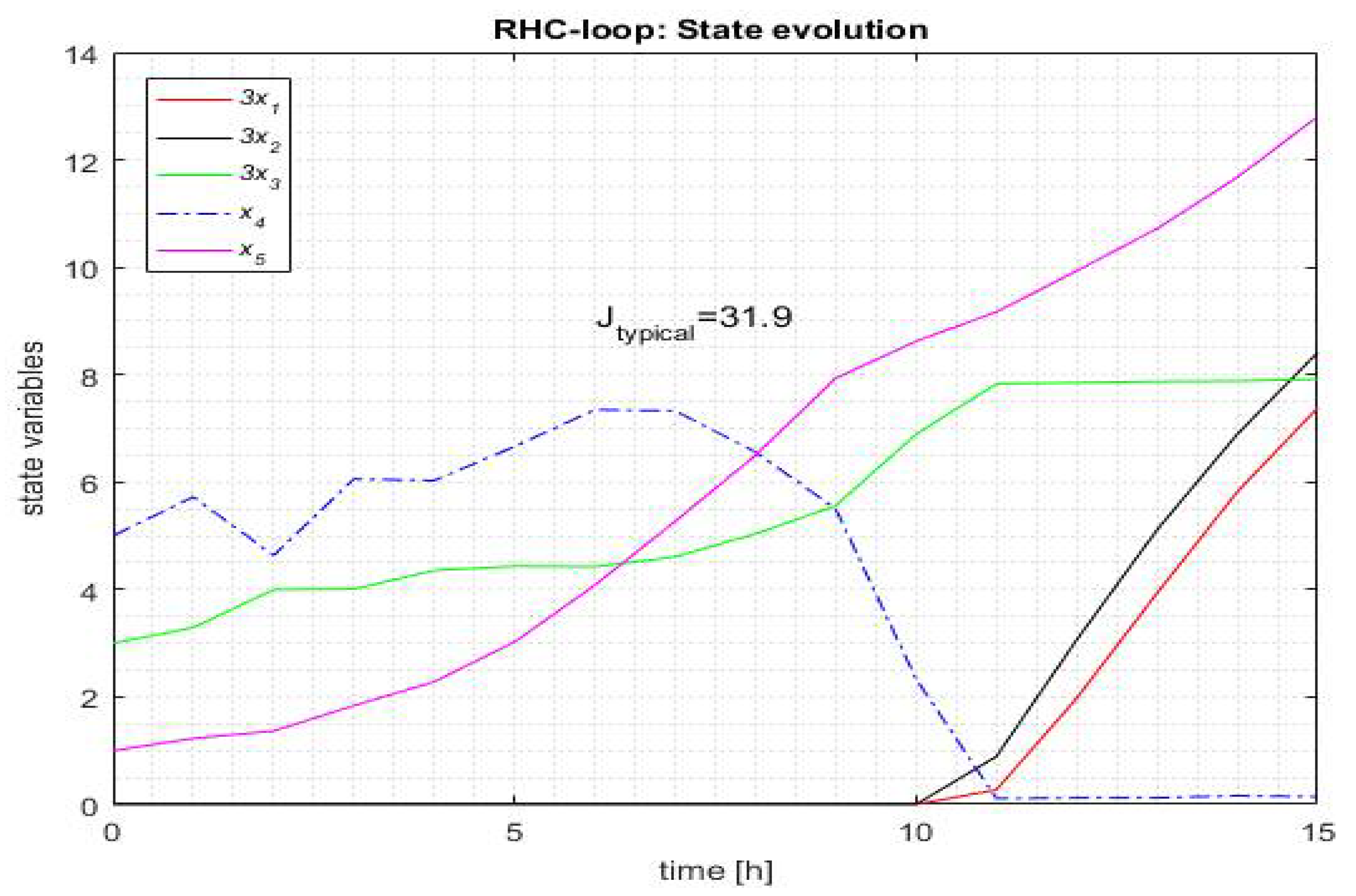
In our simulation series, a specific execution yields Jtypical = 31.900. The other results associated with this run (line 30 in Table 1) are presented hereafter
Jtypical = 31.900; x1(H) = 2.50; x5(H) = 12.74; Ncalls = 6429
The controller calculates the best control output value as the first element of its predicted sequence. These 15 values of the quasi-optimal control output are recorded by the RHC_EA algorithm within the uRHC vector, tracing the controller’s activity over the control horizon. Hence, this vector is not the result of a prediction made at the moment k = 0; in other words, it is not the sequence . This vector allows a final simulation of the closed loop.
The vector uRHC for the typical execution is depicted in Figure 4.
The control outputs of uRHC sent to the Process involve the typical state evolution depicted in Figure 5.
The computational complexity of the first sampling period is the largest because the prediction horizon has H sampling periods. Despite the sequence having an H length, the controller calculates the control variable in a few tens of seconds (depending on processor speed). This duration is quite satisfactory for a sampling period of 1 h.
5.2. Simulation of the Closed Loop with Control Input Range Estimation
In this implementation, ESTIMATOR is called within RHC_EA to reduce the control input range. The “RHC_EA_new.m” program was carried out 30 times for the same instance of the PRP as in the previous section. Practical details about how the simulation results are generated can be found in Appendix D.2.
The new statistic over the 30 runs of the simulation series is given in Table 4.
The typical run corresponds to line #11 of Table 3, Jtypical = 31.887. The other simulation results are presented hereafter
Jtypical = 31.887 x1(H) = 2.357; x5(H) = 13.528; Ncalls = 6030
6. Discussion
We first recall that this work has the same context as that presented in [12]. The basic version of algorithm RHC_EA was created similarly to the previous algorithm (with small differences concerning the EA). We proposed the control input range estimation and compared the closed-loop function in the two algorithm versions, without and with control input range estimation.
The simulations have proved that the RHC_EA program converges for all executions. Aiming to obtain good solutions for PRP and a satisfactory computation time, the predictor stops the iterative process when for the best solution encountered it holds
The stop criterion is either to fulfil constraint (21) or to evolve during Ngen generations. The reported optimum value of J is 32.6, but for algorithms that solve PRP standing alone, not in a closed-loop implementation. As EA now works in a closed loop, its stop-criterion must assure good solutions and adequate execution time for the controller.
Remark 6:
The RHC structure solves a new PRP with a shorter control horizon at each sampling period, starting from the current state vector. Consequently, the values recorded by the uRHC vector are not produced by a single evolutive process (a single run of the EA) for the control horizon [0, H]. That is why the performance index for the control horizon [0, H] is sometimes better than 31.8; the values recorded by the uRHC vector can generate a favorable trajectory.
The main findings of our simulation series are that Figure 5 and Figure 7 ascertain the process has the same quasi-optimal behavior. In the two cases (without and with control input range estimation), the average values of the performance index J are 31.9 and 31.88, respectively. Hence, the ESTIMATOR does not worsen the closed-loop behavior:
- The optimal behavior is not degraded; the two J values are practically identical.
- The process evolutions are very alike.
- The convergence is not impeded.
On the contrary, the RHC_EA algorithm with control input range estimation has a beneficial influence on the computational complexity. Table 5 shows this improvement.
The ratio between the two total numbers of calls (on the entire control horizon) is calculated as
Hence, the computational complexity was diminished by 18.46% using the control input range estimation. This result was expected, but the reduction is large enough considering that range reduction applies only to the first sampling period of the predicted sequences.
The controller meets the time constraint all the more so since the version without ESTIMATOR already fulfils it. Hence, the control structure could be a solution even for real-time control.
In our simulations, we decided that the process is identical to the PM, which is generally not realistic. However, we were interested in seeing the net contribution of the range estimation to the decrease of the computational complexity. If we consider simultaneously perturbative factors (e.g., process PM), the computational complexity will increase to ensure the controller’s optimal character. On the other hand, the papers [9] and [12] treated to a large extent this situation, when process PM, and how simulations can estimate the optimal character degradation.
The ESTIMATOR worked in these simulations having the current state given by the PM. Therefore, it could be useful, at least in simulation studies. In real-time applications, the current state would be given by the real process.
Supplementary Materials
The archive file “ARTICLE_AUTOMATION.zip” contains all files described in Appendix B , Appendix C and Appendix D.
Author Contributions
Conceptualization, V.M.; Methodology, V.M.; Software, I.A.; Validation, V.M.; Formal analysis, V.M.; Investigation, V.M.; Resources, I.A.; Data curation, V.M.; Writing—original draft preparation, V.M.; Writing—review and editing, I.A.; Visualization, I.A.; Supervision, V.M.; Project administration, I.A.; Funding acquisition, V.M.; All authors have read and agreed to the published version of the manuscript.
Funding
This research received no external funding.
Institutional Review Board Statement
Not applicable.
Informed Consent Statement
Not applicable.
Data Availability Statement
The study did not report any data.
Conflicts of Interest
The authors declare no conflict of interest.
Appendix A
Receding Horizon Control
Because the RHC is already well-known, we recall below only the elements that define the RHC strategy:
- The next controller’s output is calculated by looking ahead for several steps in terms of a given cost criterion, but it is only implemented by one step;
- The controller makes predictions for the number of steps taken into account (prediction horizon), using a dynamic PM;
- The controller’s output is sent to the process, and a new decision is made by taking updated information into account and looking ahead for a new prediction horizon.
- The prediction horizon ‘recedes’ at the next sampling period but keeps its final extremity. This is the most difficult situation when the objective function has a terminal penalty term [17]. Hence, the prediction horizon length decreases by one unit at each sampling period.
The RHC structure is depicted in Figure A1, where the notations have the usual meaning. The objective function is denoted in a simplified form by J(, ), where is the sequence of control input values over the prediction horizon that begins at the current moment k. The value u*(k) is the controller’s output sent to the process at the moment k.
Figure A1.
Closed-loop control structure.

The receding horizon controller can use a metaheuristic algorithm to optimize the objective function at hand. A slightly modified EA is integrated into the closed loop in our case. Model predictive control is a special case of RHC when the prediction error is minimized to determine some controller parameters (see [18]). Only the RHC mechanism generates a quasi-optimal solution over the control horizon in this paper. Useful applications concerning the RHC structure are presented in papers [19,20].
Appendix B
Details concerning the ESTIMATOR
Algorithm A1 presents a specific ESTIMATOR implementation adapted to the PRP and the quality criterion chosen in Section 3.1.
| Algorithm A1 | |
| Input parameters: -the initial state ; -length of the estimation interval. Output parameter: | |
| 1 | Initialization of L/* see Equation (15)*/ |
| 2 | ; |
| 3 | forj = 1, …, nv |
| 4 | ; |
| 5 | Compute by integration of system (1) using uk; |
| 6 | ;/*quality criterion Q(j) > 0 */ |
| 7 | end |
| 8 | /* Compute s.t. the interval covers all elements of L that meet the quality criterion*/ |
| 9 | return |
When solving another OCP, line #6 will be modified to deal with another quality criterion.
Line #8 depends on the quality criterion as well. A MATLAB implementation specific to PRP is given by the function “ESTIMATOR_PP.m” inside the folder “ARTICLE_AUTOMATION”.
Figure 1 is generated by the script “drawESTIMATOR.m” that calls the functions “drawFinal6.m” and “EstimateState.m”. These programs are devoted to the analysis made in Section 3.1 and included inside the folder “ARTICLE_AUTOMATION” the lecturer could find in the Supplementary Materials.
Appendix C
Details concerning the EA
Some constant values used by the EA and the mutation function are given below:
- the factor for the left limit of the narrower interval: ;
- technological limits of the control input: ;
- final time: ;
- the minimum value of the performance index: J0 = 31.8;
- number of individuals in the population: N = 35;
- number of children: nr_fii = 30;
- maximum number of generations: NGen = 70;
- selection pressure for the selection operator: s = 1.8;
- the factor that changes the standard deviation: amic = 0.85;
The computation of the objective function (Equation (6)) -specific to PRP-is implemented by the function “eval_PR.m” given inside the folder “ARTICLE_AUTOMATION”. The input parameters are the control input sequence (Equation (8)) and the current state .
Appendix D
Appendix D.1. Simulation Details for RHC_EA without ESTIMATOR
The algorithm RHC_EA is implemented by the script “RHC_EA_new.m”. Line #28 must be updated to turn off the ESTIMATOR: “WithEstimator = 0”. This program can be executed standing alone. “RHC_EA_new.m” was executed 30 times using the script “ciclu30_RHC_EA_new_0.m” and has created the file “WSPmod0.mat”. The script “STATIC_DRAW30_0.m” has computed the statistical parameters presented in Table 1 and Table 2 and generated Figure 4 and Figure 5.
Appendix D.2. Simulation Details for RHC_EA with ESTIMATOR
The algorithm RHC_EA is implemented by the script “RHC_EA_new.m”. Line #28 must be updated to turn on the ESTIMATOR: “WithEstimator = 1”. This program was executed 30 times using the script “ciclu30_RHC_EA_new_1.m” and created the “WSPmod12bis.mat”. The script “STATIC_DRAW30_1.m” has computed the statistical parameters presented in Table 3 and Table 4 and generated Figure 6 and Figure 7.
References
- Kruse, R.; Borgelt, C.; Braune, C.; Mostaghim, S.; Steinbrecher, M. Computational Intelligence—A Methodological Introduction, 2nd ed.; Springer: Berlin/Heidelberg, Germany, 2016. [Google Scholar] [CrossRef]
- Siarry, P. Metaheuristics; Springer: Berlin/Heidelberg, Germany, 2016; ISBN 978-3-319-45403-0. [Google Scholar]
- Talbi, E.G. Metaheuristics—From Design to Implementation; Wiley: Hoboken, NJ, USA, 2009; ISBN 978-0-470-27858-1. [Google Scholar]
- Faber, R.; Jockenhövelb, T.; Tsatsaronis, G. Dynamic optimization with simulated annealing. Comput. Chem. Eng. 2005, 29, 273–290. [Google Scholar] [CrossRef]
- Onwubolu, G.; Babu, B.V. New Optimization Techniques in Engineering; Springer: Berlin/Heidelberg, Germany, 2004. [Google Scholar]
- Valadi, J.; Siarry, P. Applications of Metaheuristics in Process Engineering; Springer International Publishing: Berlin/Heidelberg, Germany, 2014; pp. 1–39. [Google Scholar] [CrossRef]
- Minzu, V.; Riahi, S.; Rusu, E. Optimal control of an ultraviolet water disinfection system. Appl. Sci. 2021, 11, 2638. [Google Scholar] [CrossRef]
- Minzu, V.; Ifrim, G.; Arama, I. Control of Microalgae Growth in Artificially Lighted Photobioreactors Using Metaheuristic-Based Predictions. Sensors 2021, 21, 8065. [Google Scholar] [CrossRef] [PubMed]
- Hu, X.B.; Chen, W.H. Genetic algorithm based on receding horizon control for arrival sequencing and scheduling. Eng. Appl. Artif. Intell. 2005, 18, 633–642. [Google Scholar] [CrossRef] [Green Version]
- Hu, X.B.; Chen, W.H. Genetic Algorithm Based on Receding Horizon Control for Real-Time Implementations in Dynamic Environments. In Proceedings of the 16th Triennial World Congress, Prague, Czech Republic, 4–8 July 2005; Elsevier IFAC Publications: Amsterdam, The Netherlands, 2005. [Google Scholar]
- Goggos, V.; King, R. Evolutionary predictive control. Comput. Chem. Eng. 1996, 20 (Suppl. 2), S817–S822. [Google Scholar] [CrossRef]
- Chiang, P.-K.; Willems, P. Combine Evolutionary Optimization with Model Predictive Control in Real-time Flood Control of a River System. Water Resour. Manag. 2015, 29, 2527–2542. [Google Scholar] [CrossRef]
- Mayne, D.Q.; Michalska, H. Receding Horizon Control of Nonlinear Systems. IEEE Trans. Autom. Control. 1990, 35, 814–824. [Google Scholar] [CrossRef]
- Minzu, V.; Serbencu, A. Systematic procedure for optimal controller implementation using metaheuristic algorithms. Intell. Autom. Soft Comput. 2020, 26, 663–677. [Google Scholar] [CrossRef]
- Banga, J.R.; Balsa-Canto, E.; Moles, C.G.; Alonso, A. Dynamic optimization of bioprocesses: Efficient and robust numerical strategies. J. Biotechnol. 2005, 117, 407–419. [Google Scholar] [CrossRef] [PubMed]
- Balsa-Canto, E.; Banga, J.R.; Aloso, A.V. Vassiliadis. Dynamic optimization of chemical and biochemical processes using restricted second-order information 2001. Comput. Chem. Eng. 2001, 25, 539–546. [Google Scholar] [CrossRef]
- Minzu, V. Quasi-Optimal Character of Metaheuristic-Based Algorithms Used in Closed-Loop—Evaluation through Simulation Series. In Proceedings of the ISEEE, Galati, Romania, 18–20 October 2019. [Google Scholar]
- Abraham, A.; Jain, L.; Goldberg, R. Evolutionary Multiobjective Optimization—Theoretical Advances and Applications; Springer: Berlin/Heidelberg, Germany, 2005; ISBN 1-85233-787-7. [Google Scholar]
- Minzu, V. Optimal Control Implementation with Terminal Penalty Using Metaheuristic Algorithms. Automation 2020, 1, 4. [Google Scholar] [CrossRef]
- Minzu, V.; Riahi, S.; Rusu, E. Implementation aspects regarding closed-loop control systems using evolutionary algorithms. Inventions 2021, 6, 53. [Google Scholar] [CrossRef]
Figure 1.
ESTIMATOR—quality criterion for PRP.

Figure 2.
Receding horizon controller with ESTIMATOR.

Figure 3.
Control input ranges for a prediction horizon.

Figure 4.
Typical control output—controller without control input range estimation.

Figure 5.
Typical state evolution—controller without control input range estimation.

Figure 6.
Typical control output—controller with control input range estimation.

Figure 7.
Typical state evolution—controller with control input range estimation.


Table 1.
Results of the simulation series for RHC_EA without control input range estimation.
| Run # | J | x1(H) | x5(H) | Ncalls | Run # | J | x1(H) | x5(H) | Ncalls |
|---|---|---|---|---|---|---|---|---|---|
| 1 | 31.87 | 2.35 | 13.55 | 8059 | 16 | 31.82 | 2.35 | 13.56 | 6456 |
| 2 | 32.06 | 2.36 | 13.56 | 6121 | 17 | 32.00 | 2.30 | 13.89 | 6063 |
| 3 | 31.80 | 2.47 | 12.86 | 10,718 | 18 | 32.00 | 2.40 | 13.35 | 8065 |
| 4 | 31.90 | 2.34 | 13.66 | 6080 | 19 | 31.81 | 2.45 | 12.99 | 6183 |
| 5 | 32.00 | 2.39 | 13.36 | 6075 | 20 | 32.05 | 2.39 | 13.44 | 9966 |
| 6 | 31.92 | 2.38 | 13.40 | 7240 | 21 | 31.90 | 2.49 | 12.82 | 6465 |
| 7 | 31.82 | 2.33 | 13.64 | 7063 | 22 | 31.84 | 2.30 | 13.85 | 6957 |
| 8 | 31.98 | 2.34 | 13.67 | 9063 | 23 | 31.85 | 2.45 | 13.02 | 8123 |
| 9 | 31.84 | 2.28 | 13.97 | 8497 | 24 | 31.92 | 2.37 | 13.46 | 9138 |
| 10 | 31.89 | 2.35 | 13.55 | 6481 | 25 | 32.02 | 2.36 | 13.59 | 6589 |
| 11 | 31.89 | 2.32 | 13.76 | 7461 | 26 | 32.02 | 2.35 | 13.62 | 6347 |
| 12 | 31.99 | 2.36 | 13.55 | 6828 | 27 | 31.80 | 2.31 | 13.75 | 12,484 |
| 13 | 32.00 | 2.37 | 13.47 | 8633 | 28 | 31.82 | 2.73 | 11.66 | 9160 |
| 14 | 31.83 | 2.38 | 13.36 | 10,788 | 29 | 31.85 | 2.34 | 13.59 | 7932 |
| 15 | 31.83 | 2.42 | 13.18 | 7415 | 30 | 31.90 | 2.50 | 12.74 | 6429 |
Table 2.
Statistic regarding the optimum criterion.
| Jmin | Javg | Jmax | Sdev | Jtypical |
|---|---|---|---|---|
| 31.800 | 31.908 | 32.058 | 0.142 | 31.900 |
Table 3.
Results of the simulation series for RHC_EA with control input range estimation.
| Run No. | J | x1(H) | x5(H) | Ncalls | Run # | J | x1(H) | x5(H) | Ncalls |
|---|---|---|---|---|---|---|---|---|---|
| 1 | 31.859 | 2.318 | 13.744 | 5686 | 16 | 31.799 | 2.495 | 12.745 | 7121 |
| 2 | 32.067 | 2.375 | 13.502 | 5675 | 17 | 31.797 | 2.390 | 13.302 | 7868 |
| 3 | 31.925 | 2.343 | 13.628 | 6739 | 18 | 31.854 | 2.258 | 14.104 | 5582 |
| 4 | 31.837 | 2.312 | 13.771 | 5474 | 19 | 31.871 | 2.487 | 12.814 | 6057 |
| 5 | 31.840 | 2.284 | 13.943 | 6698 | 20 | 32.004 | 2.375 | 13.478 | 7775 |
| 6 | 31.947 | 2.319 | 13.778 | 4350 | 21 | 31.888 | 2.335 | 13.657 | 5531 |
| 7 | 31.925 | 2.375 | 13.442 | 5956 | 22 | 31.931 | 2.332 | 13.695 | 5979 |
| 8 | 31.818 | 2.515 | 12.651 | 7168 | 23 | 31.666 | 2.236 | 14.162 | 10,063 |
| 9 | 31.806 | 2.434 | 13.070 | 6600 | 24 | 31.867 | 2.466 | 12.921 | 7246 |
| 10 | 32.026 | 2.345 | 13.657 | 6439 | 25 | 31.841 | 2.526 | 12.607 | 6177 |
| 11 | 31.887 | 2.357 | 13.528 | 6030 | 26 | 31.812 | 2.417 | 13.164 | 5294 |
| 12 | 31.872 | 2.352 | 13.551 | 5679 | 27 | 31.843 | 2.415 | 13.185 | 7216 |
| 13 | 32.047 | 2.341 | 13.689 | 5242 | 28 | 31.909 | 2.372 | 13.451 | 5610 |
| 14 | 31.909 | 2.529 | 12.619 | 4862 | 29 | 31.812 | 2.346 | 13.563 | 6832 |
| 15 | 31.851 | 2.486 | 12.813 | 5982 | 30 | 31.895 | 2.407 | 13.252 | 6962 |
Table 4.
New statistic regarding the optimum criterion over the 30 runs.
| Jmin | Javg | Jmax | Sdev | Jtypical |
|---|---|---|---|---|
| 31.666 | 31.880 | 32.067 | 0.00687 | 31.887 |
Table 5.
Objective function’s calls number over 30 runs.
| Ncallsmin | Ncallsavg | Ncallsmax | Sdev | |
|---|---|---|---|---|
| without ESTIMATOR | 6063.4 | 7762.57 | 12,483.8 | 1647 |
| with ESTIMATOR | 4349.8 | 6329.8 | 10,063. | 1099 |
Publisher’s Note: MDPI stays neutral with regard to jurisdictional claims in published maps and institutional affiliations. |
© 2022 by the authors. Licensee MDPI, Basel, Switzerland. This article is an open access article distributed under the terms and conditions of the Creative Commons Attribution (CC BY) license (https://creativecommons.org/licenses/by/4.0/).
Share and Cite
MDPI and ACS Style
Mînzu, V.; Arama, I. Optimal Control Systems Using Evolutionary Algorithm-Control Input Range Estimation. Automation 2022, 3, 95-115. https://0-doi-org.brum.beds.ac.uk/10.3390/automation3010005
AMA Style
Mînzu V, Arama I. Optimal Control Systems Using Evolutionary Algorithm-Control Input Range Estimation. Automation. 2022; 3(1):95-115. https://0-doi-org.brum.beds.ac.uk/10.3390/automation3010005
Chicago/Turabian StyleMînzu, Viorel, and Iulian Arama. 2022. "Optimal Control Systems Using Evolutionary Algorithm-Control Input Range Estimation" Automation 3, no. 1: 95-115. https://0-doi-org.brum.beds.ac.uk/10.3390/automation3010005