Article

Modeling County-Level Energy Demands for Commercial Buildings Due to Climate Variability with Prototype Building Simulations

1
Department of Atmospheric Sciences, University of Utah, Salt Lake City, UT 84112, USA
2
Pulmonary Division, School of Medicine, University of Utah, Salt Lake City, UT 84112, USA
3
Department of City & Metropolitan Planning, University of Utah, Salt Lake City, UT 84112, USA
4
Department of Mechanical Engineering, University of Utah, Salt Lake City, UT 84112, USA
5
Commercial Buildings Research Group, National Renewable Energy Laboratory, Golden, CO 80401, USA
*
Author to whom correspondence should be addressed.
Submission received: 19 June 2020 / Revised: 11 July 2020 / Accepted: 22 July 2020 / Published: 23 July 2020

Abstract

:
The building sector accounts for nearly 40% of total primary energy consumption in the U.S. and E.U. and 20% of worldwide delivered energy consumption. Climate projections predict an increase of average annual temperatures between 1.1–5.4 °C by 2100. As urbanization is expected to continue increasing at a rapid pace, the energy consumption of buildings is likely to play a pivotal role in the overall energy budget. In this study, we used EnergyPlus building energy models to estimate the future energy demands of commercial buildings in Salt Lake County, Utah, USA, using locally-derived climate projections. We found significant variability in the energy demand profiles when simulating the study buildings under different climate scenarios, based on the energy standard the building was designed to meet, with reductions ranging from 10% to 60% in natural gas consumption for heating and increases ranging from 10% to 30% in electricity consumption for cooling. A case study, using projected 2040 building stock, showed a weighted average decrease in heating energy of 25% and an increase of 15% in cooling energy. We also found that building standards between ASHRAE 90.1-2004 and 90.1-2016 play a comparatively smaller role than variation in climate scenarios on the energy demand variability within building types. Our findings underscore the large range of potential future building energy consumption which depends on climatic conditions, as well as building types and standards.

1. Introduction

1.1. Motivation

Buildings are responsible for approximately 40% of total primary energy consumption in the U.S. and E.U. [1] and for 20% of worldwide delivered energy consumption [2,3]. By 2050, 66% of the world population, and 82% of North America, are predicted to be living in urban environments, increasing the amount of energy consumed by buildings in cities [4]. Nevertheless, the relative impact of building energy consumption as a percentage of total delivery energy worldwide is projected by the U.S. Energy Information Administration to be constant between 2012 and 2040, as shown in Figure 1 [5].
These consumption scenarios primarily focus on economic growth for predicting future building energy consumption, but the report acknowledges the importance of energy-related components of climate pledges in advance of the 2015 Paris Climate Change Conference (COP21) [6]. However, according to a National Oceanic and Atmospheric Administration (NOAA) report, world average temperature is projected to increase by 2100 by 1.1 °C to 5.4 °C [7]. De Wilde and Coley describe the link between climate and buildings: “Buildings provide an interface between the outdoor environment, which is subject to climate change, and the indoor environment, which needs to be maintained within a range that keeps the occupants safe and comfortable, and which is suitable for any key processes that are taking places within the building” [8]. An increase in air temperature will have a significant impact on building energy consumption worldwide, increasing the cooling energy demand and reducing the heating energy demand.

1.2. Literature Review and Previous Work

Several studies in the literature have focused on the impact of climate variability on building energy consumption, including a recent review [9]. Using results from the Low Carbon Futures (LCF) and Adaptation and Resiliency In Energy Systems (ARIES) projects, a study presented potential outcomes on the provision and use of energy in buildings associated with a changing climate [10]. Netherlands [11], Norway [12], China [13,14], UK [15], Greece [16], India [17], Australia [18], Italy [19,20,21], Iran [22], and the USA [23,24].
The same climatic shift affects different locations differently, with impacts not only on the building energy consumption, but on the electric power grids. A study found that rising global temperatures will result in increased cooling needs in Swiss buildings leading to significant impacts on building designs and on the electric demand on the Swiss power grid. [25]. Similarly, in the U.S., given the high use of AC systems, climatic warming will increase the electric peak on the power grid by between 4.2% to 15% [26]; possibly more than estimated, given the non-linear relationship between dry bulb temperature and relative humidity [27].
Some researchers have used parametric methods to estimate building energy consumption, such as the heating degree days (HDD) and cooling degree days (CDD), in the context of the balance-point method for energy analysis. However, using the “fixed” balance point method was found to overestimate the energy consumption in most American states [28]. Another study investigated establishing energy benchmarks for both existing and new building types in order to quantify the impact of various intervention strategies [29].
The use of building energy modeling (BEM), therefore, seems a logical and necessary methodology to analyze the impact of future climate on building energy consumption. This approach consists of using computer-based tools to model and analyze building energy consumption, under different climate boundary conditions [30,31]. A recent study employed EnergyPlus to estimate building energy consumption, on a district level, under future climate scenarios; however, this analysis was focused on one building model only, a small office [32]. A multi-city study used EnergyPlus to understand the impacts of climate change in building energy use in Miami, Baltimore and Boston [33]. However, only two building types were used and a wider variety of building types would be required to accurately represent the building stock in a city. A campus energy study used five representative EnergyPlus models to analyze the implications of future climate changes on total energy consumption, heating and cooling energy consumption, and peak electric demand for the University of Michigan, demonstrating the usefulness of aggregating building archetypes and simulating them within a particular spatial area to understand the response to future weather under different climate scenarios [34].
Bianchi et al. [35] previously analyzed the impact of climate variability on three commercial building types and a central business district area comprised of one block of downtown Salt Lake City. They highlighted the importance of considering building design and building types. In their analysis, however, they used projected weather data based on global NOAA predictions [7]. It is therefore necessary to perform building energy simulations with climatic predictions tailored for a study location, in this case, Salt Lake County, in order to have a more reliable starting point to model future building energy consumption, particularly under a changing climate [28,36].
Future building stock is a necessary component in estimating the impact of offsetting factors associated with primary energy use. Thus, engineering models used in conjunction with a large statistical sample of buildings (i.e., the Commercial Buildings Energy Consumption Survey or CBECS) are a useful combination for projection models [37]. It is important, therefore, to use multiple building types while also considering the likely distribution of building types in the projected building stock for future years. Furthermore, the use of building prototypes is a well-established technique to quantify potential energy savings [38].
U.S. Department of Energy researchers have investigated the impact of climate change on energy consumption of buildings for over a quarter century [27], and many researchers have been using BEM software to run models that link changes in energy use to changes in weather. “It appears beneficial to obtain a more detailed understanding of how advanced design in different building types would behave with global warming” [27] (p. 331). The same building type reacts to the same climatic variation differently, depending on its specific design.

1.3. Significance of This Work

This study builds on and adds to the previous work in literature in the following ways:
  • We used localized weather data specific to an urban area (Salt Lake County), developed by a team of atmospheric scientists, accounting for site-specific future projections as input for building energy simulations instead of average climate trends modeled for the whole country or the world.
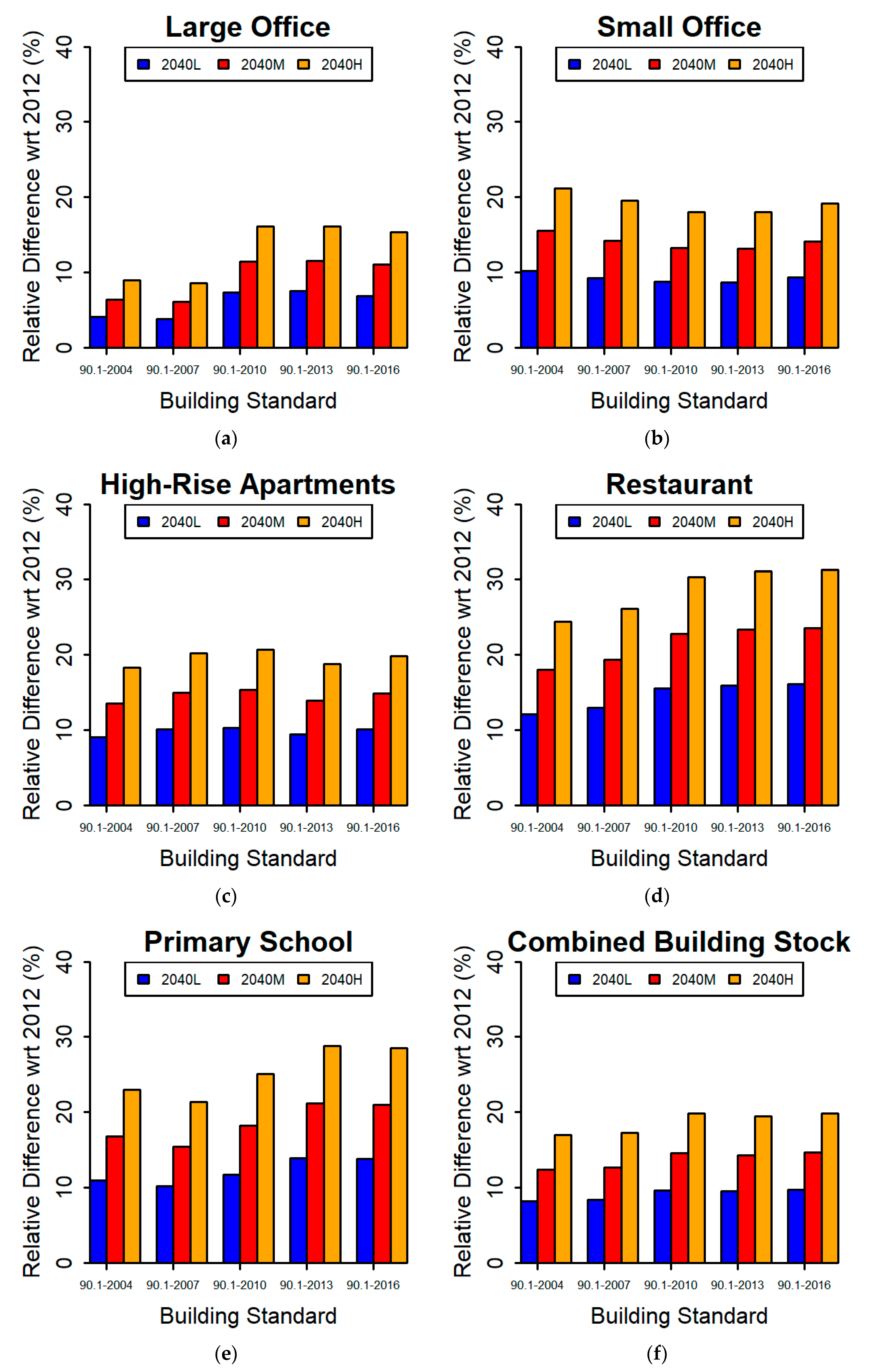
  • We used multiple building stock models, representing five commercial building types, in order to understand how a given variation in dry bulb temperature affects different building types. This study includes the five commercial building types most prevalent in the study area (large office, small office, primary school, full-service restaurant, and high-rise multi-family apartment buildings) collectively comprising 49% and 55% of the floor area of existing and projected future building stock, respectively [39].
  • We included multiple building energy standards (ASHRAE 90.1-2004, 2007, 2010, 2013 and 2016) to understand how a given variation in dry bulb temperature affects a given building type when built to meet different design standards.
  • We considered the projected 2040 composition of Salt Lake County’s building stock to have a more realistic prediction of aggregated commercial building energy consumption.
Previous studies, including those listed in Section 1.2, have included individual components outlined above, but, to the authors’ knowledge, this is the first study to combine these elements. Furthermore, since a representative amount of building stock is considered, micro-climate effects, such as urban heat islands, are not explicitly modeled.
The rest of this manuscript is structured as follows: Section 2 describes the materials and methods, Section 3 presents the results, Section 4 provides a discussion of the findings, and Section 5 draws conclusions gained from this study.

2. Materials and Methods

Building energy consumption was simulated for stock building models using actual 2012 observed weather data and three 2040 projected climate scenarios weather files using EnergyPlus [40]. The cooling and heating loads, as well as electricity and natural gas consumption, were taken from the energy model simulation output for five commercial building types (large office, small office, primary school, full-service restaurant, and high-rise multi-family apartment buildings) as built to five different energy standards (ASHRAE 90.1-2004, 90.1-2007, 90.1-2010, 90.1-2013 and 90.1-2016).

2.1. Weather Data for Energy Modeling

The meteorological conditions for 2040 were developed by modifying the 2012 hourly temperature and relative humidity readings from the Salt Lake City Airport (KSLC) with the utilization of three climate change scenarios based on the Coupled Model Intercomparison Project Phase 5 (CMIP5) [41,42]. CMIP is a sophisticated climate model that incorporates both unforced variability and changes in radiative forcing to develop future projections. These scenarios were classified as “Low”, “Mean”, and “High” according to the modeled temperature increase. The heating degree days (HDD) and cooling degree days (CDD) were calculated using 65 °F (18.3 °C) as the base temperature.

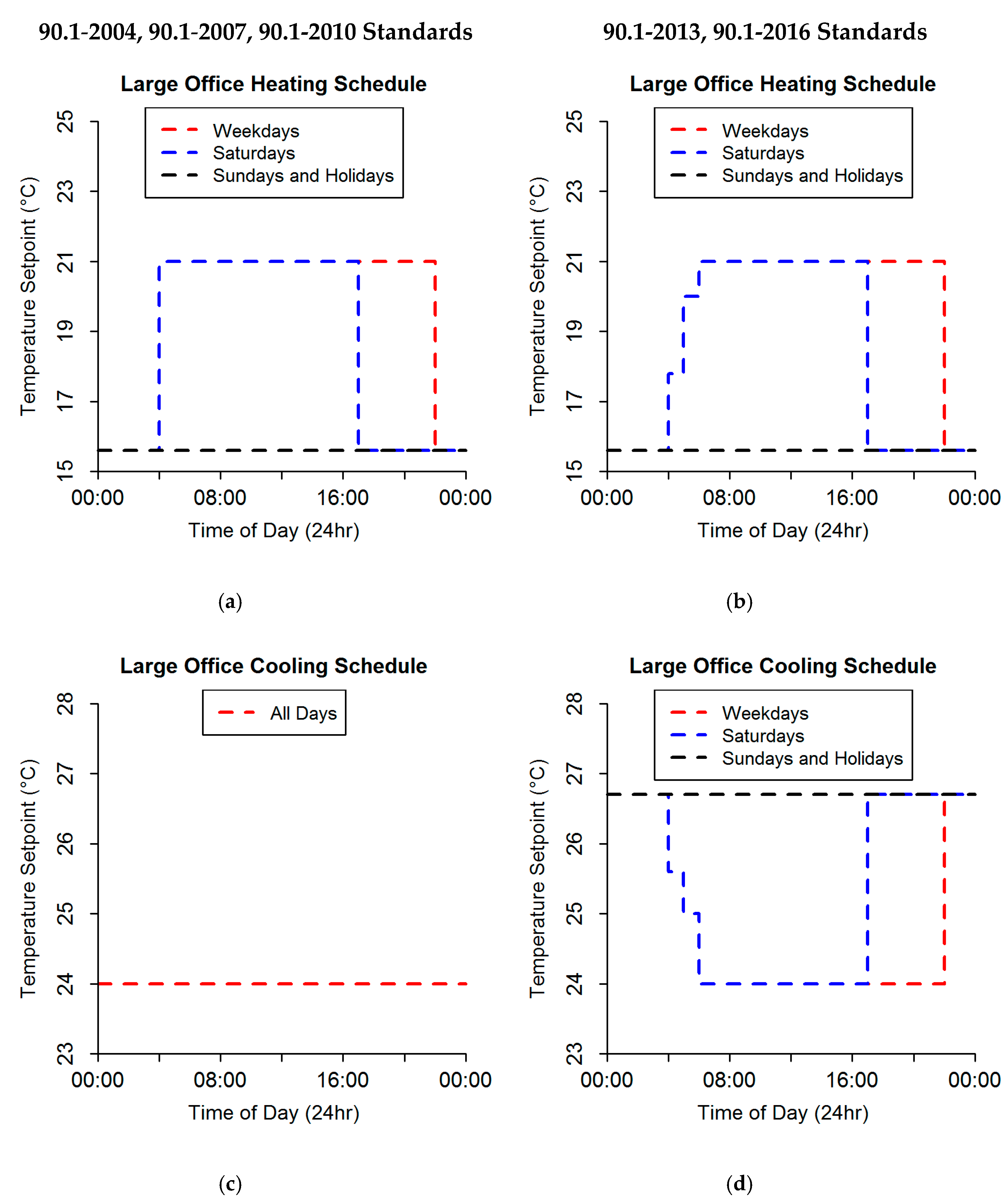
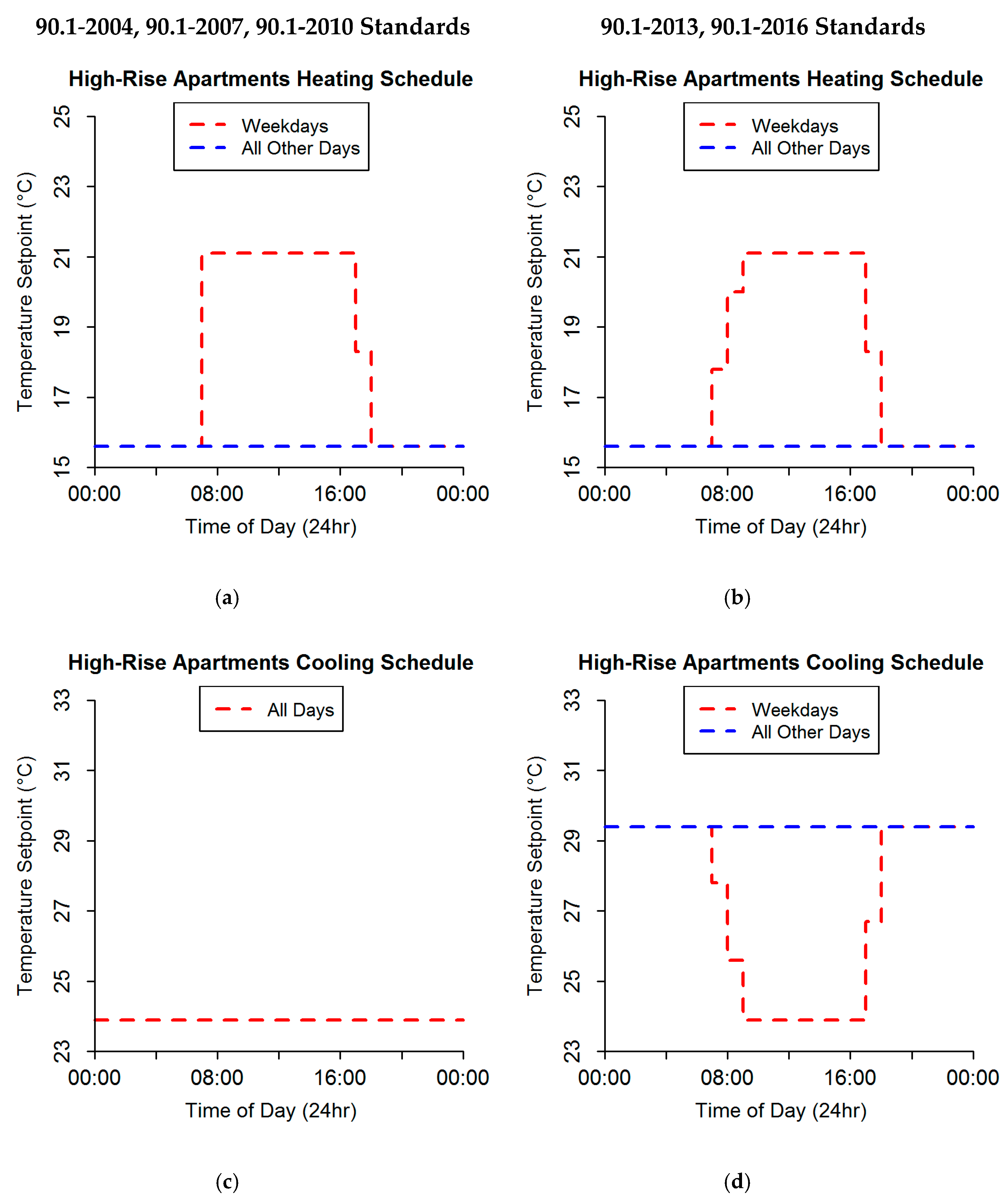
2.2. Building Simulations

EnergyPlus [40] was used to run the building energy simulations. The EnergyPlus simulation engine is a U.S. Department of Energy-supported building energy modeling program and is well documented, validated, and open-source. EnergyPlus requires a weather file to simulate the meteorological conditions during the period of simulation and an input data file to describe the building being simulated. For this study, the weather files were used as mentioned in Section 2.1. Commercial prototype building models [43] were used to represent the building stock selected for simulation [38]. The commercial prototype building models used were designed for Denver, Colorado, USA, the nearest available city in the same International Energy Conservation Code (IECC) climate zone (5B) as Salt Lake City, Utah [44]. The commercial prototype models were created by Pacific Northwest National Laboratory (PNNL) for the EnergyPlus version 8.0 [40] engine, and therefore, EnergyPlus 8.0 was used for the simulations. The buildings simulated were the Small Office, Large Office, Full-Service Restaurant, Primary School, and High-Rise prototype building models—all of which are classified as commercial buildings by the U.S. Department of Energy [43]. The commercial prototype building models were designed to represent buildings that would meet ASHRAE Standard 90.1 (Energy Standard for Buildings Except Low-Rise Residential Buildings) for the 90.1 Versions for 2004, 2007, 2010, 2013, and 2016.
Addendum cb to Standard 90.1-2010 [45] added new requirements and clarification to the setback and optimal start control requirements for building HVAC systems. As a result, the published prototype models conforming to Standards 90.1-2013 and 90.1-2016 have new setback and optimum start control strategies in the form of thermostat schedule modifications which are different from the thermostat schedules used for the prototype models conforming to Standards 90.1-2004, 90.1-2007 and 90.1-2010 [46]. A detailed example of changes that were implemented in the thermostat scheduling because of Addendum cb Standard 90.1-2010 can be found in Appendix A.
During our EnergyPlus simulation runs, we found significant variations in results, occurring because of the thermostat schedule modifications. To provide consistency in results between different ASHRAE 90.1 Standard years, we chose to make the schedules uniform among the compared prototype building models so that the results would reflect changes in the buildings themselves and not changes in the operational strategies. The thermostat schedule used in the prototype models for Standards 90.1-2004, 2007 and 2010 (as shown in Appendix A) was chosen and it replaced the new schedules that had been in the published prototype models for Standards 90.1-2013 and 2016. All results presented below have been simulated using a uniform thermostat schedule taken from the prototype models for Standards 90.1-2004, 2007 and 2010.
The modification was done by:
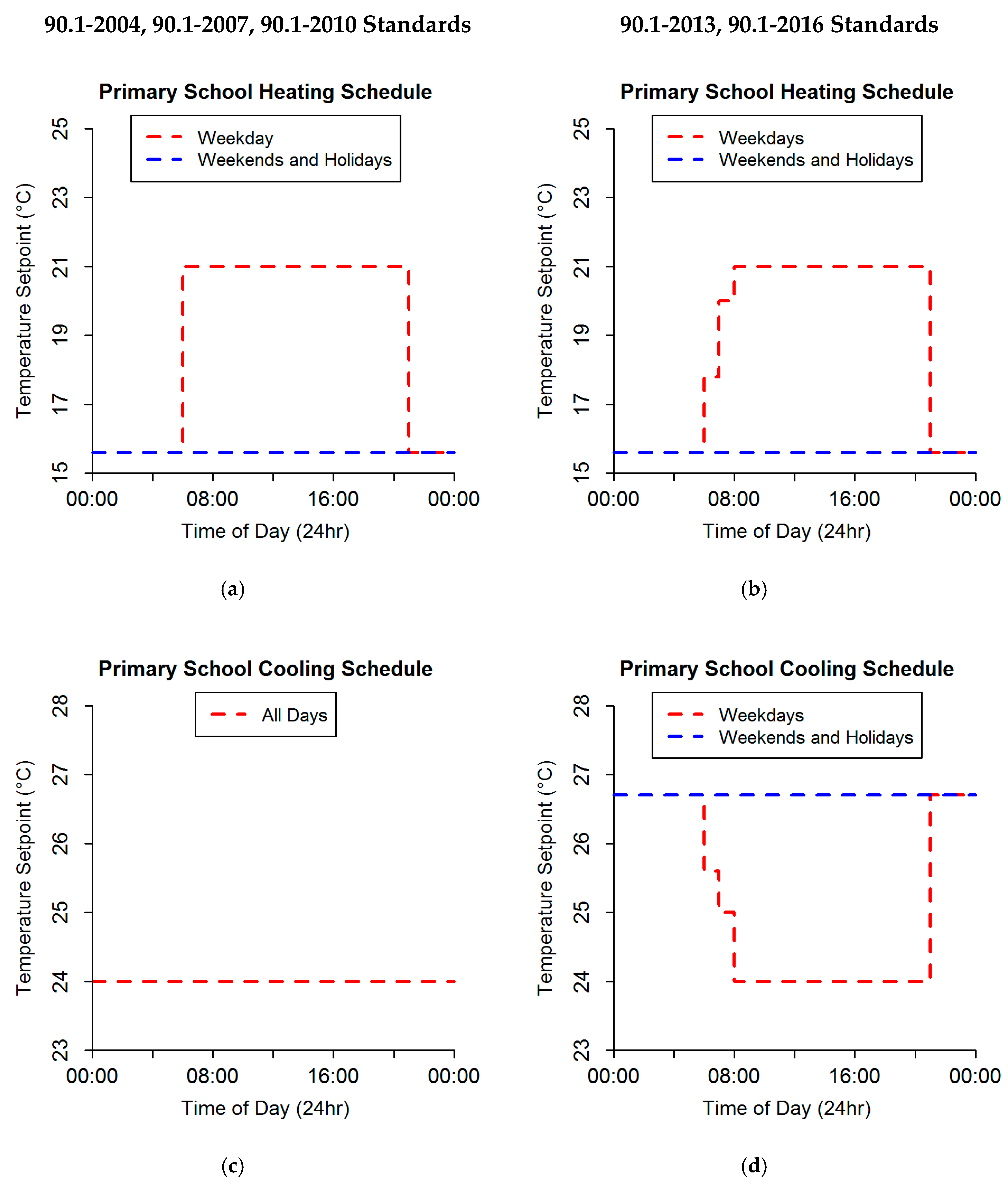
  • Searching for thermostat schedule changes in the input data files (IDFs) between the published Standard 90.1-2004, 90.1-2007 and 90.1-2010 and the published Standard 90.1-2013 and 90.1-2016 prototype models.
  • Replacing the thermostat schedules that were different in the Standard (90.1-2013 and 90.1-2016) prototype models with the respective thermostat schedules in Standard (90.1-2004, 90.1-2007 and 90.1-2010) prototype models.
In order to compare the impact of climate on building conditioning (HVAC) energy consumption, two resulting EnergyPlus output metrics were compared:
  • Heating:Gas—This metric includes gas used by boilers, direct exchange coils that provide supplementary heating to heat pumps, and gas use by main gas heating coils.
  • Cooling:Electricity—This metric includes electricity consumption due to heat pumps working in cooling mode and chiller electric energy as well as electricity consumed by direct exchange cooling coils.

2.3. Salt Lake County Case Study

Salt Lake County is a rapidly developing urban center with a population expected to grow by almost 50%, from 2010 baseline levels, by 2040 [47]. The regional metropolitan planning organization, the Wasatch Front Regional Council (WFRC), has developed future land use scenarios for 2040 in support of its regional transportation plan [48]. The 2012 and projected 2040 square footage by building type are shown in Table 1. The 2012 square footage of the five study building types accounts for 49% of built area and will rise to nearly 55% by 2040. Therefore, estimating the energy demand changes for these five building types can provide a substantially representative change in energy demand for Salt Lake County.

3. Results

3.1. Contemporary and Future Meteorological Conditions

The means and standard deviations for the historical and projected meteorological scenarios, along with the percent change from the 2012 baseline, are shown in Table 2. The increase in mean temperature ranges from 0.9–2.3 °C compared to the baseline temperature. This is comparable to projections from NOAA [7].
Heating and cooling degree days for each of the four study scenarios using 65 °F (18.3 °C) as the base temperature are listed in Table 3. The percent change from the 2012 baseline was also calculated for the three projected meteorological scenarios. The decrease in HDD modestly outpaced the mean temperature increase (Table 2) for the Low and Medium scenarios (~1–4%) but was much more noticeable for the High scenario (~8%). The increase in CDD was approximately 8–9% higher than the decrease in HDD for all scenarios. This divergence in the impact of modeled temperature scenarios on CDD/HDD shows that these are non-linear functions and will disproportionately affect energy demands during the summer compared to the winter.

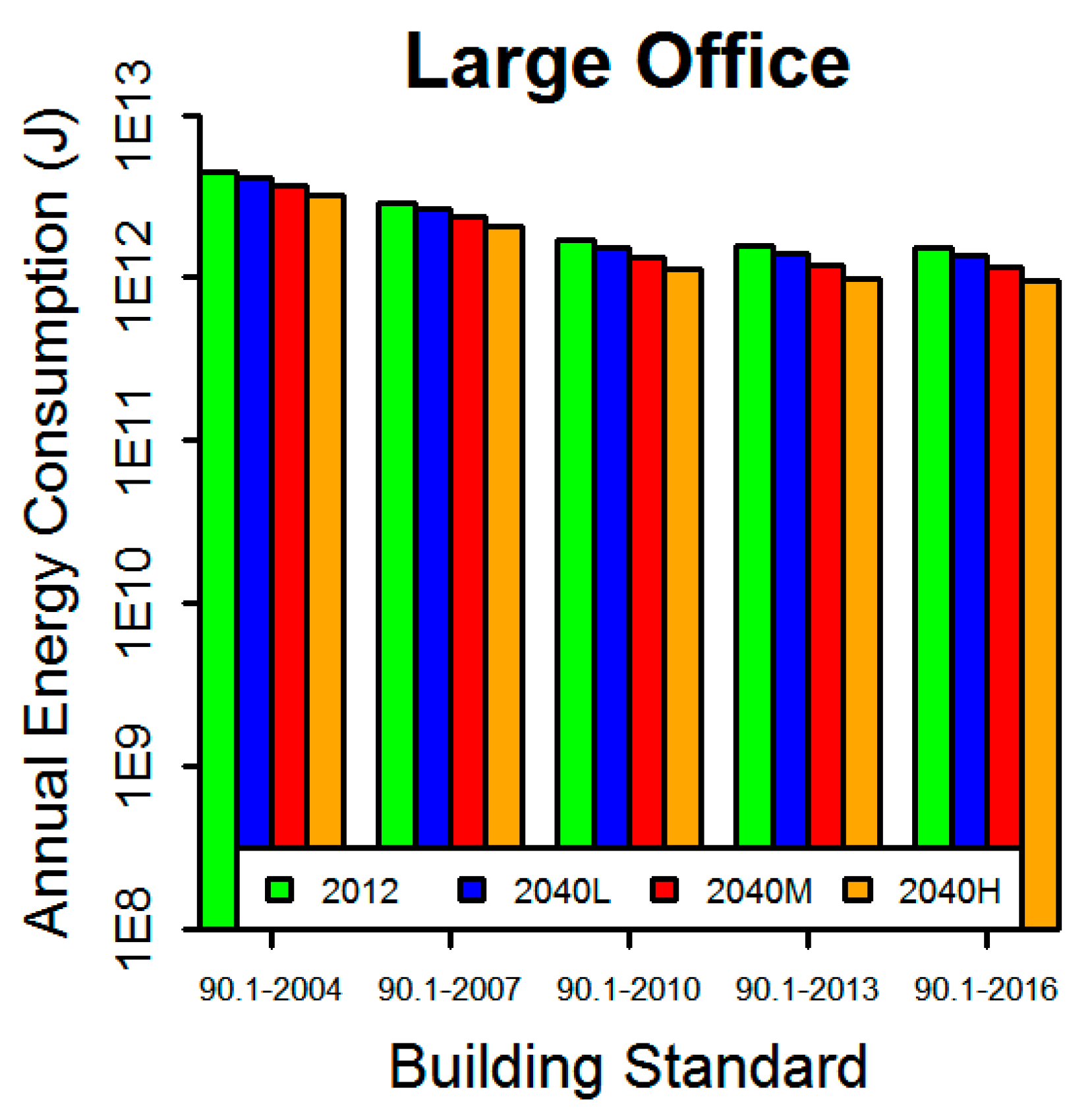
3.2. Results of Building Simulations

3.2.1. Heating Natural Gas Consumption

The annual heating natural gas consumption and relative differences, with respect to 2012, for the three meteorological scenarios for the study building types and standards are shown in Figure 2, Appendix B, and Figure 3. The modeled 2040 meteorological scenarios result in lower natural gas consumption for all building types and standard combinations, due to the lower demand for heating. The office building type shows the two largest relative decreases in 2040 heating energy with respect to the 2012 baseline, with large offices (Figure 3a) and small offices (Figure 3b) reaching reductions of up to 30% and 75%, respectively. The high-rise apartment, restaurant, and primary school building types (Figure 3c–e) showed relatively minor differences in natural gas consumption between the building standards. High-rise apartment buildings (Figure 3c) show consistently smaller relative gas consumption reductions across the building standards; however, as their share of the built area is expected to be approximately a quarter of that taken up by the commercial sector, these reductions are not negligible. Restaurants (Figure 3d) showed a nearly constant pattern of gas consumption reduction across building standards. It must be noted that only approximately 40% of natural gas consumed by restaurants is used for heating, while the majority is used for other purposes, primarily cooking, which will not be directly affected by the meteorology. Throughout all cases, more modern building standards result in lower absolute natural gas consumption regardless of the scenario (Figure 2, Appendix B). While the small office and primary school building types (Figure 3b,e) show the largest percentage reductions, from 2012 baseline levels, for the 90.1-2010 Standard, the newer Standards (90.1-2013 and 90.1-2016) still result in lower absolute natural gas consumption. The energy demand of the combined building stock (composed of these five building types which are expected to represent nearly 55% of the commercial building stock by 2040) is reflective of the two largest contributors: high-rise apartments and large offices (Figure 3f).

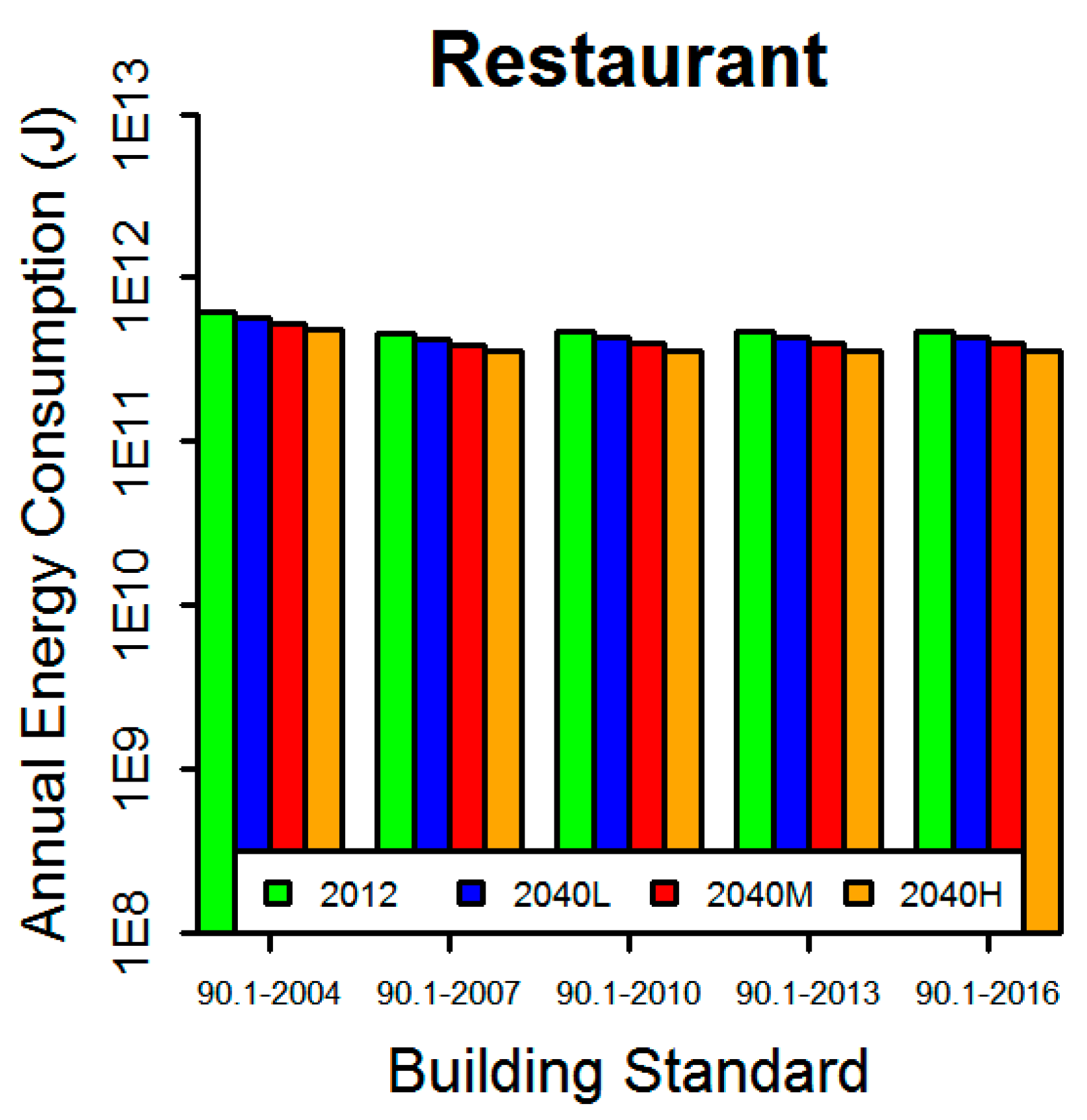
3.2.2. Cooling Energy Consumption

The annual cooling electricity consumption and relative differences, with respect to 2012, for the three meteorological scenarios for the study building types and standards are shown in Figure 4, Appendix C, and Figure 5. Appendix D describes in detail the differences across building standards. For all building types, the relative cooling electricity consumption differences for the different meteorological and building standards are approximately of the same magnitude as the natural gas consumption differences (Figure 3). However, the opposite pattern is found where higher temperature scenarios require a larger increase in electricity consumption to provide for the cooling needs of the buildings. The large office building type (Figure 5a) shows the highest relative increase in cooling electricity consumption when built to the 90.1-2010 or 90.1-2013 building standards, with a small decrease for the 90.1-2016 Standard. Small offices and high-rise apartments (Figure 5b,c) show a decrease in relative cooling electricity consumption for newer building standards. This could be interpreted as buildings built to newer standards are less affected by increasing temperatures. Restaurants and primary schools (Figure 5d,e) display a counter-intuitive pattern where the newer building standards are more affected by increasing temperatures. However, the absolute electricity consumption consistently decreases for newer building standards for all temperature scenarios including the 2012 baseline. Therefore, while a relative increase may be larger percentagewise, the net consumption (Figure 4 and Appendix C) consistently decreases for newer standards. In a similar manner as for the heating analysis, the combined building stock results (Figure 5f) are reflective of the contributions from large office and high-rise apartments (Figure 5a,c) with a small contribution from the restaurant buildings (Figure 5d).

4. Discussion

4.1. Meteorological Variability

The temperature changes expected to take place by 2040 are substantial compared to the 2012 baseline. The lowest climatic change scenario (2040L) yields an increase in average with an annual of 0.9 °C, the highest (2040H) of 2.3 °C, and the most likely (2040M) of 1.6 °C (Table 2). The effects of the projected temperature increase result in substantial changes to HDD and CDD (Table 3). While the lower and medium scenarios show comparable effects in HDD and CDD, the high scenario shows a substantially higher impact on HDD and CDD. These findings underscore the resulting temperature extremes, not just average temperature changes, attributable to increased warming trends, and serve as a sensitivity analysis of energy consumption in relationship to temperature.

4.2. Building Energy Consumption

The projected temperature increases result in reduced HDD and corresponding natural gas consumption across all 2040 meteorological scenarios (Figure 3). The small and large office building types show the largest natural gas consumption decreases of up to 75% and 30%, respectively, when modeled to meet several ASHRAE 90.1 Building Standards. Together, these two building types are projected to account for nearly a quarter of the total building stock, by square footage, in 2040, therefore having a significant impact on heating energy consumption. The high-rise apartment buildings, which will also account for approximately a quarter of built square footage, show markedly lower reductions in the range of 10%.
On the other side of the energy consumption balance, restaurants and schools are projected to increase their cooling electricity demands by up to 30% (Figure 5). However, these two building types are only expected to account for a little over 8% of the building stock by 2040. High-rise apartments and both small and large office building types, accounting for approximately half of all building stock, will increase their cooling electricity demands by approximately 20%. Therefore, a large fraction of the built environment will need significantly larger amounts of electricity to maintain functionality.
A significant finding of this study is the large range of energy consumption variability across buildings. Across all building types, there is a greater relative reduction in energy consumption for heating needs compared to the increase in cooling needs. However, the absolute magnitude of energy consumption can vary by up to a factor of 10 when comparing heating and cooling needs, such as for the restaurant building type (Figure A8 and Figure A12).

4.3. Case Study Findings

The case study of projected Salt Lake County commercial building energy demands shows the strong influence of the building types projected to have the largest floor area by square footage: high-rise apartments and offices. The model results show that the impact of future climate on reduced heating consumption is, percentagewise, similar to the impact on increased cooling consumption, approximately 15% relative to 2012 consumption for the combined building stock, which accounts for 55% of the projected built environment in Salt Lake County. The small office building type is the most sensitive to future climatic conditions, both cooling and heating; however, due to its comparatively smaller contribution to the overall building stock, its influence is less reflected at the county level.

5. Conclusions

5.1. Implications

This study found that building energy consumption will vary substantially due to modeled temperature increases. With a decrease in heating degree days and an increase in cooling degree days, natural gas consumption is expected to decrease while electricity consumption is expected to increase, based on currently available technologies where natural gas is the primary heating source and electricity is used for cooling. These effects were found to vary significantly across building types with small offices showing the largest decreases in natural gas consumption and schools showing the largest increases in cooling electricity consumption. Building standards play a significant role in projected energy demands with large offices showing the largest variability dependence on building standards. This suggests that potential building energy savings due to retrofits can vary widely depending on climatic conditions, and building types and standards, as found in previous studies [49]. The reductions in local emissions due to lowered heating demand may have a potentially large positive impact on local air quality. Conversely, additional electricity demand may have a negative air quality impact, but this may not directly affect the local airshed since the primary electricity generating facilities are located outside the study area. In this study, we have shown that, due to the large differences, both in absolute and relative terms, the energy demands of future urban development is noticeably sensitive to building type growth.

5.2. Limitations

There are several limitations to this study, primarily because it is a predictive study with several implied assumptions used. Climate variability is a large unknown, and as the largest energy consumption driver, may result in substantially different outcomes if future weather changes in ways that were not captured in these scenarios. Our analysis assumes no variation in cloud coverage for the future climate scenarios. In the literature, some works have studied how cloud coverage, and therefore, solar irradiation, will change in the future [50]; however, the IPCC models did not include major changes in the cloud coverage. Future developments of our work will include this aspect for a more complete analysis. In this study, we used the available building year standards (up to 2016), but no future technology scenarios or scheduling are modeled, meaning that the impacts of increasingly efficient equipment that is adopted in the future or the use of advanced control methodologies would not be captured. Salt Lake County is developing rapidly but no additional heat island effects were accounted for in this study. Although the buildings studied represent the majority (55%) of the projected 2040 building stock, not all building types were included in the analysis. Additionally, building energy simulations do not provide exact numbers for the magnitude of energy consumption, but rather are used to represent relative changes, and they use a large number of underlying assumptions about how the parameters for the EnergyPlus prototype models were chosen. Although the diversification of the building stock assumed in this work represents the real Salt Lake Valley building diversification, each building model was not calibrated to represent a real building. Lastly, micro-climate effects, such as urban heat islands, are not explicitly modeled in this study. Urban heat islands (UHIs) play an important role on building energy performance in urban areas. The authors have previously published on the presence of UHIs in the Salt Lake Valley [51]. The presented analysis does not include any UHI effect on the results. UHI effect would increase the impact of climate change in urban areas with respect to what is described in this work. Future developments of our work will include this aspect for a more complete analysis. The focus of the present study was to estimate the impact of a changing climate on the larger building stock cohort for Salt Lake County, without the inclusion of specific building geometry.

5.3. Future Work

Future directions for this study include performing a similar analysis on residential buildings, which tend to have energy use highly impacted by the weather. The urban heat island effect, magnified due to the rapid urbanization taking place in Salt Lake County, may play a significant role in overall energy consumption, and further work may enable the quantification of this effect. Other building energy models could be used to calibrate and provide formal uncertainty estimates for these findings. A complementary avenue of research would be to contextualize the cooling and heating energy demands within the overall building energy budget. With rapid technological change in non-HVAC equipment, such as the recent trend in lighting toward LEDs, and the associated energy demand reductions as well as formal and informal incentives for these upgrades [52], heating and cooling may represent an ever-increasing fraction of building energy consumption.

Author Contributions

Conceptualization, C.B., D.L.M., J.T., and Z.G.; Methodology, C.B., and D.L.M; Software, C.B., D.L.M., J.T., and Z.G.; Validation, J.T. and Z.G.; Formal Analysis, C.B., D.L.M., J.T., and Z.G.; Investigation, C.B., D.L.M., J.T., and Z.G.; Resources, D.L.M.; Data Curation, J.T. and Z.G.; Writing—Original Draft Preparation, D.L.M.; Writing—Review and Editing, C.B., D.L.M., J.T., and Z.G.; Visualization, J.T., Z.G.; Supervision, D.L.M.; Project Administration, D.L.M..; Funding Acquisition, D.L.M. All authors have read and agreed to the published version of the manuscript.

Funding

This research received no external funding.

Acknowledgments

Court Strong, University of Utah; Michael Valdez, University of Utah Master of Science for Secondary School Teachers Program; Thomas Tran, Indiana Institute of Technology.

Conflicts of Interest

The authors declare no conflict of interest.

Appendix A

This appendix presents the differences in thermostat schedules between 90.1-2004, 90.1-2007, 90.1-2010, 90.1-2013 and 90.1-2016 in large office, small office, high-rise, restaurant, and primary school prototype building models as a result of Addendum cb to ASHRAE 90.1-2010.
Figure A1. Differences in thermostat schedules between 90.1-2004, 90.1-2007, 90.1-2010 (a,c) and 90.1-2013, 90.1-2016 (b,d) large office prototype building models as a result of Addendum cb to ASHRAE 90.1-2010.
World 01 00007 g0a1
For the large office prototype model, the thermostat schedule change for heating between the 90.1-2004, 90.1-2007, 90.1-2010, 90.1-2013 and 90.1-2016 prototype models were observed in the basement thermostat. The thermostat schedule changes for cooling between the 90.1-2004, 90.1-2007, 90.1-2010, 90.1-2013 and 90.1-2016 prototype models were observed in all the zones. The thermostat object was a DualSetpoint object.
Figure A2. Differences in thermostat schedules between 90.1-2004, 90.1-2007, 90.1-2010 (a,c) and 90.1-2013, 90.1-2016 (b,d) small office prototype building models as a result of Addendum cb to ASHRAE 90.1-2010.
World 01 00007 g0a2
For the small office prototype model, the thermostat schedule changes for cooling between the 90.1-2004, 90.1-2007, 90.1-2010, 90.1-2013 and 90.1-2016 prototype models were observed in the core and four perimeter zones. The thermostat object was a DualSetpoint object.
Figure A3. Differences in thermostat schedules between 90.1-2004, 90.1-2007, 90.1-2010 (a,c) and 90.1-2013, 90.1-2016 (b,d) high-rise apartment prototype building models as a result of Addendum cb to ASHRAE 90.1-2010.
World 01 00007 g0a3
Figure A4. Differences in thermostat schedules between 90.1-2004, 90.1-2007, 90.1-2010 (a,c) and 90.1-2013, 90.1-2016 (b,d) restaurant prototype building models as a result of Addendum cb to ASHRAE 90.1-2010.
World 01 00007 g0a4
For the restaurant prototype model, the thermostat schedule changes for cooling between the 90.1-2004, 90.1-2007, 90.1-2010, 90.1-2013 and 90.1-2016 prototype models were observed in the kitchen and dining zones. The thermostat object was a DualSetpoint object.
Figure A5. Differences in thermostat schedules between 90.1-2004, 90.1-2007, 90.1-2010 (a,c) and 90.1-2013, 90.1-2016 (b,d) primary school prototype building models as a result of Addendum cb to ASHRAE 90.1-2010.
World 01 00007 g0a5
For the primary school prototype model, the thermostat schedule changes for heating between the 90.1-2004, 90.1-2007, 90.1-2010, 90.1-2013 and 90.1-2016 prototype models were observed in all zones except the mechanical room, bathroom, gym, kitchen, and the cafeteria. The thermostat schedule changes for cooling between the 90.1-2004, 90.1-2007, 90.1-2010, 90.1-2013 and 90.1-2016 prototype models were observed in all zones except the mechanical room, bathroom, gym, kitchen, and the cafeteria. The thermostat objects were DualSetpoint object.

Appendix B

This appendix presents the annual heating natural gas consumption for the baseline 2012 and three projected meteorological scenarios and ASHRAE 90.1 Standard Versions for the large office, small office, high-rise, restaurant, and primary school prototype building models.
Figure A6. Annual heating natural gas consumption for the baseline 2012 and three projected meteorological scenarios, and ASHRAE 90.1 Standard Versions for the small office building type.
World 01 00007 g0a6
Figure A7. Annual heating natural gas consumption for the baseline 2012 and three projected meteorological scenarios, and ASHRAE 90.1 Standard Versions for the high-rise apartments building type.
World 01 00007 g0a7
Figure A8. Annual heating natural gas consumption for the baseline 2012 and three projected meteorological scenarios, and ASHRAE 90.1 Standard Versions for the restaurant building type.
World 01 00007 g0a8
Figure A9. Annual heating natural gas consumption for the baseline 2012 and three projected meteorological scenarios, and ASHRAE 90.1 Standard Versions for the primary school building type.
World 01 00007 g0a9

Appendix C

This Appendix presents the annual cooling electricity consumption for the baseline 2012 and three projected meteorological scenarios and ASHRAE 90.1 Standard Versions for the large office, small office, high-rise, restaurant, and primary school prototype building models.
Figure A10. Annual cooling electricity consumption for the baseline 2012 and three projected meteorological scenarios, and ASHRAE 90.1 Standard Versions for the small office building type.
World 01 00007 g0a10
Figure A11. Annual cooling electricity consumption for the baseline 2012 and three projected meteorological scenarios, and ASHRAE 90.1 Standard Versions for the high-rise apartments building type.
World 01 00007 g0a11
Figure A12. Annual cooling electricity consumption for the baseline 2012 and three projected meteorological scenarios, and ASHRAE 90.1 Standard Versions for the restaurant building type.
World 01 00007 g0a12
Figure A13. Annual cooling electricity consumption for the baseline 2012 and three projected meteorological scenarios, and ASHRAE 90.1 Standard Versions for the primary school building type.
World 01 00007 g0a13

Appendix D

This Appendix summarizes the main differences between various building standards used in this study.
This study uses the Prototype building models that were developed by researchers at the Pacific Northwest National Lab (PNNL) to conduct analyses of the ANSI/ASHRAE/IES Standard 90.1. The prototype building models were derived from the Department of Energy (DOE) Commercial reference building models [43]. As the ASHRAE Standard 90.1 evolves, PNNL modifies the prototype building models and therefore, we used different prototype building models in this study.
The differences between versions of the ASHRAE 90.1 Standards are too great to be published in a single table. As these have already been published and their effects quantified, we reference below the documents released by PNNL that detail the differences between the various standards as well as the effects on energy use that they bring. An abridged summary is found in Table A1.
Table A1. Documentation describing differences between the 90.1-2004, 90.1-2007, 90.1-2010, 90.1-2013 and 90.1-2016 Standards and changes in energy use.
Differences Between ASHRAE 90.1 Standard VersionsDocument Describing the Differences Between Standards and Changes in Energy Use
2004 and 2007ANSI/ASHRAE/IESNA Standard 90.1-2007 Final Determination Quantitative Analysis [53]
2007 and 2010ANSI/ASHRAE/IES Standard 90.1-2010 Final Qualitative Determination [54]
2010 and 2013ANSI/ASHRAE/IES Standard 90.1-2013 Determination of Energy Savings: Quantitative Analysis [55]
2013 and 2016ANSI/ASHRAE/IES Standard 90.1-2016 Performance Rating Method Reference Manual [56]
The only change that the authors have made to the DOE Prototype buildings has been described in detail in the document in Section 2.2 for reasons described therein. The effects of these changes on building schedules are demonstrated in Appendix A.
Listed below are the significant improvements in the Standards grouped by category:
  • Building Envelope:
    • The building envelope requirements change significantly between 90.1-2004 and 90.1-2007 for both opaque surfaces and fenestration, including a new classification system for types of windows. Addenda to 90.1-2007 include adjustments to a limited set of envelope performance values for metal buildings as well as provisions that impact infiltration, roof solar heat gain, and window area by wall orientation. 90.1-2013 increases stringency of building envelope requirements.
  • Heating, Ventilating and Air Conditioning:
    • Addendum 90.1-04g increases the efficiency values for equipment with cooling capacity of 65,000 Btu/h or larger when manufactured on or after January 1, 2010.
    • Outdoor air ventilation rates are not the same for the prototypes as modeled for 90.1-2004 and 90.1-2010 because the source of outdoor air minimum flow rates is ASHRAE Standard 62.1 and different versions govern the inputs for 90.1-2004 and 90.1-2010 models.
    • Fan power limitation is different between 90.1-2004, 90.1-2007 and 90.1-2010 Standards. 90.1-2013 applies new efficiency requirements to individual fans. 90.1-2013 reduces fan energy usage and improves economizer effectiveness.
    • Improvements in the minimum boiler efficiency of basic 90.1-2004 Standard is made. 90.1-2013 reduces energy usage for large boilers.
    • The minimum efficiency requirements for air-cooled and water-cooled chillers are revised.
    • The system piping pressure drops are revised for the 90.1-2004 baseline models and 59.9 ft for the 90.1-2010 models.
  • Lighting:
    • 90.1-2010 incorporates major changes that reduce lighting energy usage. For the first time, addenda introduce rules that require access to daylight and daylighting controls. Changes also include extensive updates to both interior and exterior basic lighting power allowances. Finally, significant control requirements are added or changed for both interior and exterior lighting. 90.1-2013 adds control requirements for lighting alterations and decreases lighting power density in most building types.

References

  1. Cao, X.; Dai, X.; Liu, J. Building energy-consumption status worldwide and the state-of-the-art technologies for zero-energy buildings during the past decade. Energy Build. 2016, 128, 198–213. [Google Scholar] [CrossRef]
  2. Conti, J.; Holtberg, P.; Diefenderfer, J.; LaRose, A.; Turnure, J.T.; Westfall, L. International Energy Outlook 2016 with Projections to 2040; USDOE Energy Information Administration (EIA): Washington, DC, USA, 2016.
  3. Wilbanks, T.; Bhatt, V.; Bilello, D.; Bull, S.; Ekmann, J.; Horak, W.; Huang, Y.J.; Levine, M.D.; Sale, M.J.; Schmalzer, D. Effects of Climate Change on Energy Production and Use in the United States; US Department of Energy Publications: Washington, DC, USA, 2008.
  4. United Nations. World urbanization prospects: The 2014 revision, highlights. department of economic and social affairs. Popul. Div. U. N. 2014, 32. [Google Scholar] [CrossRef] [Green Version]
  5. U.S. Energy Information Administration. Annual Energy Outlook 2019; U.S. Energy Information Administration: Washington, DC, USA, 2019.
  6. Rhodes, C.J. The 2015 Paris Climate Change Conference: Cop21. Sci. Prog. 2016, 99, 97–104. [Google Scholar] [CrossRef] [PubMed]
  7. Herring, D. Climate Change: Global Temperature Projections. 2012. Available online: https://www.climate.gov/news-features/understanding-climate/climate-change-global-temperature-projections (accessed on 6 March 2012).
  8. De Wilde, P.; Coley, D. The implications of a changing climate for buildings. Build. Environ. 2012, 55, 1–7. [Google Scholar] [CrossRef] [Green Version]
  9. Santamouris, M.; Cartalis, C.; Synnefa, A.; Kolokotsa, D. On the impact of urban heat island and global warming on the power demand and electricity consumption of buildings—A review. Energy Build. 2015, 98, 119–124. [Google Scholar] [CrossRef]
  10. Jenkins, D.; Patidar, S.; Simpson, S. Quantifying change in buildings in a future climate and their effect on energy systems. Buildings 2015, 5, 985–1002. [Google Scholar] [CrossRef] [Green Version]
  11. Hekkenberg, M.; Moll, H.; Uiterkamp, A.S. Dynamic temperature dependence patterns in future energy demand models in the context of climate change. Energy 2009, 34, 1797–1806. [Google Scholar] [CrossRef]
  12. Seljom, P.; Rosenberg, E.; Fidje, A.; Haugen, J.E.; Meir, M.; Rekstad, J.; Jarlset, T. Modelling the effects of climate change on the energy system—A case study of Norway. Energy Policy 2011, 39, 7310–7321. [Google Scholar] [CrossRef]
  13. Zhu, M.; Pan, Y.; Huang, Z.; Xu, P. An alternative method to predict future weather data for building energy demand simulation under global climate change. Energy Build. 2016, 113, 74–86. [Google Scholar] [CrossRef]
  14. Ma, Q.; Yang, H.; Zhang, C.; Peng, Z. Effects of global warming for building energy demand in China. Comput. Model. New Technol. 2014, 4, 3–7. [Google Scholar]
  15. Pretlove, S.; Oreszczyn, T. Climate change: Impact on the environmental design of buildings. Build. Serv. Eng. Res. Technol. 1998, 19, 55–58. [Google Scholar] [CrossRef]
  16. Cartalis, C.; Synodinou, A.; Proedrou, M.; Tsangrassoulis, A.; Santamouris, M. Modifications in energy demand in urban areas as a result of climate changes: An assessment for the southeast Mediterranean region. Energy Convers. Manag. 2001, 42, 1647–1656. [Google Scholar] [CrossRef]
  17. Akpinar-Ferrand, E.; Singh, A. Modeling increased demand of energy for air conditioners and consequent CO2 emissions to minimize health risks due to climate change in India. Environ. Sci. Policy 2010, 13, 702–712. [Google Scholar] [CrossRef]
  18. Wang, X.; Chen, D.; Ren, Z. Assessment of climate change impact on residential building heating and cooling energy requirement in Australia. Build. Environ. 2010, 45, 1663–1682. [Google Scholar] [CrossRef]
  19. Pyrgou, A.; Castaldo, V.L.; Pisello, A.L.; Cotana, F.; Santamouris, M. Differentiating responses of weather files and local climate change to explain variations in building thermal-energy performance simulations. Sol. Energy 2017, 153, 224–237. [Google Scholar] [CrossRef]
  20. Pisello, A.; Pignatta, G.; Castaldo, V.; Cotana, F. The impact of local microclimate boundary conditions on building energy performance. Sustainability 2015, 7, 9207–9230. [Google Scholar] [CrossRef] [Green Version]
  21. Waddicor, D.A.; Fuentes, E.; Sisó, L.; Salom, J.; Favre, B.; Jiménez, C.; Azar, M. Climate change and building ageing impact on building energy performance and mitigation measures application: A case study in Turin, northern Italy. Build. Environ. 2016, 102, 13–25. [Google Scholar] [CrossRef]
  22. Roshan, G.R.; Orosa, J.; Nasrabadi, T. Simulation of climate change impact on energy consumption in buildings, case study of Iran. Energy Policy 2012, 49, 731–739. [Google Scholar] [CrossRef]
  23. Dirks, J.A.; Gorrissen, W.J.; Hathaway, J.H.; Skorski, D.C.; Scott, M.J.; Pulsipher, T.C.; Huang, M.; Liu, Y.; Rice, J.S. Impacts of climate change on energy consumption and peak demand in buildings: A detailed regional approach. Energy 2015, 79, 20–32. [Google Scholar] [CrossRef] [Green Version]
  24. Nateghi, R.; Mukherjee, S. A multi-paradigm framework to assess the impacts of climate change on end-use energy demand. PLoS ONE 2017, 12, e0188033. [Google Scholar] [CrossRef] [Green Version]
  25. Christenson, M.; Manz, H.; Gyalistras, D. Climate warming impact on degree-days and building energy demand in Switzerland. Energy Convers. Manag. 2006, 47, 671–686. [Google Scholar] [CrossRef]
  26. Bartos, M.; Chester, M.; Johnson, N.; Gorman, B.; Eisenberg, D.; Linkov, I.; Bates, M. Impacts of rising air temperatures on electric transmission ampacity and peak electricity load in the United States. Environ. Res. Lett. 2016, 11, 114008. [Google Scholar] [CrossRef]
  27. Scott, M.J.; Wrench, L.E.; Hadley, D.L. Effects of climate change on commercial building energy demand. Energy Sources 1994, 16, 317–332. [Google Scholar] [CrossRef]
  28. Huang, J.; Gurney, K.R. Impact of climate change on US building energy demand: Sensitivity to spatiotemporal scales, balance point temperature, and population distribution. Clim. Chang. 2016, 137, 171–185. [Google Scholar] [CrossRef]
  29. Alhorr, Y.; Elsarrag, E. Climate change mitigation through energy benchmarking in the GCC green buildings codes. Buildings 2015, 5, 700–714. [Google Scholar] [CrossRef]
  30. Crawley, D.B.; Hand, J.W.; Kummert, M.; Griffith, B.T. Contrasting the capabilities of building energy performance simulation programs. Build. Environ. 2008, 43, 661–673. [Google Scholar] [CrossRef] [Green Version]
  31. Palme, M.; Isalgué, A.; Coch, H. Avoiding the possible impact of climate change on the built environment: The importance of the building’s energy robustness. Buildings 2013, 3, 191–204. [Google Scholar] [CrossRef] [Green Version]
  32. Andrić, I.; Gomes, N.; Pina, A.; Ferrão, P.; Fournier, J.; Lacarrière, B.; Le Corre, O. Modeling the long-term effect of climate change on building heat demand: Case study on a district level. Energy Build. 2016, 126, 77–93. [Google Scholar] [CrossRef]
  33. Aijazi, A.; Brager, G. Understanding Climate Change Impacts on Building Energy Use; ASHRAE: Atlanta, GA, USA, 2018; Volume 60. [Google Scholar]
  34. Zhai, Z.J.; Helman, J.M. Implications of climate changes to building energy and design. Sustain. Cities Soc. 2019, 44, 511–519. [Google Scholar] [CrossRef]
  35. Bianchi, C.; Mendoza, D.L.; Didier, R.C.; Tran, T.D.; Smith, A.D. Energy Demands for Commercial Buildings with Climate Variability Based on Emission Scenarios. In Proceedings of the ASHRAE 2017 Winter Conference, Las Vegas, NV, USA, 28 January–1 February 2017. [Google Scholar]
  36. Yassaghi, H.; Hoque, S. An Overview of Climate Change and Building Energy: Performance, Responses and Uncertainties. Buildings 2019, 9, 166. [Google Scholar] [CrossRef] [Green Version]
  37. Belzer, D.B.; Scott, M.J.; Sands, R.D. Climate change impacts on US commercial building energy consumption: An analysis using sample survey data. Energy Sources 1996, 18, 177–201. [Google Scholar] [CrossRef]
  38. Thornton, B.A.; Rosenberg, M.I.; Richman, E.E.; Wang, W.; Xie, Y.; Zhang, J.; Cho, H.; Mendon, V.V.; Athalye, R.A.; Liu, B. Achieving the 30% Goal: Energy and Cost Savings Analysis of ASHRAE Standard 90.1-2010; Pacific Northwest National Lab.(PNNL): Richland, WA, USA, 2011.
  39. Wasatch Front Regional Council. Wasatch Choice for 2040 Vision 2011–2040 Regional Transportation Plan; Wasatch Front Regional Council: Salt Lake City, UT, USA, 2011.
  40. United States Department of Energy’s Building Technologies Office. Energy Plus Project; US Department of Energy: Washington DC, USA, 2015.
  41. Brekke, L.; Thrasher, B.; Maurer, E.P.; Pruitt, T. Downscaled CMIP3 and CMIP5 Climate Projections: Release of Downscaled CMIP5 Climate Projections, Comparison with Preceding Information, and Summary of User Needs. 2013. Available online: https://gdo-dcp.ucllnl.org/downscaled_cmip_projections/techmemo/downscaled_climate.pdf (accessed on 31 May 2013).
  42. Maurer, E.P.; Brekke, L.; Pruitt, T.; Duffy, P.B. Fine-resolution climate projections enhance regional climate change impact studies. Eos Trans. Am. Geophys. Union 2007, 88, 504. [Google Scholar] [CrossRef]
  43. Deru, M.; Field, K.; Studer, D.; Benne, K.; Griffith, B.; Torcellini, P.; Liu, B.; Halverson, M.; Winiarski, D.; Rosenberg, M. US Department of Energy Commercial Reference Building Models of the National Building Stock; US Department of Energy: Washington, DC, USA, 2011. [CrossRef] [Green Version]
  44. Baechler, M.C.; Williamson, J.; Gilbride, T.; Cole, P.; Hefty, M.; Love, P. Guide to determining climate regions by county. Pac. Northwest Natl. Lab. Oak Ridge Natl. Lab. 2010, 7, 1–34. [Google Scholar]
  45. ASHRAE. Energy Standard for Buildings Except Low-Rise Residential Buildings; ASHRAE: Atlanta, GA, USA, 2013. [Google Scholar]
  46. Pacific Northwest National Laboratory. Enhancements to ASHRAE Standard 90.1 Prototype Building Models; Pacific Northwest National Laboratory: Richland, WA, USA, 2014.
  47. Kem, C. Gardner Policy Institute. Gardner Policy Institute. Utah’s Long-Term Demographic and Economic Projections. Salt Lake City; Kem, C. Gardner Policy Institute: Salt Lake City, UT, USA, 2017. [Google Scholar]
  48. Wasatch Front Regional Council. Regional Transportation Plan 2015–2040; Wasatch Front Regional Council: Salt Lake City, UT, USA, 2015.
  49. Bonakdar, F.; Sasic Kalagasidis, A.; Mahapatra, K. The implications of climate zones on the cost-optimal level and cost-effectiveness of building envelope energy renovation and space heat demand reduction. Buildings 2017, 7, 39. [Google Scholar] [CrossRef]
  50. Crawley, D.B. Estimating the impacts of climate change and urbanization on building performance. J. Build. Perform. Simul. 2008, 1, 91–115. [Google Scholar] [CrossRef]
  51. Thomas, J. Impact of Microclimate and Macroclimate on Building Energy Consumption. ASHRAE Trans. 2019, 125, 239–247. [Google Scholar]
  52. Witt, S.M.; Stults, S.; Rieves, E.; Emerson, K.; Mendoza, D.L. Findings from a Pilot Light-Emitting Diode (LED) Bulb Exchange Program at a Neighborhood Scale. Sustainability 2019, 11, 3965. [Google Scholar] [CrossRef] [Green Version]
  53. Halverson, M.A.; Liu, B.; Richman, E.E.; Winiarski, D.W. ANSI/ASHRAE/IESNA Standard 90.1-2007 Final Determination Quantitative Analysis; Pacific Northwest National Lab. (PNNL): Richland, WA, USA, 2011.
  54. Halverson, M.A.; Rosenberg, M.I.; Williamson, J.L.; Richman, E.E.; Liu, B. ANSI/ASHRAE/IES Standard 90.1-2010 Final Qualitative Determination; Pacific Northwest National Lab. (PNNL): Richland, WA, USA, 2011.
  55. Halverson, M.A.; Rosenberg, M.I.; Hart, P.R.; Richman, E.E.; Athalye, R.A.; Winiarski, D.W. ANSI/ASHRAE/IES Standard 90.1-2013 Determination of Energy Savings: Qualitative Analysis; Pacific Northwest National Lab. (PNNL): Richland, WA, USA, 2014.
  56. Goel, S.; Rosenberg, M.I.; Eley, C. ANSI/ASHRAE/IES Standard 90.1-2016 Performance Rating Method Reference Manual; Pacific Northwest National Lab. (PNNL): Richland, WA, USA, 2017.
Figure 1. World energy consumption predictions, sector by sector [5].
World 01 00007 g001
Figure 2. Annual heating natural gas consumption for the baseline 2012 and three projected meteorological scenarios, and ASHRAE 90.1 Standard Versions for the large office building type.
World 01 00007 g002
Figure 3. Annual heating natural gas consumption relative difference, with respect to 2012, for the three projected meteorological scenarios for the study building types and ASHRAE 90.1 Standard Versions: (a) large office, (b) small office, (c) high-rise apartments, (d) full-service restaurant, (e) primary school, and (f) weighted sum of the five building types.
World 01 00007 g003
Figure 4. Annual cooling electricity consumption for the baseline 2012 and three projected meteorological scenarios, and ASHRAE 90.1 Standard Versions for the large office building type.
World 01 00007 g004
Figure 5. Annual cooling electricity consumption relative difference, with respect to 2012, for the three projected meteorological scenarios for the study building types and ASHRAE 90.1 Standard Versions: (a) large office, (b) small office, (c) high-rise apartments, (d) full-service restaurant, (e) primary school, and (f) weighted sum of the five building types.
World 01 00007 g005
Table 1. Current and projected growth fraction of commercial buildings found in the Salt Lake County study area [48].
Building Type2012 Sq. Ft. (%)Projected 2040 Sq. Ft. (%)
Lodging2.772.12
Warehouse17.138.81
Restaurant1.170.88
Education9.447.27
Hospital2.261.74
Other16.0113.61
Large Office11.1414.55
Small Office9.617.13
Large Retail5.822.49
Small Retail5.182.21
Mid-Rise Apartment1.8214.10
High-Rise Apartment17.6425.08
Table 2. Average annual temperature summary statistics for historical and projected meteorological scenarios. The numbers in parentheses represent the percent change from the 2012 baseline.
Temperature (°C)20122040L2040M2040H
Mean13.6014.51 (6.5)15.19 (11.0)15.96 (16.0)
S.D.11.1011.29 (1.7)11.21 (1.0)11.06 (−0.4)
Table 3. Heating and cooling degree days for historical and projected meteorological scenarios. The numbers in parentheses represent the percent change from the 2012 baseline.
Year20122040L2040M2040H
HDD2442.882273.10 (−7.2)2113.38 (−14.5)1927.66 (−23.6)
CDD947.021109.93 (15.8)1197.83 (23.4)1293.01 (30.9)

