Article

Spatial Analysis of Mountain and Lowland Anoa Habitat Potential Using the Maximum Entropy and Random Forest Algorithm

by
Diah Ardiani
1,
Lalu Muhamad Jaelani
1,*,
Septianto Aldiansyah
2,
Mangapul Parlindungan Tambunan
2,
Mochamad Indrawan
3 and
Andri A. Wibowo
3
1
Department of Geomatics Engineering, Institut Teknologi Sepuluh Nopember, Keputih, Sukolilo, Surabaya 60111, Indonesia
2
Department of Geography, Faculty of Mathematics and Natural Sciences (FMIPA), Universitas Indonesia, Depok 16424, Indonesia
3
Department of Biology, Faculty of Mathematics and Natural Sciences (FMIPA), Universitas Indonesia, Depok 16424, Indonesia
*
Author to whom correspondence should be addressed.
World 2023, 4(4), 653-669; https://doi.org/10.3390/world4040041
Submission received: 16 August 2023 / Revised: 14 September 2023 / Accepted: 18 September 2023 / Published: 3 October 2023

Abstract

:
The Anoa is a wild animal endemic to Sulawesi that looks like a small cow. Anoa are categorized as vulnerable to extinction on the IUCN red list. There are two species of Anoa, namely Lowland Anoa (Bubalus depressicornis) and Mountain Anoa (Bubalus quarlesi). In this study, a comparison of potential habitat models for Anoa species was conducted using Machine Learning algorithms with the Maximum Entropy (MaxEnt) and Random Forest (RF) methods. This modeling uses eight environmental variables. Where based on the results of Bubalus quarlesi potential habitat modeling, the RF 75:25 model is the best algorithm with the highest variable contribution, namely humidity of 82.444% and a potential area of 5% of Sulawesi Island, with an Area Under Curve (AUC) of 0.987. Meanwhile, the best Bubalus depressicornis habitat potential model is the RF 70:30 algorithm, with the highest variable contribution, namely population of 88.891% and potential area of 36% of Sulawesi Island, with AUC 0.967. This indicates that Anoa extinction is very sensitive to the presence of humidity and human population levels.

1. Introduction

Anoa (Bubalus sp) is a wild animal endemic to Sulawesi that is similar to cattle or buffalo but with a smaller size [1]. The government had protected the Anoa since before the country’s independence when the colonial government included the Anoa as a protected animal. In the International Union for Conservation of Nature (IUCN) red list, the Anoa is classified as endangered and is included in Appendix A of CITES [2]. Anoa are highly valued on a regional, national and international scale because they are rare, endemic, vulnerable to extinction and have a unique and complex evolutionary history.
Opinions on the Anoa species vary, with some arguing that the Anoa species was related to the bull by a wildlife expert named Groves in 1969. Taxonomists also dispute the number of Anoa species in Sulawesi. Some claim that there are two Anoa species, namely Lowland Anoa (Bubalus depressicornis) and Mountain Anoa (Bubalus quarlesi) [3,4]. Others argue that only one species of Anoa has two or three subspecies: Bubalus depressicornis, B.d. quarlesi and B.d. fergusoni [5].
The difference in opinion between the number of Anoa species can be analyzed by looking at the suitable habitat conditions between Mountain Anoa and Lowland Anoa. Previous research by Jaelani [6,7] showed that by using one Anoa species (without differentiating between them). With the help of increasingly sophisticated technology, it is possible to analyze the differences in habitat types between Mountain Anoa and Lowland Anoa. This study was performed by modeling the habitat of the two types of Anoa according to existing environmental variables. Habitat modeling of Mountain Anoa and Lowland Anoa was conducted using a comparison of the Maximum Entropy (MaxEnt) and Random Forest (RF) models. In recent years, several studies have compared the use of RF and MaxEnt models in mapping amphibian distribution in China by Zhao [8], showing that the RF model is slightly better than the MaxEnt model.
Each model has advantages to be used as a species distribution modeling method. RF modeling is effective in forming models with limited training data samples, and it is not sensitive to training data containing outliers [9]. It also can minimize over-fitting [10]. If RF can handle species’ absence and presence, MaxEnt modeling can use only species presence data and handle irregular environmental data. The MaxEnt probability distribution has a concise mathematical definition, making it easy to analyze [11].
This study will compare the spatial modeling of Mountain Anoa and Lowland Anoa distribution using Machine Learning of MaxEnt and RF algorithms. In addition to comparing the animal distribution models, this study also compares the comparison ratio between the training and the testing dataset according to previous research conducted by [12]. This study will obtain the best model from the algorithm used, the training dataset ratio and testing dataset comparisons.
The output of each model is habitat suitability, and it is hoped that this study can be used for conservation efforts for Anoa according to their species and habitat so that they can breed well. Biodiversity management is in line with Law No. 5 of 1994, which is directed at Indonesia’s commitment to implement the three main objectives of the Convention on Biological Diversity, including the conservation and sustainable utilization of biodiversity components [13].

2. Materials and Methods

This study was performed on Sulawesi Island, the world’s eleventh-largest island with an area of 180,680.7 km2 (01.7° N–05.8° S and 112.7° E–125.3° E) [14]. The island is situated north of the Lesser Sunda Islands, south of Mindanao, west of the Maluku Islands and east of Borneo. This area has a maximum altitude of 3478 m above sea level, and is administratively part of six provinces: North Sulawesi, South Sulawesi, West Sulawesi, Central Sulawesi, Southeast Sulawesi and Gorontalo [14], as presented in Figure 1.
Anoa have specific paths or corridors in the forest that can connect one type of habitat to another or connect one resource with other resources Anoa needs, such as food, drink, wallowing, rest and shelter. Anoa’s paths and movements can be easily identified from the footprints and dirt on the trails [1]. The data required for this study included in-situ presence data on the coordinates of Anoa tracks in Appendix A (Table A1). In situ data on Anoa presence was obtained from several related journal sources as well as field research by the team in 2021. The environmental variables are described in Table 1. SRTM DEM 30-m data was obtained from the official USGS website https://earthexplorer.usgs.gov/ (accessed on 5 September 2022) [15]. Land Surface Temperature (LST) and Normalize Difference Vegetation Index (NDVI) data from MOD11A1 product. Land cover data from the ESA 10 m world cover product. The European Space Agency (ESA) product of world cover 10 m 2020 provides global land cover maps for 2020 at 10 m resolution based on Sentinel-1 and Sentinel-2 data. Air humidity data was retrieved from FLDAS 11 km, human population data from WorldPop 2020, and 250,000 scale road and water vector data obtained from the Indonesia Geospatial Information Agency (BIG) official website https://tanahair.indonesia.go.id/portal-web (accessed on 1 November 2021).
The software used for data processing in this study is Google Earth Engine to process environmental variables, MaxEnt version 3.4.1(Steven J. Phillips; New York, USA) [16] and R version 4.1.1 [17] with the packages “rgdal” for spatial data processing, “raster” for raster processing, “RStoolbox” for image analysis and plotting spatial data, “caret” for machine learning and “e1071” for RF process. The last is ArcMap 10.8 to visualize maps.
The data processing stages in this study are depicted in the flow chart in Figure 2. There is a preparation stage to download the dependent variable data in the form of Anoa distribution coordinates, which will be stored in *.csv and *.shp formats.
The next stage is processing the SRTM DEM using Google Earth Engine [18] into elevation information in *.tif format with a pixel size of 30 m. Reclassify was performed for categorical altitude data division [7], i.e., class 1 (0–1000 m), 2 (1000–1500 m), 3 (1500–2000 m), 4 (2000–2500 m) and 5 (>2500 m). Continued processing of Terra-MODIS image data was processed using Google Earth Engine Sulawesi Island into temperature information (LST) with *.tif format. Reclassify was performed for categorical LST data division [7], i.e., class 1 (<20 °C), 2 (20–25 °C), 3 (25–30 °C) and 4 (>30 °C). Terra-MODIS image data processing was also processed using Google Earth Engine on the island of Sulawesi to produce a vegetation index (NDVI) in *.tif format. Categorical NDVI data division was divided into five classes [7], i.e., class 1 (<0), 2 (0–0.25), 3 (0.25–0.5), 4 (0.5–0.75) and 5 (0.75–1). The next stage was processing ESA world cover data using Google Earth Engine Sulawesi Island into land cover information in *.tif format. Reclassify was performed for categorical land cover data division, i.e., the classes of trees, shrubs, grasslands, agricultural land, developed land, barren vegetation, waters, herbaceous wetlands and mangroves. Furthermore, vector data of roads and waters was processed using ArcMap to produce euclidean distance in *.tif format. Vector data processing was then reclassified for categorical data division [7], i.e., class 1 (0–500 m), 2 (501–1000 m), 3 (1001–1500 m), 4 (1501–2000 m) and 5 (>2000 m). Famine Early Warning Systems Network (FEWS NET) Land Data Assimilation System (FLDAS) data in 2021 was processed using Google Earth Engine and then averaged for one year. Because the spatial resolution of FLDAS data is 11 km, an interpolation was carried out with environment settings related to the resulting cell size of 30. Finally, the WorldPop data for one country was subsetted according to the study area used to obtain human population data.
The numerical data of the analysis variables extracted from Anoa presence points can be correlated with each variable. Based on Table 2, the highest positive correlation value is the correlation between humidity and temperature with a correlation value of 0.932.
Since MaxEnt processing used ASCII format (*.asc) data, all environmental raster data (*.tif) was then converted to it, whereas the Anoa distribution coordinates needed to be stored in CSV format (*.csv). All variables were recorded at a pixel size of 0.00026949459° by 0.00026949459°, equivalent to 30 m by 30 m. MaxEnt modeling can identify wildlife distribution and habitat selection by considering the location of occurrence [19]. MaxEnt generates a map that shows the likelihood of the studied species being found in a particular area. MaxEnt calculations produce habitat suitability indicated by a range of values between 0 and 1; the closer to 1, the more suitable the habitat for the animals studied [20]. There are four class divisions for habitat suitability modeling based on Kumar [21].
The RF processing used variables in the format (*.tif) and Anoa distribution coordinates in the format (*.shp). The variable map is presented in Figure 3. Then, the potential habitat model results for Mountain Anoa and Lowland Anoa were analyzed based on the best algorithm from the AUC value that is closer to 1 [6].
The accuracy assessment for each model variable was measured by the Area Under Curve (AUC) of the Receiver Operating Characteristics (ROC) curve. The minimum acceptable model accuracy and performance standard is when the Random Prediction value reaches above or is equal to 0.5 (AUC = 0.5) [22]. The AUC value ranges from 0 to 1. When the AUC value is less than 0.7, the prediction accuracy of the model is usually considered average; when the AUC value is between 0.7 and 0.9, the prediction accuracy of the model is high; and when the AUC value is greater than or equal to 0.9, the prediction accuracy of the model is very good [23,24]. Sensitivity can be used as a measure of the proportion of “true positives” that are correctly identified. Meanwhile, specificity is defined as a measure of the proportion of “true negatives” that are correctly identified [25].
In RF statistics, there are additional accuracy results obtained from Kappa and Detection Rate. Where Kappa is a measure that states the consistency of measurements made by two raters or the value of consistency between two measurement methods. In the evaluation of the ML model, what is meant by raters here is prediction and observation. This parameter is generally used for two-class classification. Using the kappa confusion matrix can be determined by equation 1 [26]. While the detection rate is the number of declared animals that have been found compared to the number of animals that are still estimated in a certain area [27].
K = 2   ·   T P ·   T N F P ·   F N T P + F P ·   F P + T N + T P + F N ·   F N + T N

3. Results

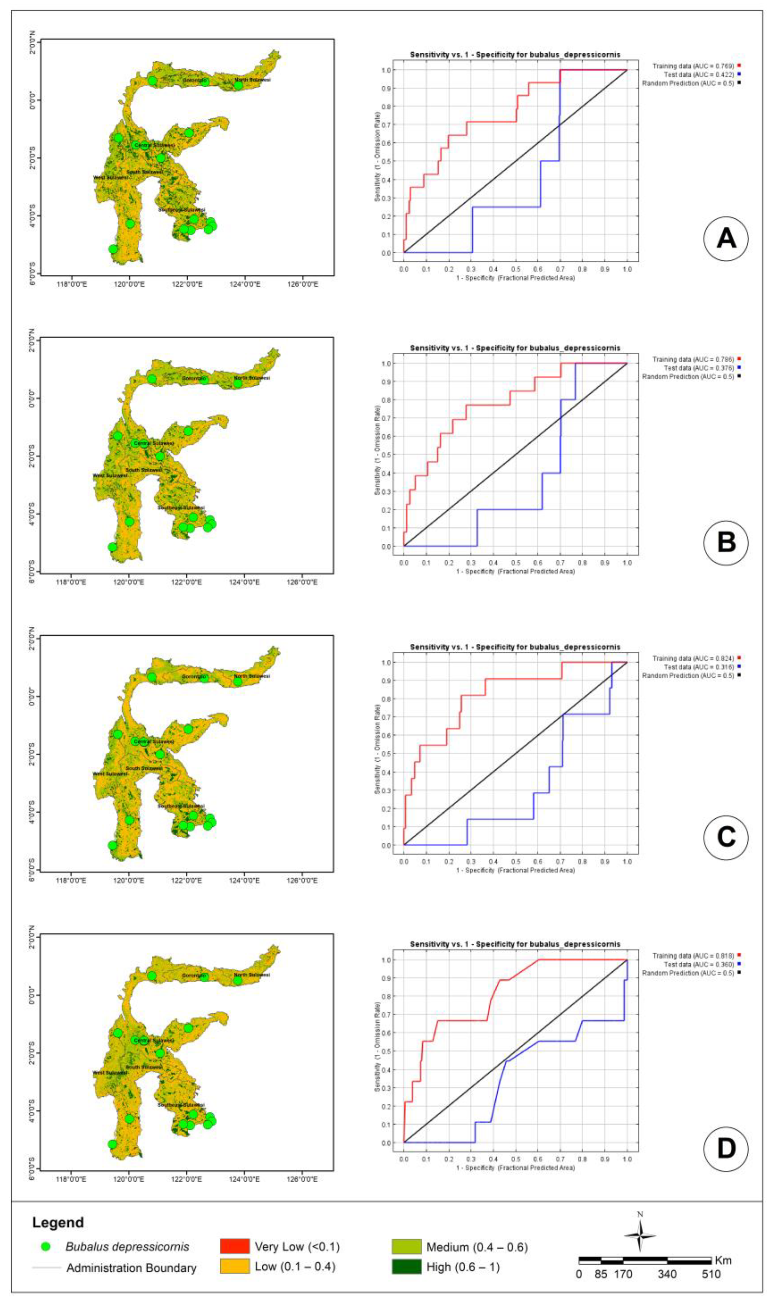
3.1. MaxEnt Modeling Results

As shown in Figure 4. Experiments were carried out to get the best results by comparing the splitting ratio of training and testing datasets, i.e., 75:25, 70:30, 60:40 and 50:50.
In the case of this MaxEnt model, the best AUC result for Bubalus quarlesi is shown as 0.947 in Figure 4 with a training and testing ratio of 60:40. This value shows good performance as it is quite close to the highest value of 1, which indicates that the MaxEnt model at a training-testing ratio of 60:40 has a reasonably good ability to distinguish the potential habitat classes of Mountain Anoa (Bubalus quarlesi).
In the case of this MaxEnt model, the best AUC result for Bubalus depressicornis was shown as 0.824 in Figure 5 with a training and testing ratio of 60:40. This value shows good performance as it is quite close to the highest value of 1, which indicates that the MaxEnt model at a training-testing ratio of 60:40 has a reasonably good ability to distinguish the potential habitat classes of Lowland Anoa (Bubalus depressicornis).

3.2. RF Modeling Results

There are four class divisions for habitat suitability modeling as shown in Figure 6.
In the case of this RF model, the best AUC result for Bubalus quarlesi was shown as 0.987 in Figure 6 with a training and testing ratio of 75:25. This value shows good performance as it is quite close to the highest value of 1, which indicates that the RF model at a training-testing ratio of 75:25 has a reasonably good ability to distinguish the potential habitat classes of Mountain Anoa (Bubalus quarlesi).
In the case of this RF model, the best AUC result for Bubalus depressicornis is shown as 0.967 in Figure 7 with a training and testing ratio of 70:30. This value shows good performance as it is quite close to the highest value of 1, which indicates that the RF model at a training-testing ratio of 70:30 has a reasonably good ability to distinguish the potential habitat classes of Lowland Anoa (Bubalus depressicornis).

3.3. Best Results

Based on the modeling results, the RF model with a training and testing ratio of 75:25 was the best algorithm for the Mountain Anoa habitat potential model with a high potential habitat area of 837,400 ha (5% of the island of Sulawesi) in Table 3 showing the results of the area of potential habitat according to its classification in each province. While for the AUC value of 0.987; Accuracy 0.975; Kappa 0.992; Sensitivity 0.944; Specificity 1; and Detection Rate 0.425.
Meanwhile, the best model for Lowland Anoa habitat potential was the RF algorithm with a training and testing ratio of 70:30 with a high potential area of 6,015,700 ha (36% of the island of Sulawesi). Table 4 shows the results of the area of potential habitat according to its classification in each province. While for the AUC value of 0.967; Accuracy 0.909; Kappa 0.814; Sensitivity 0.8; Specificity 1; and Detection Rate 0.364.
The percentage of environmental variables that support the modeling of potential habitat for Mountain Anoa (Bubalus quarlesi) and Lowland Anoa (Bubalus depressicornis) is shown in Figure 8.
Based on the graph in Figure 8a, the parameter or variable with the highest relative contribution to the Mountain Anoa habitat potential model is humidity, with a value of 82.444%. This correlates with Table 2, which shows the humidity variable to be a variable that is strongly associated with several other variables. Meanwhile, the parameter with the lowest relative contribution is the distance of the water source, with a value of 13.340%. Based on the graph in Figure 8b, the parameter or variable with the highest relative contribution to the Lowland Anoa habitat potential model is a human population with a value of 88.891%. Meanwhile, the parameter with the lowest relative contribution is land use, with a value of 6.084%.
Figure 9 illustrates the histogram of each environmental parameter used for the Mountain Anoa (Bubalus quarlesi) training point extraction. It is known that the habitat characteristics of Mountain Anoa in terms of elevation are mostly in class 5 (>2500 m above sea level). When viewed from the land cover histogram, most are in class 10 (trees), indicating that Mountain Anoa prefer to live in forest areas. Regarding vegetation index, Mountain Anoa prefer areas with a high vegetation index, namely class 4 (0.5–0.75). Mountain Anoa also prefer areas that tend to be cold or in temperature class 1 (<20 °C). Water distance tends to be in areas close to water sources (rivers and lakes), in class 1 (0–500 m). Meanwhile, the humidity is in the range of 11–13%. From the disturbance factor, the farther away from the road or transportation the Mountain Anoa can live is directly proportional to the human population factor.
Figure 10 illustrates the histogram of each environmental parameter used to extract Lowland Anoa (Bubalus depressicornis) training points. It is known that the habitat characteristics of Lowland Anoa in terms of elevation are mostly in class 1 (0–1000 masl). When viewed from the land cover histogram, most are in class 10 (trees), indicating that Lowland Anoa prefer to live in forest areas. In terms of vegetation index, Lowland Anoa prefer areas with a very high vegetation index, namely class 6 (0.75–1). Lowland Anoa also prefer areas that tend to be moderate or in temperature class 2 (20–25 °C). Water distance tends to be in areas close to water sources (rivers and lakes), in class 1 (0–500 m). Meanwhile, the humidity is in the range of 17–18%. From the disturbance factor, the farther away from the road or transportation the Mountain Anoa can live is directly proportional to the human population factor.

4. Discussion

The modeling of the habitat potential of Mountain Anoa (Bubalus quarlesi) and Lowland Anoa (Bubalus depressicornis) is supported using eight environmental variables, namely Elevation, Temperature, Vegetation, Land Cover, Transportation, Water Distance, Humidity and Human Population. The highest variable contribution for the Mountain Anoa habitat potential model is humidity with a value of 82.444% while the highest variable contribution result for the Lowland Anoa habitat potential model is human population with a value of 88.891%.
Comparisons of RF and MaxEnt methods have their own characteristics that depend on the research case. The RF method has been widely applied in the classification of remote sensing image data due to its insensitivity to noise and excessive training data and its good performance [28]. Prediction results from RF are obtained through the most results from each individual decision tree (voting for classification and averaging for regression). Because RF is the result of the most votes from each decision tree, it will issue more accurate predictions and results. This is because the more decision trees used to vote, the more accurate the resulting data will be. The principle of MaxEnt is to find the probability distribution of maximum entropy subject to a set of constraints derived from the species’ occurrence data [11].
Based on this research, the RF method is better than the MaxEnt method. This is based on the AUC value, which is used as a general evaluation metric to measure the performance of classification models. AUC reflects the model’s ability to distinguish between two different classes or categories [29]. AUC is theoretically and empirically proven to be better than accuracy metrics for evaluating classifier performance and distinguishing optimal solutions during classification training [30]. In the results of the Bubalus quarlesi habitat potential model, the RF results with a splitting ratio of training-testing 75:25 are the best results with an AUC value of 0.987. While in the results of the Bubalus depressicornis habitat potential model, the RF results with a splitting ratio training-testing 70:30 are the best results with an AUC value of 0.967. This is supported by research conducted by Zhao that the comparison of methods used in amphibian prediction in China resulted in the RF method being slightly better than the MaxEnt method. From Zhao’s research, RF may be more applicable in predicting the native potential distribution of species with sufficient species occurrence data, given the additional predictive detail, the simplicity of use, the computational time involved and operational complexity. However, another study by Kaky [31] suggests that, if an area only has a presence data format, then in that situation MaxEnt is a better choice than a complex and computationally intensive “black box” ensemble. MaxEnt can promote practical conservation goals more effectively. This means that the accuracy of predictions is influenced by several environmental variables as well as the characteristics of the case study used, so not all modeling performed shows that RF is better than other methods.

5. Conclusions

The results of the comparison of MaxEnt and RF machine learning algorithms for the potential habitat showed that the RF 75:25 model is the best algorithm for modeling Mountain Anoa habitat potential with a high habitat potential level of 837,400 ha (5% of the island of Sulawesi), with AUC values of 0.987; acc 0.975; kappa 0.992; SN 0.944; SP 1; and DR 0.425. Meanwhile, the best model for Lowland Anoa habitat potential is the RF 70:30 algorithm with a high potential area of 6,015,700 ha (36% of the island of Sulawesi), for an AUC value of 0.967; ACC 0.909; kappa 0.814; SN 0.8; SP 1; and DR 0.364. The human population parameter has the highest relative contribution rate of 89% of the model. This indicates that Anoa extinction is very sensitive to the presence of a human population and is directly proportional to the lack of potential habitat. Information from the habitat modeling study of Mountain Anoa and Lowland Anoa can be used by IUCN in community or NGO collaboration efforts and advocacy for the conservation of vulnerable animals.

Author Contributions

Conceptualization, L.M.J. and D.A.; in-situ data, S.A.; methodology, L.M.J. and D.A.; formal analysis, L.M.J. and D.A.; writing—original draft preparation, D.A.; writing—review and editing, L.M.J., M.P.T., M.I. and A.A.W.; visualization, D.A.; supervision, L.M.J., M.P.T. and M.I. All authors have read and agreed to the published version of the manuscript.

Funding

This research was funded by Institut Teknologi Sepuluh Nopember, grant number 1334/PKS/ITS/2021.

Data Availability Statement

Shuttle Radar Topography Mission (DEM) data courtesy of the U.S. National Aeronautics and Space Administration; MODIS (LST and NDVI) data courtesy of the U.S. Geological Survey; ESA WorldCover; Human Population WorldPop, Relative Humidity FLDAS: Famine Early Warning Systems Network (FEWS NET) Land Data Assimilation System; Road, Lake, and Rivers (Waters) data courtesy of the Indonesia Information Geospatial Agency.

Acknowledgments

The author would like to thank the collaborative research team from University of Indonesia, University of West Sulawesi, IPB University and Insitut Teknologi Sepuluh Nopember who have helped provide facilities for supporting in-situ data in this research.

Conflicts of Interest

The authors declare no conflict of interest.

Appendix A

Table A1. In-situ data on the coordinates of Anoa tracks.
NoSpesiesLongitude (°)Latitude (°)Source
1Bubalus quarlesi120.51870−1.57008[32]
2Bubalus quarlesi120.04250−0.80722[33]
3Bubalus quarlesi120.04050−0.81842[33]
4Bubalus quarlesi120.04510−0.80831[33]
5Bubalus quarlesi120.21340−1.52712[34]
6Bubalus quarlesi120.00920−1.68975[34]
7Bubalus quarlesi123.809600.47658[35]
8Bubalus quarlesi123.809900.46652[35]
9Bubalus quarlesi121.005700.60439[36]
10Bubalus quarlesi120.00180−0.82303[37]
11Bubalus quarlesi120.01500−0.80661[37]
12Bubalus quarlesi120.03370−0.83094[37]
13Bubalus quarlesi120.01270−0.82683[37]
14Bubalus quarlesi120.77800−2.20443[38]
15Bubalus quarlesi120.96800−1.69737[38]
16Bubalus quarlesi120.97300−2.39240[38]
17Bubalus quarlesi119.87400−3.07609[38]
18Bubalus quarlesi119.39188−2.87850-
19Bubalus quarlesi119.39369−2.87648Footprints
20Bubalus quarlesi119.39366−2.87647Resting Place
21Bubalus quarlesi119.39366−2.87646Footprints
22Bubalus quarlesi119.39450−2.873132 Year Old Juvenile Female Stool—1 Week Stool Age—11 cm × 10 cm
23Bubalus quarlesi119.38334−2.87160Traces—1 Month—3 Years Old
24Bubalus quarlesi119.38450−2.86527Parent Footprints—1 Week—5.5 cm × 6.5 cm
25Bubalus quarlesi119.38459−2.86526Child’s Footprints—1 Week—3 cm × 3.5 cm
26Bubalus quarlesi119.38456−2.85850Male Stool—1 Week Stool Age
27Bubalus quarlesi119.38484−2.842803 Day Trail 6 × 7—1.5 cm deep
28Bubalus quarlesi119.38478−2.842753 Month Old Stool—13.5 × 14
29Bubalus quarlesi119.38467−2.842978 Month Anoa Trail—4.5 × 5.5
30Bubalus quarlesi119.38460−2.84316Male Stool—1 Week Old—20.5 × 3
31Bubalus quarlesi119.38274−2.84330Anoa Trail 1 Week—6 × 8. 1.4 cm deep
32Bubalus quarlesi119.38276−2.843313-Month Male Stool—26 × 13.5
33Bubalus quarlesi119.38274−2.84322Nest 82 cm × 41 cm
34Bubalus quarlesi119.38277−2.84351-
35Bubalus quarlesi119.38277−2.84351Male Trail—7 Years Old—3 Day Trail—7.4 cm × 7 cm—2 cm Depth
36Bubalus quarlesi119.38276−2.843517 Year Old Female Trail—3 Day Trail—4 cm × 7 cm—1.5 cm Depth
37Bubalus quarlesi119.38561−2.843615 Day Trail—6 × 8—2 cm deep
38Bubalus quarlesi119.38596−2.843502 Day Trail—5.3 cm × 8 cm—2 cm Depth
39Bubalus quarlesi119.38623−2.84363Resting Place—90 cm × 80 cm × 40 cm
40Bubalus quarlesi119.38655−2.84368Juvenile Stool < 1 Year—1 Week Stool Age—6.5 cm × 7.5 cm
41Bubalus quarlesi119.38652−2.84372Child Trail (Youth)—1 Week Trail Age—4 cm × 5.7 cm
42Bubalus quarlesi119.38697−2.84411Footprints of 5 Year Old Male—Age of Footprints 2 Days—6 cm × 7 cm—Depth 0.9 cm—Blunt Hooves
43Bubalus quarlesi119.38616−2.84435Male Stool—1 Month Stool Age—9.5 cm × 10 cm
44Bubalus quarlesi119.38577−2.84400Female Trail 4–5 Years—Trail Age 8 Days—6.5 cm × 7.5 cm—Depth 1 cm
45Bubalus quarlesi119.38574−2.843974–5 Year Old Female Manure—2 Weeks Manure Age—20.5 cm × 23.5 cm
46Bubalus quarlesi119.38575−2.843862.5 Year Old Male Trail—3 Day Trail Age—6.6 cm × 4.5 cm—2 cm Depth
47Bubalus quarlesi119.38567−2.84387Female Resting Place—90 cm × 60 cm × 35 cm
48Bubalus quarlesi119.38565−2.84387Female Trail—2 Weeks of Trail Age—6 cm × 7 cm—1 cm Depth
49Bubalus quarlesi119.38482−2.844011.5 Year Old Male Imprint—3 Weeks Manure Age—10.5 cm × 10 cm
50Bubalus quarlesi119.38482−2.843861.5 Year Old Male Trail—3 Week Trail—5 cm × 6.5 cm—2 cm Depth
51Bubalus quarlesi119.38323−2.84537Footprint—6 cm × 7.5 cm—2.3 cm depth
52Bubalus quarlesi119.38309−2.84509Footprint—5.3 cm × 8 cm—3 cm depth
53Bubalus quarlesi119.38311−2.84484Stools—16 cm × 10 cm
54Bubalus quarlesi119.38872−2.842014 Day Female Trail—5 cm × 7 cm—1.4 cm Depth
55Bubalus quarlesi119.38878−2.841944 Day Male Trail—7 cm × 6 cm—1.5 cm depth
56Bubalus quarlesi119.39028−2.83982Lantalomo Peak
57Bubalus quarlesi119.39047−2.838733 Month Male Manure—9 cm × 12 cm
58Bubalus quarlesi119.39124−2.837103 Day Female Trail—6 cm × 6 cm—1 cm depth
59Bubalus quarlesi119.39193−2.835861 Month Female Manure—14 cm × 12 cm
60Bubalus quarlesi119.39194−2.835841.5 Year Old Child Imprint—2 Weeks Imprint Age—3 cm × 5 cm—Depth
61Bubalus quarlesi119.39316−2.832152 Day Female Trail—6 cm × 8 cm—3 cm depth
62Bubalus quarlesi119.39316−2.83197Female footprint 2–3 yrs—1 week footprint—6 cm × 8 cm—2 cm deep
63Bubalus quarlesi119.39289−2.824192 Day Female Trail—6 cm × 6 cm—2 cm depth
64Bubalus quarlesi119.38518−2.82199The Nest
65Bubalus quarlesi119.38431−2.82164Stools—18 cm × 20 cm
66Bubalus quarlesi119.38346−2.81992Stools—14 cm × 15 cm
67Bubalus quarlesi119.38342−2.81958Stools—16 cm × 13 cm
68Bubalus quarlesi119.38349−2.81960Male Manure 1 Day—9 cm × 8 cm
69Bubalus quarlesi119.38172−2.81800Female Manure < 1 Year Old—1 Week Manure—12 cm × 14 cm
70Bubalus quarlesi119.38175−2.818022 Month Old imprint—8 cm × 9 cm—3 cm depth
71Bubalus quarlesi119.38089−2.81808Male Tracks Age > 1 Year—3 Day Tracks—5 cm × 6.5 cm—2 cm depth
72Bubalus quarlesi119.38098−2.818045–6 Year Old Female Stool—5 Day Stool—29.5 cm × 18 cm
73Bubalus quarlesi119.38108−2.817911 Day Female Trail—6.3 cm × 7 cm—0.6 cm Depth
74Bubalus quarlesi119.38101−2.817921 Day Male Footprint—4.5 cm x 5 cm—1 cm depth
75Bubalus quarlesi119.37827−2.816874 Day Female Trail—4.5 cm × 8 cm—1 cm depth
76Bubalus quarlesi119.37728−2.81484Nest—95 cm × 113 cm × 64 cm
77Bubalus quarlesi119.37725−2.81487Resting Place
78Bubalus quarlesi119.37707−2.815251 Day Female Trail—6 cm × 9 cm—1 cm depth
79Bubalus quarlesi119.37729−2.81541Male Footprints 1 Day—5.5 cm x 6.3 cm—0.5 cm Depth
80Bubalus quarlesi119.37739−2.815381 Week Female Manure—15.5 cm × 14 cm
81Bubalus quarlesi119.37747−2.815562 Year Old Male Stool—1 Day Stool Age—13.7 cm × 9 cm
82Bubalus quarlesi119.37746−2.81560Female Trail 4–5 years old—Trail Age 1 Day—5.1 cm × 7 cm—Depth 3 cm
83Bubalus quarlesi119.38848−2.823641.5 Year Male Stool—1 Day Stool Age—10 cm × 8 cm
84Bubalus quarlesi119.39298−2.82827Parent male 1.5 years old—1 day old—4.5 cm × 6 cm—0.3 cm depth
85Bubalus depressicornis122.12180−4.49525[39]
86Bubalus depressicornis120.52510−1.58031[32]
87Bubalus depressicornis120.52360−1.57728[32]
88Bubalus depressicornis120.51810−1.56668[32]
89Bubalus depressicornis123.768000.51531[38]
90Bubalus depressicornis122.610000.62516[38]
91Bubalus depressicornis120.21500−1.55003[38]
92Bubalus depressicornis120.793000.66886[38]
93Bubalus depressicornis119.61900−1.30254[38]
94Bubalus depressicornis122.06100−1.13299[38]
95Bubalus depressicornis121.87800−4.45523[38]
96Bubalus depressicornis122.80600−4.20800[38]
97Bubalus depressicornis122.87000−4.35533[38]
98Bubalus depressicornis122.72800−4.47538[38]
99Bubalus depressicornis119.43333−5.15000[40]
100Bubalus depressicornis120.02000−4.27083[40]
101Bubalus depressicornis121.08086−2.00000[40]
102Bubalus depressicornis122.23148−4.11590[40]

References

  1. Mustari, A.H. Ekologi, Perilaku, dan Konservasi Anoa (Ecology, Behaviour, and Conservation of Anoa, Bovidae: Bubalus depressicornis and Bubalus quarlesi); Bogor, C.P., Ed.; PT Penerbit IPB Press: Bogor City, Indonesia, 2019. [Google Scholar]
  2. IUCN. The 2013 IUCN Red List of Threatened. 2013. Available online: https://www.iucnredlist.org/ (accessed on 13 September 2021).
  3. Groves, C.P. Systematics of the Anoa (Mammalia, Bovidae). Zool. Museum Univ. Amst. 1969, 17, 1–12. [Google Scholar]
  4. Harper, F. Extinct and Vanishing Mammals of the Old World; American Committee for International Wild Life Protection: New York, NY, USA, 1945; Available online: https://www.biodiversitylibrary.org/item/59320 (accessed on 5 January 2022).
  5. Fradrich, H. Einige Bemerkungen Uber den Anoa; Zeitschrift des Kolner Zoo: Bakersfield, CA, USA, 1973; Volume 16. [Google Scholar]
  6. Ardiani, D.; Jaelani, L.M.; Aldiansyah, S.; Tambunan, M.P.; Indrawan, M.; Wibowo, A.A. The Effect of Human Disturbance on the Spatial Distribution of Anoa (Bubalus sp.) Using MaxEnt Modeling. IOP Conf. Ser. Earth Environ. Sci. 2023, 1127, 012020. [Google Scholar] [CrossRef]
  7. Jaelani, L.M.; Benedict; Ardiani, D.; Tambunan, M.P.; Indrawan, M.; Wibowo, A.A. An Extensive Coverage Anoa Distribution Modelling in Sulawesi Using Maximum Entropy. HAYATI J. Biosci. 2023, 30, 716–724. [Google Scholar] [CrossRef]
  8. Zhao, Z.; Xiao, N.; Shen, M.; Li, J. Comparison Between Optimized MaxEnt and Random Forest Modeling in Predicting Potential Distribution: A Case Study with Quasipaa boulengeri in China. Sci. Total Environ. 2022, 842, 156867. [Google Scholar] [CrossRef] [PubMed]
  9. Ao, Y.; Li, H.; Zhu, L.; Ali, S.; Yang, Z. The linear random forest algorithm and its advantages in machine learning assisted logging regression modeling. J. Pet. Sci. Eng. 2019, 174, 776–789. [Google Scholar] [CrossRef]
  10. Fawagreh, K.; Gaber, M.M.; Elyan, E. Random forests: From early developments to recent advancements. Syst. Sci. Control Eng. 2014, 2, 602–609. [Google Scholar] [CrossRef]
  11. Phillips, S.J.; Anderson, R.P.; Schapire, R.E. Maximum Entropy Modeling of Species Geographic Distributions. Int. J. Glob. Environ. Issues 2006, 6, 231–259. [Google Scholar] [CrossRef]
  12. Nurwatik, N.; Ummah, M.H.; Cahyono, A.B.; Darminto, M.R.; Hong, J.H. A Comparison Study of Landslide Susceptibility Spatial Modeling Using Machine Learning. ISPRS Int. J. Geo-Inf. 2022, 11, 602. [Google Scholar] [CrossRef]
  13. Pemerintah Pusat, UU Nomor 5 Tahun 1994. 1994. Available online: https://peraturan.go.id/id/uu-no-5-tahun-1994 (accessed on 5 January 2022).
  14. Sosilowati, S.T.; Handayani, A.; Wahyudi, A.R.; Massudi, W.; Febrianto, S.; Suhendri, N.A. Sinkronisasi Program dan Pembiayaan Pembangunan Jangka Pendek 2018–2020; PUPR: San Juan, PR, USA, 2017. [Google Scholar]
  15. USGS. Earth Explorer. 2022. Available online: https://earthexplorer.usgs.gov/ (accessed on 5 September 2022).
  16. Phillips, S.J.; Dudík, M.; Schapire, R.E. Maxent Software for Modeling Species Niches and Distributions (Version 3.4.1). 2021. Available online: http://biodiversityinformatics.amnh.org/open_source/maxent/ (accessed on 1 September 2021).
  17. Chambers, J.M. The Comprehensive R Archive Network. 2021. Available online: https://cran.r-project.org/ (accessed on 1 November 2021).
  18. GEE. Google Earth Engine. 2022. Available online: https://code.earthengine.google.com/ (accessed on 11 July 2022).
  19. Baldwin, R.A. Use of maximum entropy modeling in wildlife research. Entropy 2009, 11, 854–866. [Google Scholar] [CrossRef]
  20. Phillips, S. ‘A Brief Tutorial on Maxent’ in Species Distribution Modeling for Educators and Practitioners. Lessons Conserv. 2010, 3, 107–135. Available online: http://ncep.amnh.org/linc (accessed on 3 September 2021).
  21. Kumar, S.; Stohlgren, T.J. Maxent modeling for predicting suitable habitat for threatened and endangered tree Canacomyrica monticola in New Caledonia. J. Ecol. Nat. Environ. 2009, 1, 94–98. [Google Scholar]
  22. Noer, I.S.; Gunawan, H.; Rahman, D.A. Penggunaan Habitat dan Pemodelan Distribusi Spasial Macan Tutul Jawa di Kawasan Gunung Sawal Jawa Barat. J. Penelit. Hutan Dan Konserv. Alam 2021, 18, 53–66. [Google Scholar] [CrossRef]
  23. Li, Z.; Liu, Y.; Zeng, H. Application of the MaxEnt model in improving the accuracy of ecological red line identification: A case study of Zhanjiang, China. Ecol. Indic. 2022, 137, 108767. [Google Scholar] [CrossRef]
  24. West, A.M.; Kumar, S.; Brown, C.S.; Stohlgren, T.J.; Bromberg, J. Field validation of an invasive species Maxent model. Ecol. Inform. 2016, 36, 126–134. [Google Scholar] [CrossRef]
  25. Gorunescu, F. Data Mining Concepts, Models and Techniques; Springer: Berlin/Heidelberg, Germany, 2011. [Google Scholar] [CrossRef]
  26. Chicco, D.; Warrens, M.J.; Jurman, G. The Matthews Correlation Coefficient (MCC) is More Informative Than Cohen’s Kappa and Brier Score in Binary Classification Assessment. IEEE Access 2021, 9, 78368–78381. [Google Scholar] [CrossRef]
  27. Petrosino, A.; Salvi, G. A Rough Fuzzy Neural Network Approach for Robust Face Detection and Tracking; Elsevier Inc.: Amsterdam, The Netherlands, 2015. [Google Scholar] [CrossRef]
  28. Yang, S.; Berdine, G. The receiver operating characteristic (ROC) curve. Southwest Respir. Crit. Care Chron. 2017, 5, 34. [Google Scholar] [CrossRef]
  29. Narkhede, S. Understanding AUC–ROC Curve. Towar. Data Sci. 2018, 6–11. Available online: https://towardsdatascience.com/understanding-auc-roc-curve-68b2303cc9c5 (accessed on 13 June 2023).
  30. Trifonova, O.P.; Lokhov, P.G.; Archakov, A.I. Metabolic profiling of human blood. Biochem. Suppl. Ser. B Biomed. Chem. 2013, 7, 179–186. [Google Scholar] [CrossRef]
  31. Kaky, E.; Nolan, V.; Alatawi, A.; Gilbert, F. A comparison between Ensemble and MaxEnt species distribution modelling approaches for conservation: A case study with Egyptian medicinal plants. Ecol. Inform. 2020, 60, 101150. [Google Scholar] [CrossRef]
  32. Ranuntu, R.A.; Mallombasang, S.N. Studi Populasi dan Habitat Anoa (Bubalus sp.) si Kawasan Hutan Lindung Desa Sangginora Kabupaten Poso. Mitra Sains 2015, 3, 81–94. [Google Scholar]
  33. Wardah, W.; Labiro, E.; Massiri, S.D.; Sustri, S.; Mursidin, M. Vegetasi Kunci Habitat Anoa Di Cagar Alam Pangi Binangga, Sulawesi Tengah. J. Penelit. Kehutan. Wallacea 2012, 1, 1–12. [Google Scholar] [CrossRef]
  34. Stephens, W. Anoa Gunung (Bubalus quarlesi). 2014. Available online: https://www.inaturalist.org/observations/40653991 (accessed on 3 September 2021).
  35. Arini, D.I.D. Anoa dan Habitatnya di Sulawesi Utara; no. 1; Balai Penelitian Kehutanan Manado: Manado, Indonesia, 2013.
  36. Allo, R.P.A.; Sudhartono, A.; Labiro, E. Karakteristik Komponen Abiotik Anoa (Bubalus sp.) Habitat dalam Hutan Pendidikan Tadulako Universitas Kecamatan Bolano Lambunu Kabupaten Parigi Moutong. J. War. Rimba 2018, 6, 25–31. [Google Scholar]
  37. Valentino, M.W.S. Distribusi Jejak Anoa (Bubalus sp.) di Kawasan Cagar Alam Pangi Binangga Kabupaten Parigi Moutong. 2013. Available online: https://dokumen.tips/documents/distribusi-jejak-anoa-bubalus-spp-di-kawasan-cagar-alam-pangi-binangga-kab.html?page=1 (accessed on 17 September 2023).
  38. Burton, J.A. The taxonomic status, distribution and conservation of the lowland anoa Bubalus depressicornis and mountain anoa Bubalus quarlesi. Mamm. Rev. 2005, 35, 25–50. [Google Scholar] [CrossRef]
  39. Analuddin, K.; Raya, R.; Rahim, S. Struktur Hutan Mangrove Sebagai Habitat Hewan Endemik Anoa Dataran Rendah (Bubalus sp.) di Taman Nasional Rawa Aopa Watumohai. BioWallacea J. Biol. Res. 2016, 3, 384–395. [Google Scholar]
  40. GBIF. Occurrence Download; The Global Biodiversity Information Facility: Copenhagen, Denmark, 2023. [Google Scholar] [CrossRef]
Figure 1. Research area: (a) Sulawesi Island, (b) location of Sulawesi Island on Indonesia Map, (c) location of Indonesia on the World Map.
World 04 00041 g001
Figure 2. Processing flow-chart.
World 04 00041 g002
Figure 3. Environmental variables for predicting the potential of Anoa habitat.
World 04 00041 g003
Figure 4. Map (left) and ROC/AUC curve (right) of the Bubalus quarlesi habitat potential model with MaxEnt algorithm (training-test ratio in %, (A) 75:25, (B) 70:30, (C) 60:40, (D) 50:50).
World 04 00041 g004
Figure 5. Map and ROC/AUC curve of the Bubalus depressicornis habitat potential model with MaxEnt algorithm (training-test ratio in %, (A) 75:25, (B) 70:30, (C) 60:40, (D) 50:50).
World 04 00041 g005
Figure 6. Map and ROC/AUC curve of the Bubalus quarlesi habitat potential model with RF algorithm (training-test ratio in %, (A) 75:25, (B) 70:30, (C) 60:40, (D) 50:50).
World 04 00041 g006
Figure 7. Map and ROC/AUC curve of the Bubalus depressicornis habitat potential model with RF algorithm (training-test ratio in %, (A) 75:25, (B) 70:30, (C) 60:40, (D) 50:50).
World 04 00041 g007
Figure 8. Contribution Variables in RF Modeling (a) Bubalus quarlesi 75:25, (b) Bubalus depressicornis 70:30.
World 04 00041 g008
Figure 9. Histogram of training point parameters of Mountain Anoa (Bubalus quarlesi).
World 04 00041 g009
Figure 10. Histogram of training point parameters of Lowland Anoa (Bubalus depressicornis).
World 04 00041 g010
Table 1. Environmental variables used in the MaxEnt and RF models.
NoVariablesCell Size (m)SourceClassRange Data
1DEM/Elevation30Shuttle Radar Topography Mission (SRTM)10–1000 m
21000–1500 m
31500–2000 m
42000–2500 m
5>2500 m
2Temperature100 (resampled to 30)MOD11A1 Version 6 product1<20 °C
220–25 °C
325–30 °C
4>30 °C
3Vegetation Index100 (resampled to 30)MOD11A1 Version 6 product1<0
20–0.25
30.25–0.50
40.50–0.75
50.75–1
4Land Cover10 (resampled to 30)ESA WorldCover10Trees
20Shrubland
30Grassland
40Cropland
50Built-up
60Barren/Sparse Vegetation
80Open Water
90Herbaceous Wetland
95Mangroves
5Transportation30BIG10–500 m
2501–1000 m
31001–1500 m
41501–2000 m
5>2000 m
6Water30BIG10–500 m
2501–1000 m
31001–1500 m
41501–2000 m
5>2000 m
7Human Population100 (resampled to 30)WorldPop0–1553 people/pixel
8Relative Humidity11,000 (resampled to 30)FLDAS9.45–19.34%
Table 2. Correlation between variables.
ElevationTemperatureVegetationRelative HumidityHuman PopulationLand CoverWaterTransportation
Elevation1
Temperature−0.8511
Vegetation−0.6720.4781
Relative Humidity−0.9120.9320.5131
Human Population−0.1590.345−0.2550.2181
Land Cover−0.2370.4030.0380.3530.4601
Water−0.5010.4820.3790.5410.051−0.0431
Transportation0.467−0.666−0.260−0.549−0.367−0.272−0.3161
Table 3. Potential Bubalus quarlesi habitat area in each province on Sulawesi Island (in hectares).
ProvinceGorontaloWest SulawesiSouth SulawesiCentral SulawesiSoutheast SulawesiNorth Sulawesi
Class
Very Low676,577784,3212,247,5742,283,9171,337,869666,963
Low473,689624,6901,602,2932,719,1511,164,064496,856
Medium17,70593,083227,439329,48075,10525,420
High20,383129,326285,650295,18471,25635,613
Table 4. Potential Bubalus depressicornis habitat area in each province on Sulawesi Island (in hectares).
ProvinceGorontaloWest SulawesiSouth SulawesiCentral SulawesiSoutheast SulawesiNorth Sulawesi
Class
Very Low23,77317,105179,47691,70423,91533,029
Low317,990372,4821,638,1321,238,548638,400347,087
Medium504,452584,0041,185,0451,865,1101,144,664465,104
High342,139657,8291,360,3042,432,371841,315379,632
Disclaimer/Publisher’s Note: The statements, opinions and data contained in all publications are solely those of the individual author(s) and contributor(s) and not of MDPI and/or the editor(s). MDPI and/or the editor(s) disclaim responsibility for any injury to people or property resulting from any ideas, methods, instructions or products referred to in the content.

