
Multi-Point Shape Optimization of a Horizontal Axis Tidal Stream Turbine


Institute of Ship Technology Ocean Engineering and Transport Systems, University of Duisburg-Essen, Bismarckstrasse 69, 47057 Duisburg, Germany
*
Author to whom correspondence should be addressed.
Eng 2021, 2(3), 340-355; https://0-doi-org.brum.beds.ac.uk/10.3390/eng2030022
Submission received: 9 July 2021
/
Revised: 22 August 2021
/
Accepted: 24 August 2021
/
Published: 30 August 2021
(This article belongs to the Special Issue Feature Papers in Eng)
Abstract
:A method was developed to perform shape optimization of a tidal stream turbine hydrofoil using a multi-objective genetic algorithm. A bezier curve parameterized the reference hydrofoil profile NACA 63815. Shape optimization of this hydrofoil maximized its lift-to-drag ratio and minimized its pressure coefficient, thereby increasing the turbines power output power and improving its cavitation characteristics. The Elitist Non-dominated Sorting Genetic Algorithm (NSGA-II) was employed to perform the shape optimization. A comparative study of two- and three-dimensional optimizations was carried out. The effect of varying the angle of attack on the quality of optimized results was also studied. Predictions based on two-dimensional panel method results were also studied. Predictions based on a two-dimensional panel method and on a computational fluid dynamics code were compared to experimental measurements.
1. Introduction
The demand for renewable energy has been increasing over the previous decade. Renewable energy resources are available in various forms; one of them is tidal energy. Tidal energy can be harnessed in a number of ways, one being the use of tidal stream turbines. Therefore, the shape of the subject hydrofoil itself was optimized to improve the performance. The optimization process can be thought of as making the best use of resources under given constraints. Many researchers performed a two-dimensional shape optimization of airfoils for aircraft [1,2,3] and others for wind turbines [4,5]. For wind turbines, airfoils can be operated at a high angle of attack (AOA), even under stall conditions, which is not the case for aircraft. The lift-to-drag ratio (L/D) or glide ratio (GR) are the most important criteria for shape optimization of wind turbine airfoil [5]. The same methods and algorithms that optimize airfoils can be used to optimize hydrofoils. However, the parameters to be optimized differ because every turbomachine has its own optimization targets that should be taken into account. Besides the L/D ratio, cavitation characteristics should be considered to perform shape optimization of hydrofoil ([6]). Liu and Veitch [7] developed a code to predict the strength of wind turbine blades and to evaluate the maximum bald thickness. They validated their code against model and full-scale experimental measurements. Besides increasing the strength of the turbine blade, Goundar and Ahmed [8] designed hydrofoils for different sections of an HATST to maximize its L/D ratio and to reduce the possibility of the occurrence of cavitation.
Paolo et al. [9] optimized marine propeller hydrofoils by taking into account the effect of cavitation. They parameterized the hydrofoil using B-Splines [10] and carried out shape optimization using NSGA-2 [11] to widen the cavitation bucket of parent hydrofoil and to maximize L/D ratio. To this end, they employed two different flow solver approaches: viscid and inviscid. The author investigated the influence of optimization algorithms such as NSGA-2 and Particle Swarm Optimization (PSO) [12,13] on the performance of marine propeller design. Three modified optimization algorithms were proposed, two of which were based on NSGA-2 algorithm that was modified by a meta-model and one of which is non-dominated PSO algorithm that is a combination of NSGA-2 algorithm and standard PSO algorithm. Tests were carried out on a real-life propeller for naval application. The propeller geometry was described by Rolls-Royce distribution curves which can be controlled by input parameters such as blade area ratio, skew, or rake at the blade tip. Further, B-splines were used to change the geometry of the blade locally. Among the two algorithms presented that utilize a meta-model, the performance of SANA NSGA-2 was comparably better and the fastest and strictest convergence towards the Pareto front was observed in Non-dominated sorting PSO algorithm. The most important criterion for the marine propellers is to reduce the possibility of cavitation occurrence and to maximize the L/D ratio. Some researchers performed shape optimization of hydrofoils for marine applications. Ching-Yeh et al. [14] and Ouyang et al. [15] performed shape optimization for increasing the GR. Apart from GR, the authors of [16] also evaluated cavitation characteristics of the optimized hydrofoil using Computational Fluid Dynamics (CFD). Litvinov [17] optimized the shape of a hydrofoil, which moves with low velocity in a viscous incompressible fluid, to minimize the power needed to move it by imposing constraints on lift force, area, and geometry of the hydrofoil. Goundar et al. [18] studied the hydrodynamic characteristics of HF-Sx hydrofoil experimentally and numerically, and compared their performance to other hydrofoils of marine current turbines. Furthermore, they designed a hydrofoil to work well at TSRs from 3.0 to 4.0 without decreasing the possibility of cavitation. Tahani and Babayan [19] carried out shape optimization for horizontal axis turbines to increase their power coefficient by employing an Ant Colony Optimization (ACO) algorithm, and they calculated the power coefficient using Blade Element Momentum Theory (BEMT). Luo et al. [6] optimized the shape of a hydrofoil for marine current turbines to increase its L/D ratio and to improve its cavitation performance over a wide range of AOA. They parameterized the hydrofoil using Bezier curve and carried out optimization by employing NSGA-2. Furthermore, they developed a FORTRAN code and coupled it with CFD solver. The optimization method proposed in the paper effectively improves the L/D performance of the hydrofoil from AOA 0° to 12°. The cavitation performance was mainly improved from AOA 6° to 12° with little improvement from 0° to 6°.
In this paper, we carried out shape optimization of a tidal stream turbine hydrofoil to improve its output power. We developed a Matlab code to optimize the shape of its hydrofoil and coupled our code with a flow solver to determine the turbine’s performance. We chose NSGA-2 as the optimization algorithm and carried out a comparative two- and three-dimensional optimization study. One of the salient features of the NSGA-2 algorithm is that if a situation arises wherein the optimization algorithm can select only one of the two good solutions for the next generation, it makes its selection on the basis of its distance from its neighbors on the Pareto-optimal graph. The solution with the greatest distance from its neighbors is selected. This ensures that the optimized hydrofoils are diverse. Many researchers used CFD as a flow-solver, which is time-intensive. Here, we coupled our optimization code with the 2D panel, which is computationally less time-intensive and accurate. Furthermore, we investigated the effect of angle of attack on the quality of optimization results.
2. Optimization Methodology
Optimization algorithms can be categorized into two groups: gradient-based methods and heuristic algorithms. Gradient-based methods usually require derivatives of the objective functions to guide the search process. Although efficient, these methods do not always converge to global optima [5]. The convergence of the gradient-based methods depends on the initial guess. Heuristic algorithms, on the other hand, are slower, but they converge to global optima regardless of the initial guess. Objective functions alone suffice for the optimization. A Genetic Algorithm (GA) is the most popular of the heuristic algorithms. The GAs fall into two categories: single- and multi-objective GAs. For practical engineering applications, it is unrealistic to perform optimizations based on only one objective and to ignore the others.
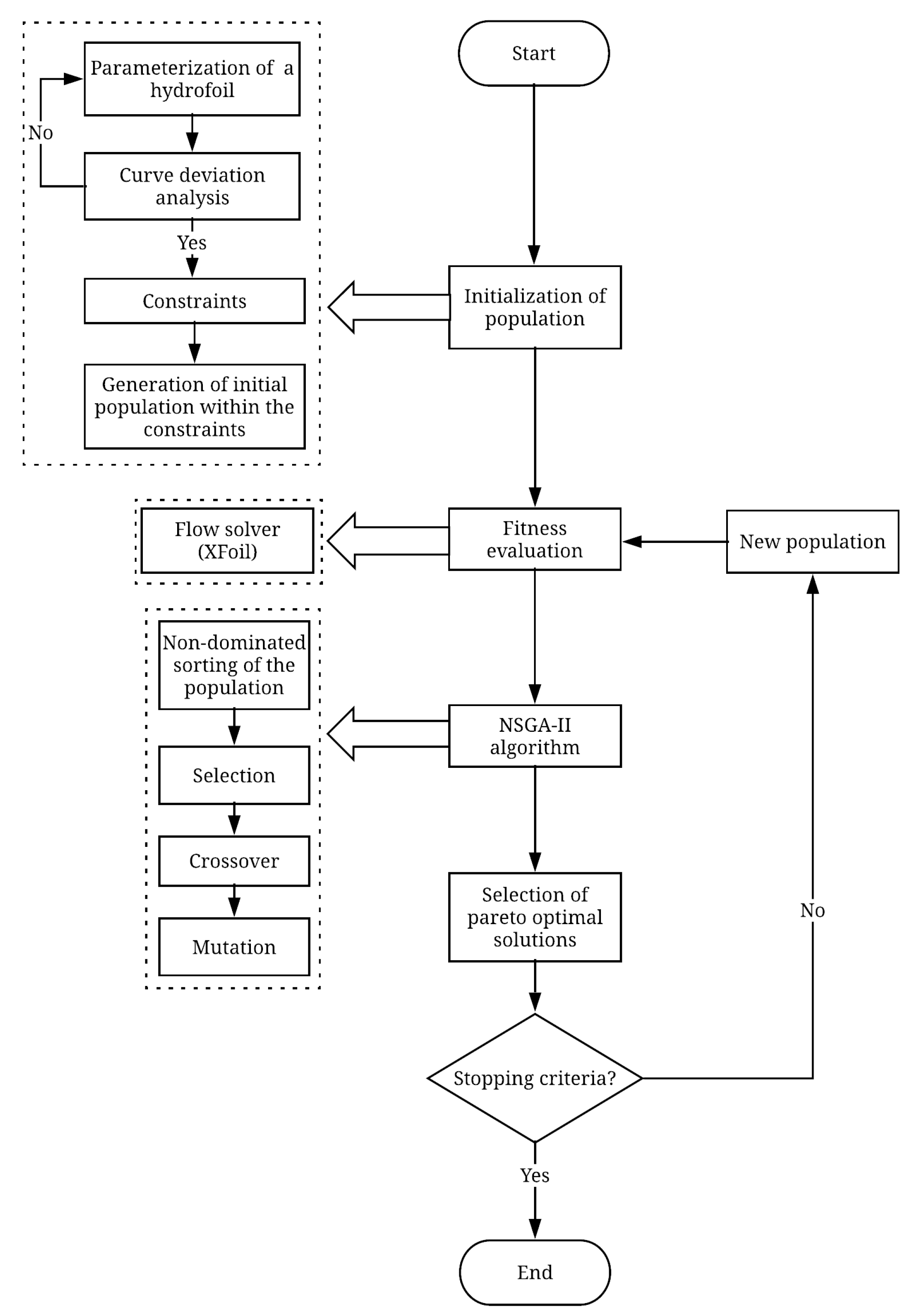
It is prudent to consider all relevant parameters [20]. The GAs are optimization techniques that solve nonlinear or non-differentiable optimization problems. They start with an initial set of randomly generated solutions, which are then compared with the objective function. Subsequent generations are generated from previous generations. We developed a new code for two- and three-dimensional shape optimizations based on the Elitist Non-dominated Sorting Genatic Algorithm (NSGA-2), using the code of [21] as the starting point. We incorporated another set of codes that parameterized the reference hydrofoil to constrain the shape of the generated hydrofoils. This limited the upper and lower bounds of the generated hydrofoils and evaluated the crowding distance for the three-dimensional optimization. Then, we modified the conditions for a non-dominating sorting of the optimized hydrofoils. Finally, we coupled this code with the flow solver and added a postprocessing library to rearrange the results to meet our requirements. Figure 1 schematically depicts our optimization method.
2.1. Initialization of Population
The initialization of population was done in three steps: parameterization of the reference hydrofoil, definition of constraints, and generation of initial population. Here, parameterization refers to the process of representing the hydrofoil shape mathematically and determining its control points, which in turn can vary and control the shape of the hydrofoils. In this study, the reference hydrofoil was parameterized using Bezier curve. A Bezier curve of order n is defined by
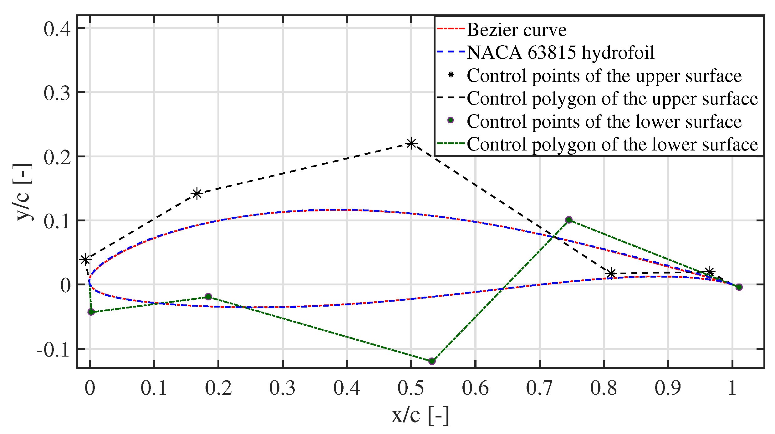
where is a point on the Bezier curve, is the weight coefficient of the point on the Bezier curve, is the Bernstein basis function, is the ith control vertex of the Bezier curve, and is the combinatorial symbol [6]. The hydrofoil NACA 63815 [22] was selected as the reference hydrofoil as it was assessed to be cavitation free through experiments [23]. In Figure 2, the original and parametrized hydrofoil are shown. It can be seen that the Bezier curve represents the hydrofoil accurately, and by moving the control points, the shape of the hydrofoil can be varied and controlled.
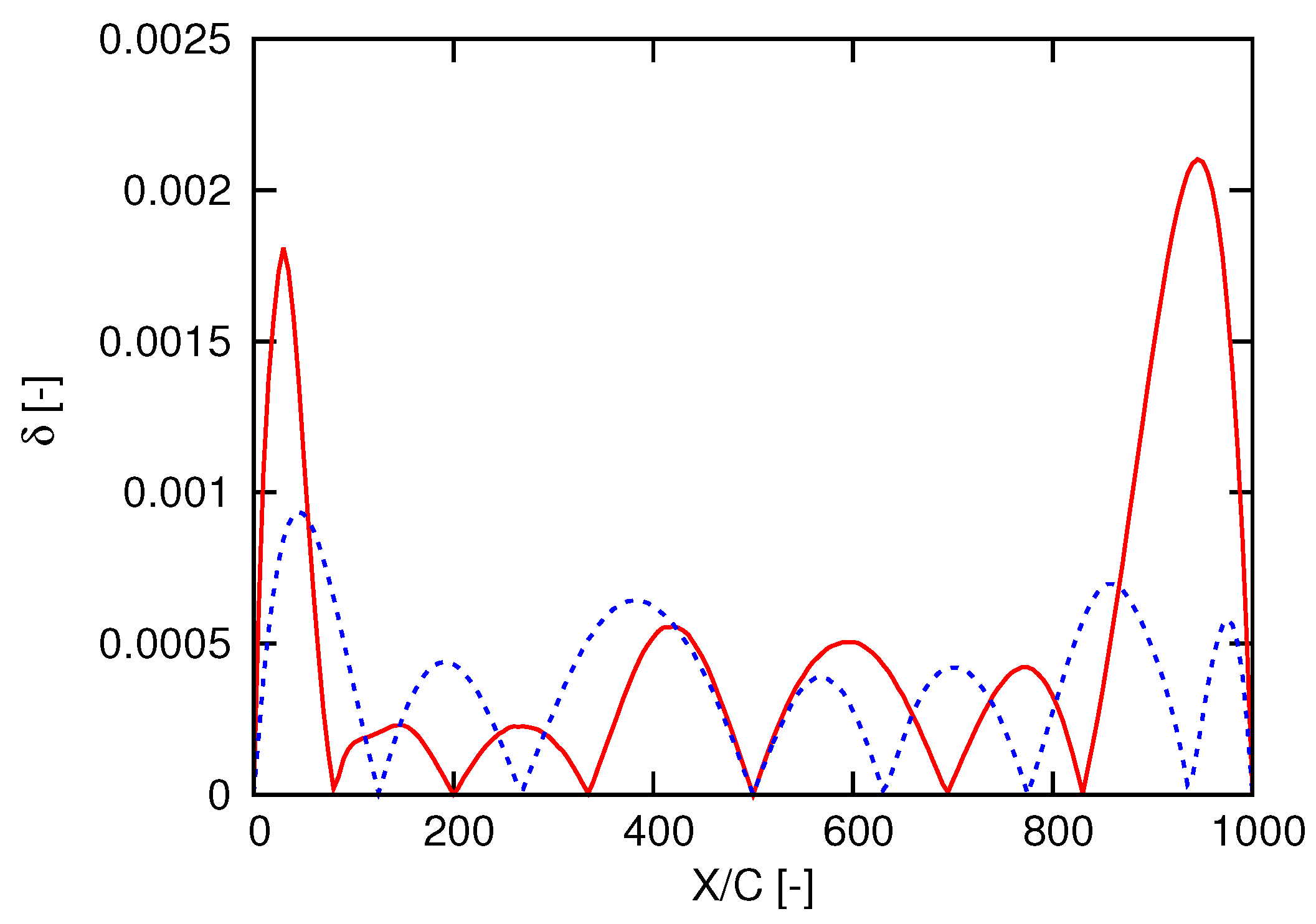
In order to determine mathematically how effectively the reference hydrofoil was parameterized, curve deviation analysis [6] was performed using the formula below:
where is the normalized deviation of the Y-coordinates of the Bezier curve from that of the reference hydrofoil at any point i, is the deviation value of the parameterized hydrofoil with respect to the reference hydrofoil at i, and l is the chord length of the original hydrofoil.
It can be seen in Figure 3 that of the upper and the lower surfaces over X/C are less than and , respectively. The deviation is negligible, and thus the parameterization technique is accurate enough to represent the reference hydrofoil and to carry out shape optimization.
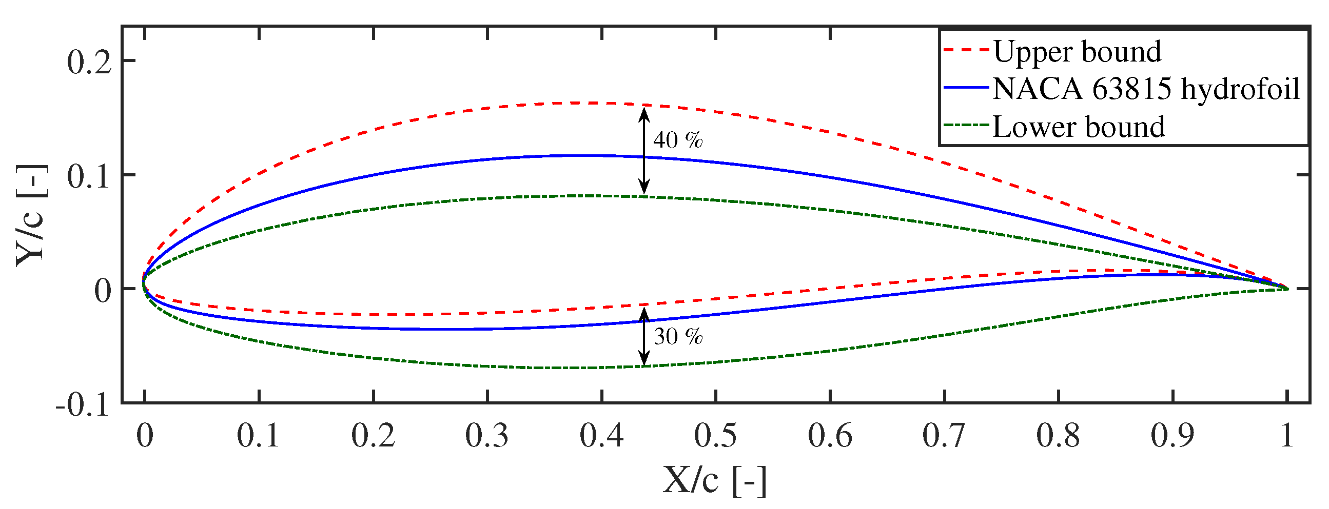
To maintain a realistic shape of the hydrofoil, constraints on its thickness are employed as shown in Figure 4. A major concern with using flow solvers is making the hydrofoil shape smooth enough, which helps to get fast converge solution. Another concern is that if the upper and the lower bounds are too wide or too narrow, the hydrofoil may not be continuous at the leading edge. Therefore, the constraints must be chosen with care. The maximum thicknesses of both the pressure and suction sides are allowed to increase and decrease by 40% and 30%, respectively, with respect to its chord. Here, the upper and lower bounds were chosen through trial and error on flow solver. The constraints have been particularly limited near the trailing edge to ensure that the curves of the pressure and suction sides do not intersect during optimization. The leading and trailing edge coordinates of the hydrofoil are fixed. Further, the x-axis coordinates of all the control points are fixed. Only the y-coordinates of the ten control points shown in Figure 2 are allowed to vary during optimization.
2.2. The Flow Solver
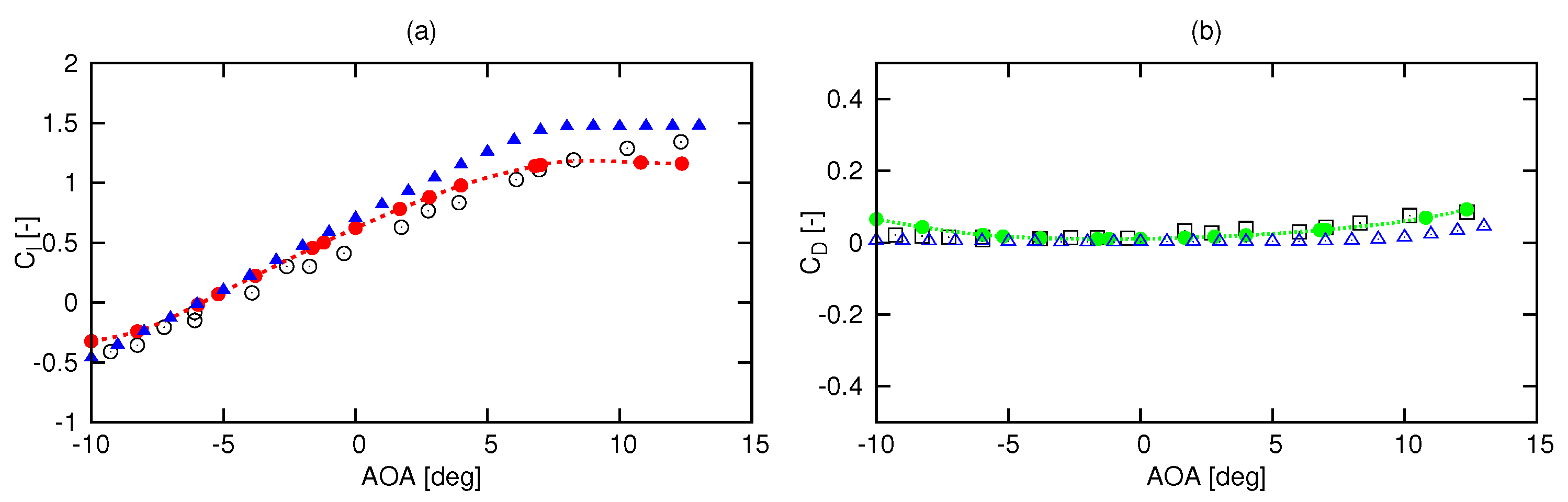
Some researchers use Computational Fluid Dynamics and many others use 2-D panel code, for instance, XFOIL [24], as the flow solver. In this study, we have compared the results of both the methods with the experimental data. The experimental results of performance characteristics of NACA 63815 were obtained from [25] for a Reynolds number of 0.8 × 10⁶ and for a flow velocity of 3.492 m/s. The computational domain for evaluating the performance characteristics of the hydrofoil using CFD simulation was set as described in [6]. The CFD simulation was performed in a 2D environment. The mesh size was set to 198,000 cells with a y+ value of 0.88. The SST turbulence model [26] was chosen to close RANS equations. The SIMPLE algorithm [27] was used for pressure–velocity coupling. Fifteen different Angles Of Attack (AOA) ranging from −10° to 12.5° were considered for the CFD simulations. The Reynolds number in XFOIL was set to 8 × 10+5 and the maximum number of iterations for the analysis of each of the hydrofoils was set to 500. The performance characteristics were evaluated in viscous mode. As shown in Figure 5, the CFD results are closer to the experimental measurements than that of XFOIL. However, the computational time using CFD was approximately 4 h, while using XFOIL it were merely 90 s. We tested almost 2480 optimized hydrofoils (30 generations and each generation has 80 hydrofoils), and to this end we needed a method that gives acceptable results within a short span of time. Furthermore, the performance predictions of XFOIL were also found to match the experimental results closely and it is also simple to use. Therefore, XFOIL was chosen as the flow solver [8,16,18,23,28].
2.3. Optimization Algorithm
In this algorithm, the solutions are sequenced based on their degree of non-domination and sent to the next generation. A simple GA consists of three genetic operators: selection, crossover, and mutation. Selection is a process in which pairs of candidate solutions are selected to reproduce. The pairs are selected based on their fitness scores. This operator is an artificial version of Darwinian’s natural selection. The tournament selection method has been used to perform the selection operation. This method was chosen as it has better convergence and computational time compared to a lot of other methods. In this method, two candidate solutions are picked randomly and their ranks are compared. The candidate solution that has better rank is selected and the other one is rejected. This process continues until all the candidate solutions are analyzed. Here, two hydrofoils are picked randomly and their lift, drag, and minimum pressure coefficients are analyzed. In GA, the next generation’s solutions are created by exchanging information among strings of the previous generation. This process is known as crossover and it is equivalent to reproduction in evolutionary biology. The crossover operation was performed by Simulated Binary Crossover (SBX). Mutation is the process in which the strings of the offspring are occasionally altered. Its main purpose is to maintain diversity in the population. Here, the polynomial mutation was performed [29].
2.4. Selection of Pareto Optimal Solutions
The optimization algorithm generated a lot of optimized hydrofoils with varied GR and cavitation characteristics. Each of the generated hydrofoils is better off with regard to one objective but is worse off with regard to another objective. Therefore, they are called Pareto-optimal solutions. The hydrofoil with the highest GR over a wide range of AOA was selected to model the optimized turbine.
2.5. The Stopping Criterion
In GAs, either of the two following approaches is employed to set the stopping criterion. First, the algorithm is set to stop if the solutions of the next generation are insignificant compared to that of its previous generation. Second, the maximum number of generations is set to a predefined value. Here, the second approach was adopted and the stopping criterion was set to 30 generations. It is a straightforward approach and was employed by taking into account the computational time. The optimized hydrofoils were generated until the stopping criterion was met. For more details, refer to the work in [30].
3. Hydrofoil Shape Optimization Strategies
The 2-D shape optimization of hydrofoil was done by considering three parameters: , , and minimum pressure coefficient (). Here, optimization was carried out to maximize and minimize in order to increase the output power of a tidal stream turbine. The optimization algorithm also sought to increase the to improve its cavitation performance [6]. Considering different AOA in the optimization algorithm generates optimized hydrofoils with different performance characteristics. Mukesh et al. [4] carried out the shape optimization for an AOA of 5°. However, the authors of [6] argued that the shape optimization done at a single AOA often results in poor performance at off-design conditions. Therefore, the authors of [6] performed the optimization for AOA of 0°, 6°, and 12°. The AOA in the optimization algorithm must therefore be chosen with care, and therefore its effect was studied in the following sections. The effect of number of objectives and its implication on the solutions was also studied.
3.1. Three Dimensional (3-D) Optimization
The main idea behind 3-D optimization was to handle each of the objectives individually, i.e., , and . Two cases were considered to study the effect of AOA. In the first case a wide range of five AOA were considered and in the second case three AOA were considered. In the first case, the objective is to maximize the average and and to minimize the average at AOA of 0°, 3°, 6°, 9°, and 12° for the objective functions shown in Equations (3)–(5). , , and were averaged to give equal weightage to all the AOA considered.
where N is the number of different AOA considered. Table 1 shows the comparison of performance characteristics of the hydrofoils that were generated in the first case.
Every generation consists of 80 hydrofoils. The mean values were taken in order to assess the efficacy of the optimization algorithm in generating hydrofoils with higher and and lower . The hydrofoils with and greater than the reference hydrofoil and lesser than the reference hydrofoil were designated as optimized hydrofoils in each generation. The mean and of the hydrofoils in the last generation is higher than that of the first generation and the mean is lower, which indicates that the optimization algorithm could generate better hydrofoils as the execution of the optimization code progresses.
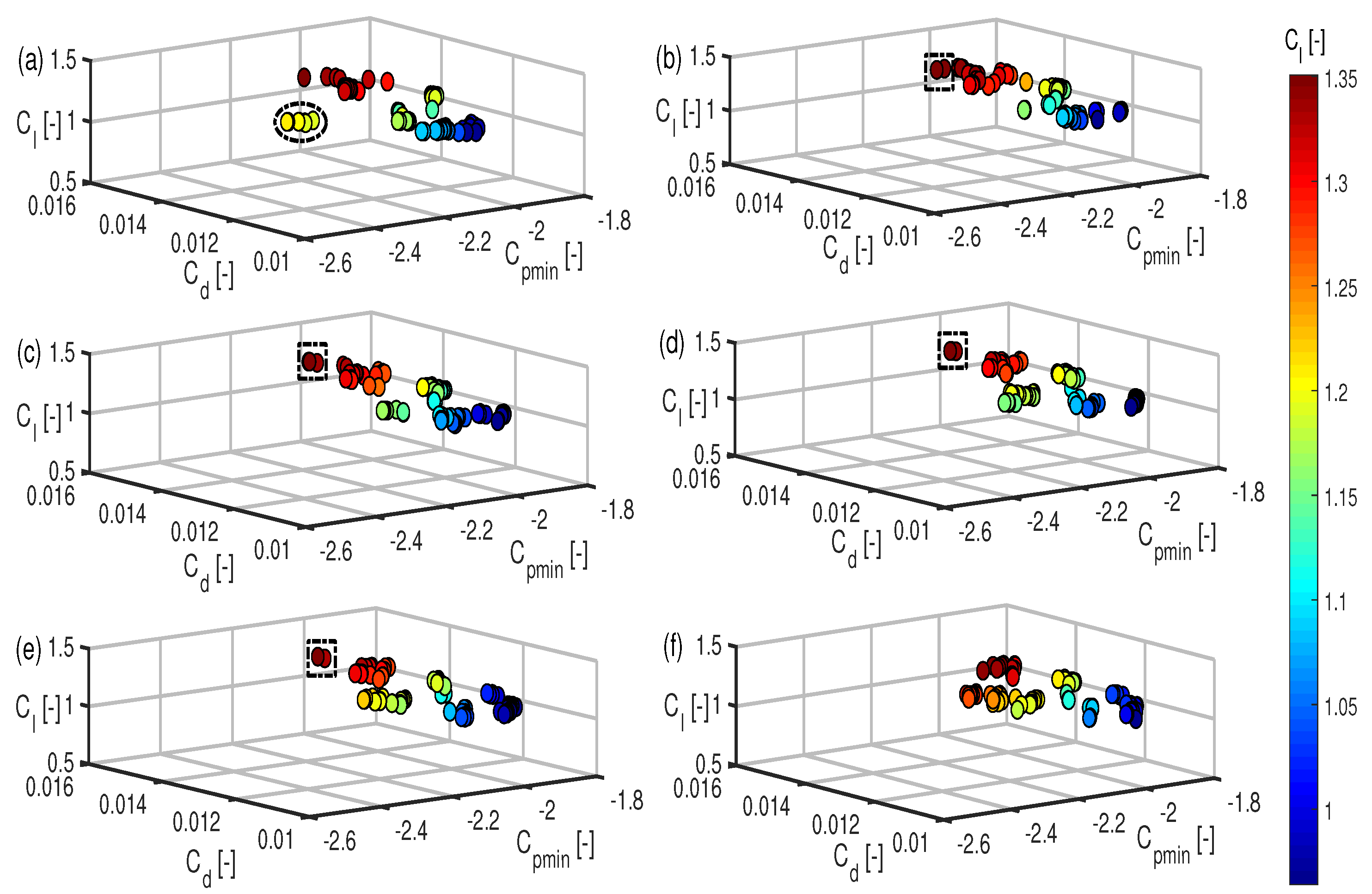
The 3D Pareto-optimal graphs of the first case for different generations are shown in Figure 6. The hydrofoil characteristics are color-coded according to their values. Figure 6a shows performance characteristics of optimized hydrofoils obtained in the 5th generation. Seven hydrofoils are shown within a dotted black ellipse, which have poor cavitation characteristics relative to the others in the same generation. Their ranges from −2.438 to −2.359, ranges from 0.117 to 0.012, and ranges from 1.19 to 1.22. However, as some hydrofoils overlap another, only four of them are visible. In the 10th generation, as shown in Figure 6b, the seven hydrofoils were excluded and were replaced with hydrofoils having better cavitation characteristics. Three hydrofoils that are shown within dotted black rectangles in Figure 6b–e having ranging from 1.35 to 1.4 and ranging from 0.014 to 0.0142 were retained until the 25th generation. Although they have the worst values, they were retained until the 25th generation owing to their high values. They were eventually replaced with hydrofoils having lower and higher in the 30th generation as shown in Figure 6f. In course of the execution of the optimization code, the of the generated hydrofoils gradually became lesser compared to its preceding generations.
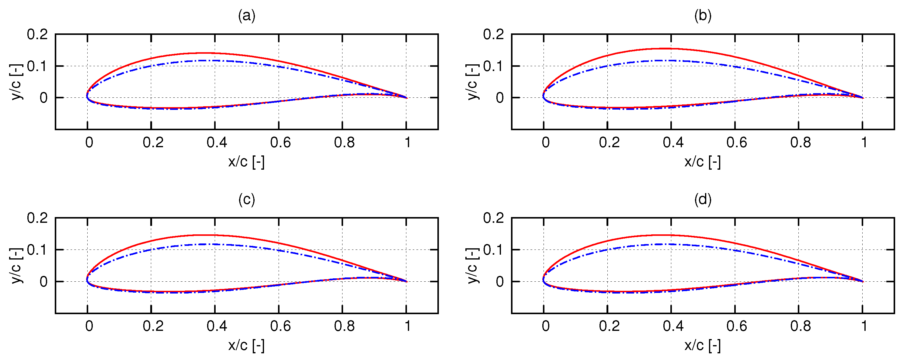
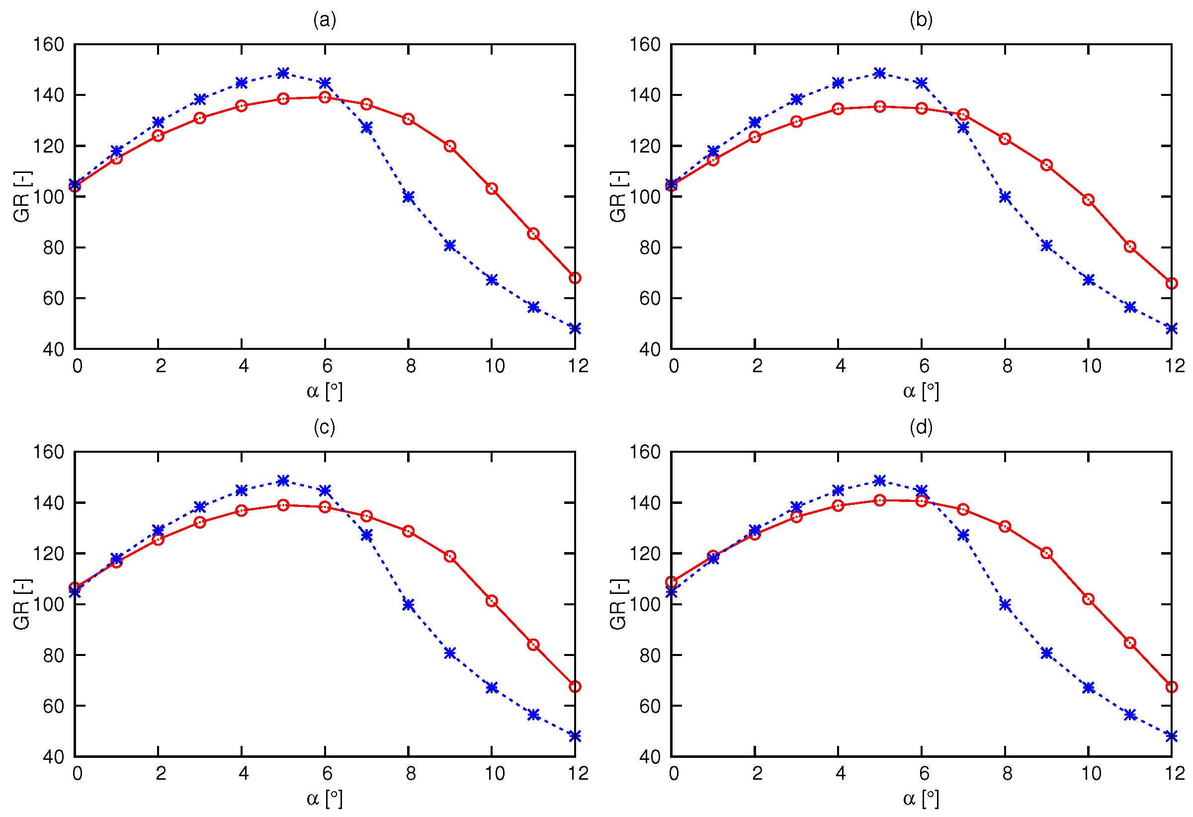
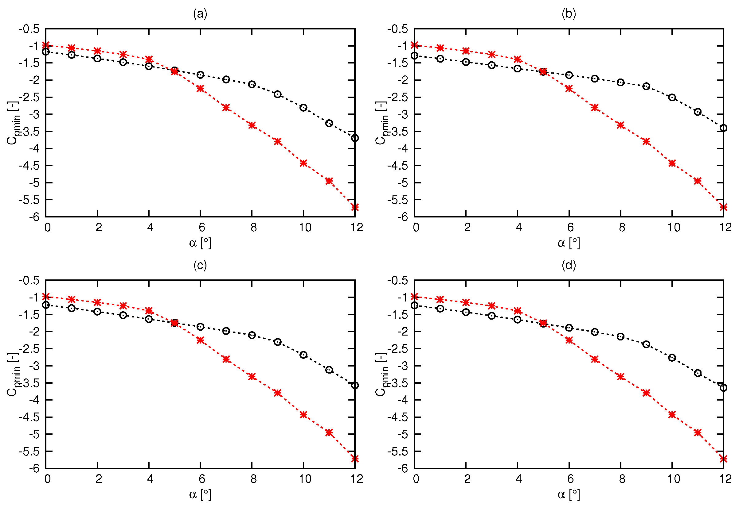
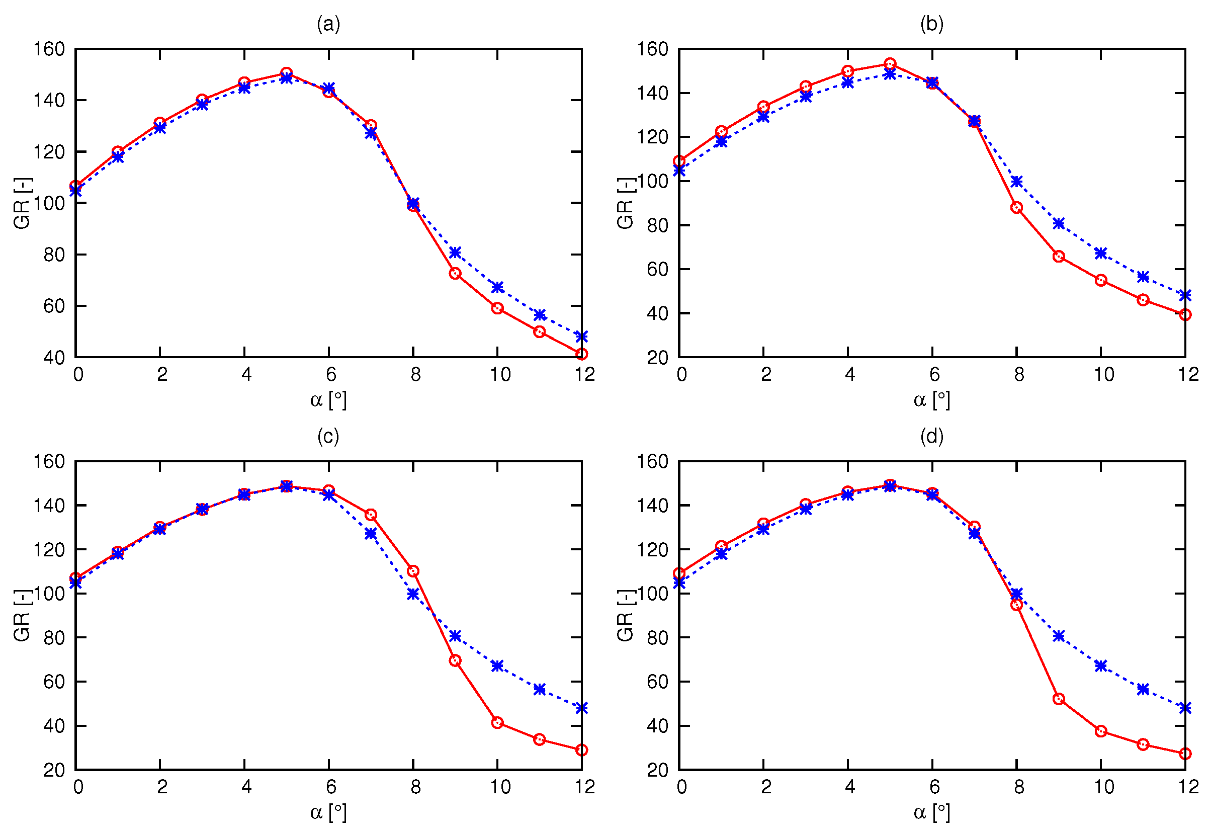
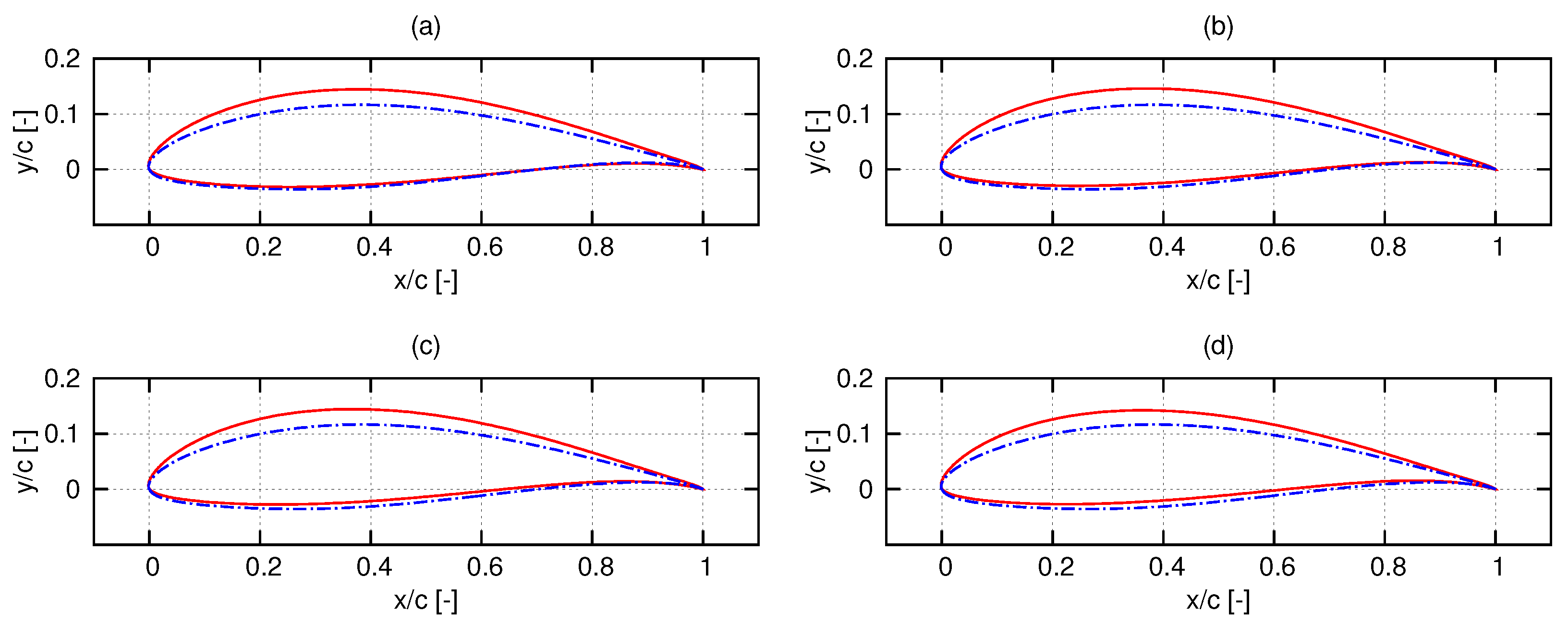
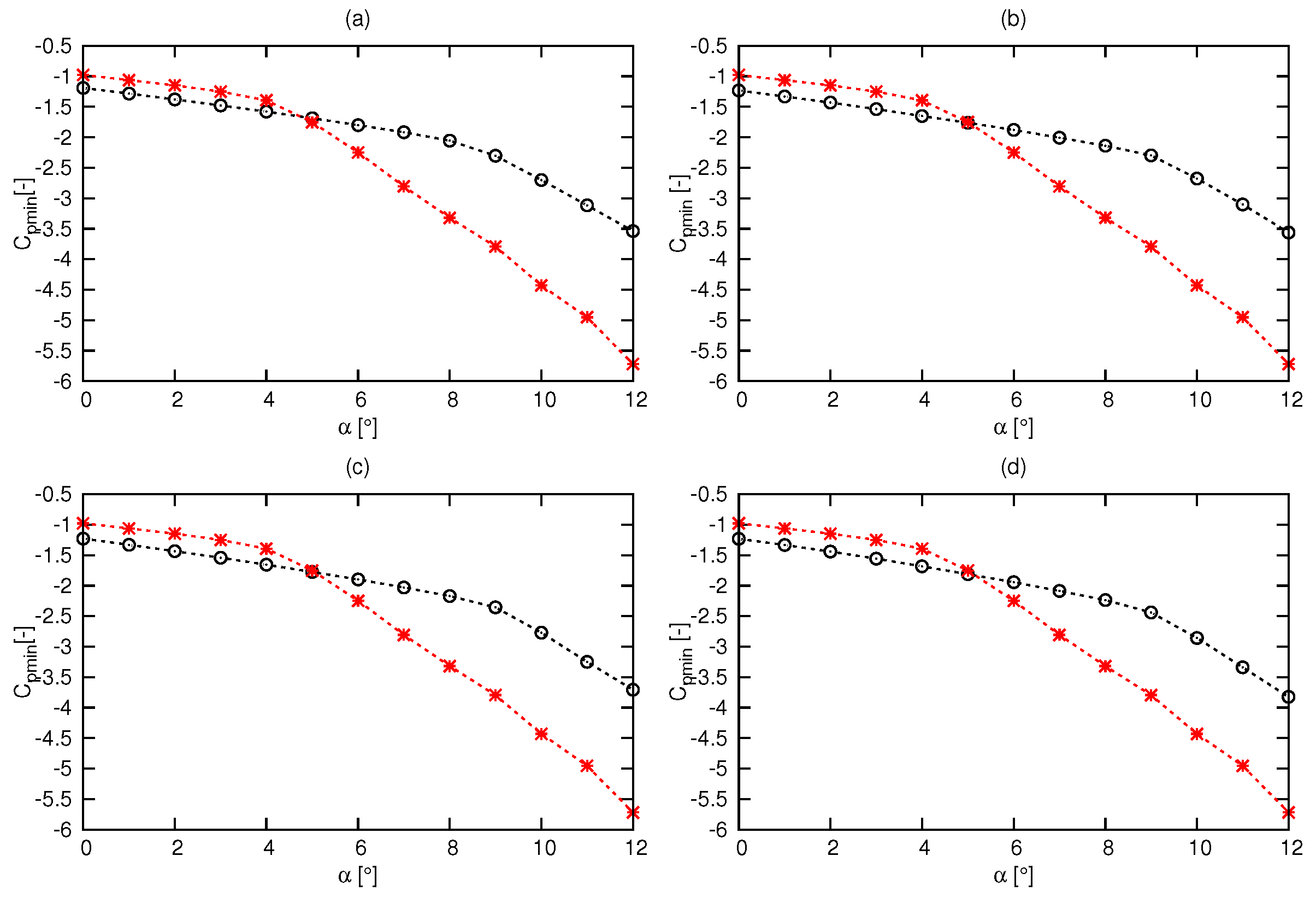
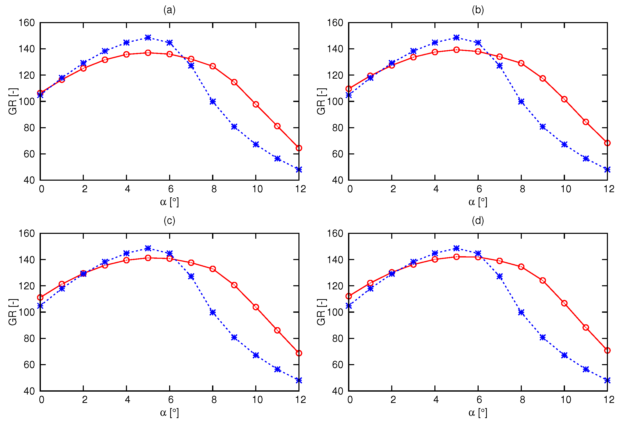
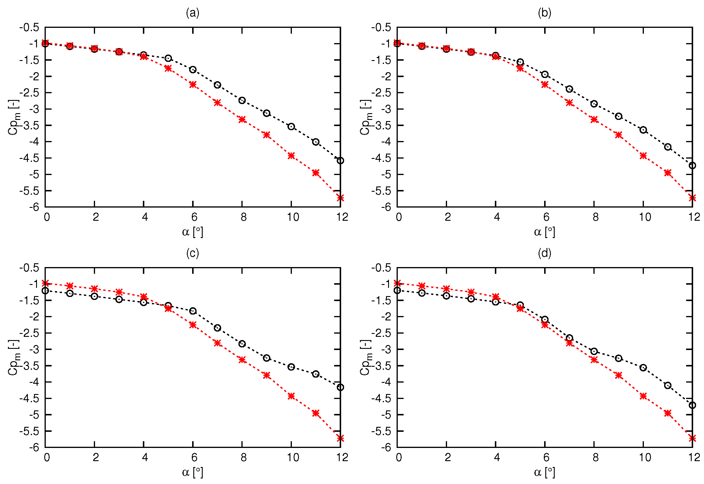
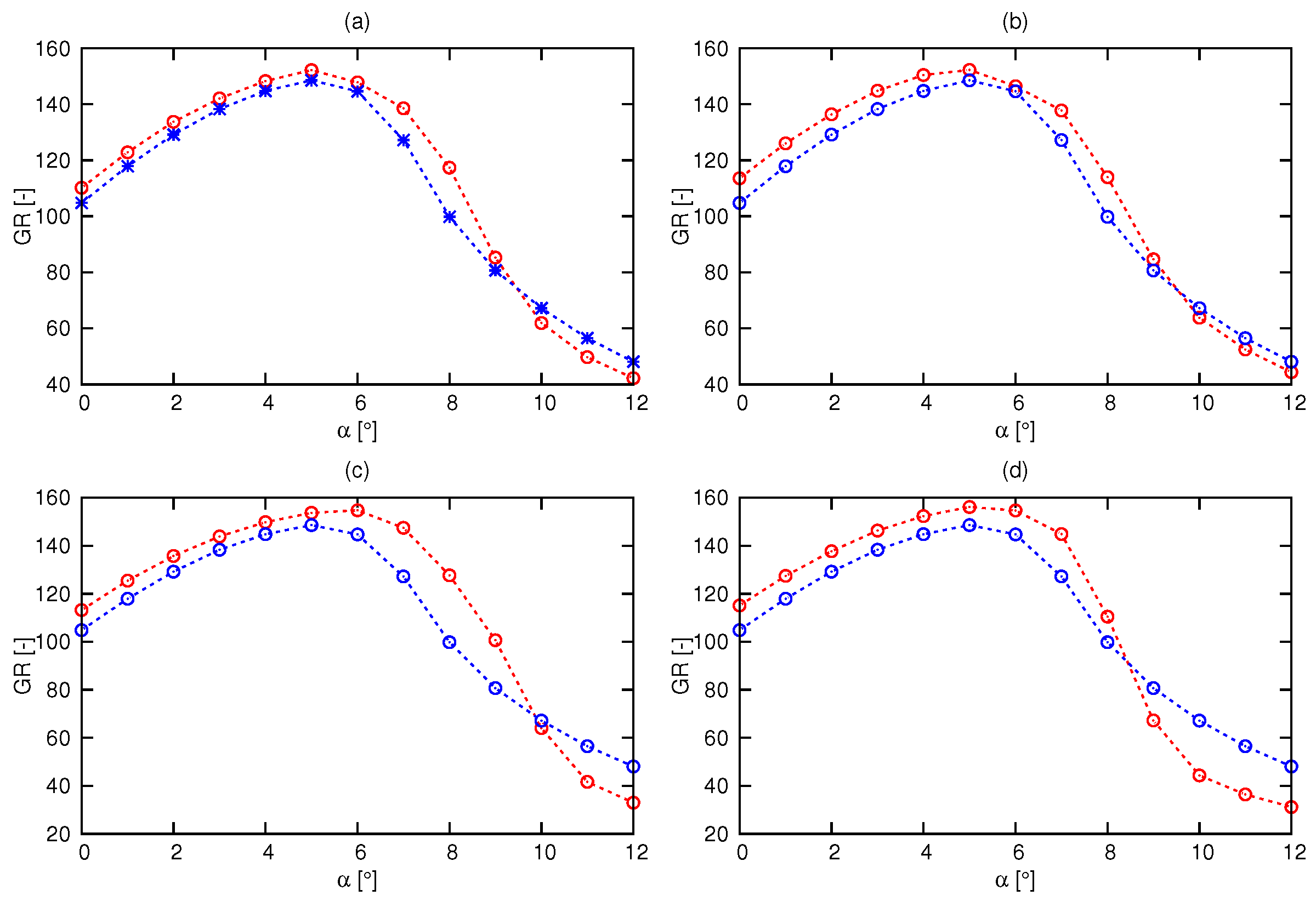
Four hydrofoils with the highest GR are shown in Figure 7. Figure 7a shows an optimized hydrofoil ( HF-3D-1-1), which has maximum thickness () of 17.09% at 33.7% of the chord length from the leading edge (). Here, HF refers to hydrofoil, 3D refers to three-dimensional optimization, the first 1 refers to the first case, and the second 1 refers to the first optimized hydrofoil. It can be seen in Figure 8a that the HF-3D-1-1 has a higher GR from AOA = 0° to almost 2° and from AOA = 6.1° to 12°. Figure 9a shows that of the optimized hydrofoil has been improved at higher AOA ranging from 5° to 12°. Figure 7b shows the second optimized hydrofoil (HF-3D-1-2), which has of 18.26% at 0.347 c. It can be seen from Figure 8b that the optimized hydrofoil has a higher GR from AOA = 0° to 1° and from AOA = 6.2° to 12°. Figure 9c shows that the cavitation performance of the optimized hydrofoil is closer to that of the reference hydrofoil at lower AOA and from AOA of 5° the cavitation performance has been greatly improved. Figure 7c shows the third optimized hydrofoil (HF-3D-1-3), which has of 17.58% at 0.339 c. It can be seen from Figure 8c that the optimized hydrofoil has a higher GR from AOA = 0° to 1° and from AOA = 6.2° to 12°. Figure 9b shows that the cavitation performance of the optimized hydrofoil is closer to the reference hydrofoil at lower AOA and from AOA = 5° the cavitation performance has been greatly improved. Figure 7d shows the fourth optimized hydrofoil (HF-3D-1-4) has of % at 0.337 c. Although Figure 8d and Figure 9d show that the GR and were not improved at lower AOA, it performs well at higher AOA.
In the first case, hydrofoils were produced that performed consistently well at wide range of AOA. The GR and the cavitation performance were improved at higher AOA. However, the maximum GR of the optimized hydrofoils were lower than the reference hydrofoil, which is undesirable.
As the maximum GR of the reference and the optimized hydrofoils in the previous case lie between AOA of 4° and 6°, the optimization was done at these AOA with a focus on increasing the maximum GR. Equations (3), (4), and (6) are calculated for AOA of 4°, 5°, and 6°.
It can be seen in Figure 10 that the optimized hydrofoils of this case have higher GR at smaller AOA than the hydrofoils obtained in the first case (Figure 8), wherein the optimized hydrofoils had better performance characteristics only at higher AOA. As shown in Figure 11, the cavitation performance is better than in the first case (Figure 9). It, however, turned out that the Pareto optimal solutions are not as diverse as the first case.
3.2. Two-Dimensional (2-D) Optimization
It is possible that the process of evolution of the optimized hydrofoils was slowed down on account of it being a high-dimensional multi-objective optimization problem. The number of objectives was, therefore, reduced to two by considering and GR as the optimization objectives as shown Equations (5) and (6) respectively.
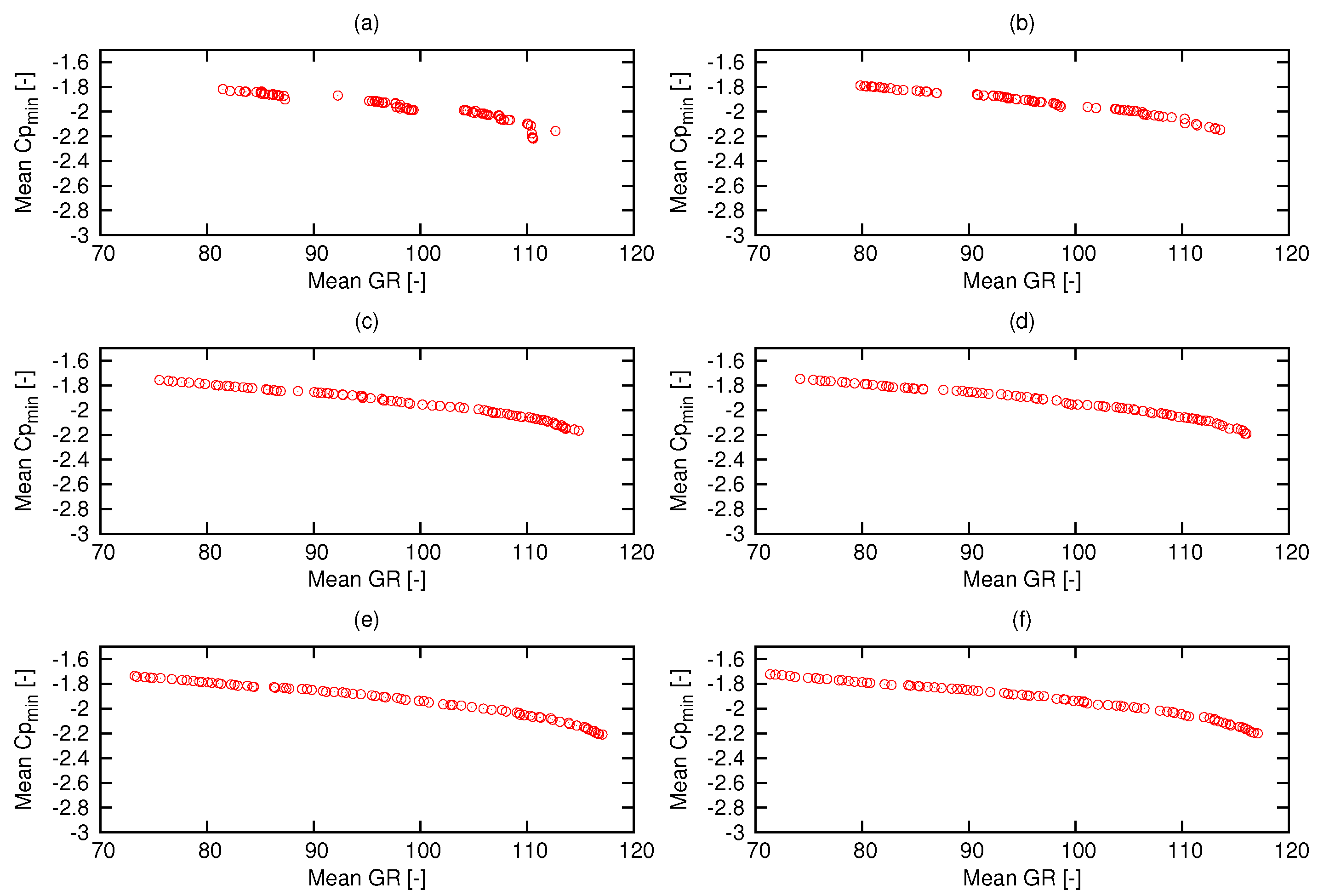
where is the summation of GR at different AOA. In this case, the summation of GR and are calculated at AOA of 0°, 3°, 6°, 9°, and 12°. Table 2 shows the comparison of the performance characteristics of the hydrofoils in different generations. The mean GR and values show only the general behaviour of the optimization algorithm, which sporadically increase and decrease for two reasons. First, optimization was done by considering two conflicting objectives, i.e., improvement in one objective is achieved at the expense of the other objective. Second, the crowding distance operator was used to diversify the solutions at the end of each generation. In Table 2, it can be seen that in the 5th generation the number of optimized hydrofoils is higher than all the other generations. For better clarity refer to Figure 12a, which shows that the hydrofoil characteristics of this generation are bunched together meaning that some of the optimized hydrofoils are almost similar. The duplication of hydrofoils is avoided by using the crowding distance operator whose primary task is to diversify the Pareto optimal solutions as shown in Figure 12. The distribution of the performance characteristics of hydrofoils in the 30th generation (Figure 12f) is the most diverse compared to the other generations (Figure 12a–e). With diverse solutions, the designer will have a lot of hydrofoils to choose from based on their specific requirements.
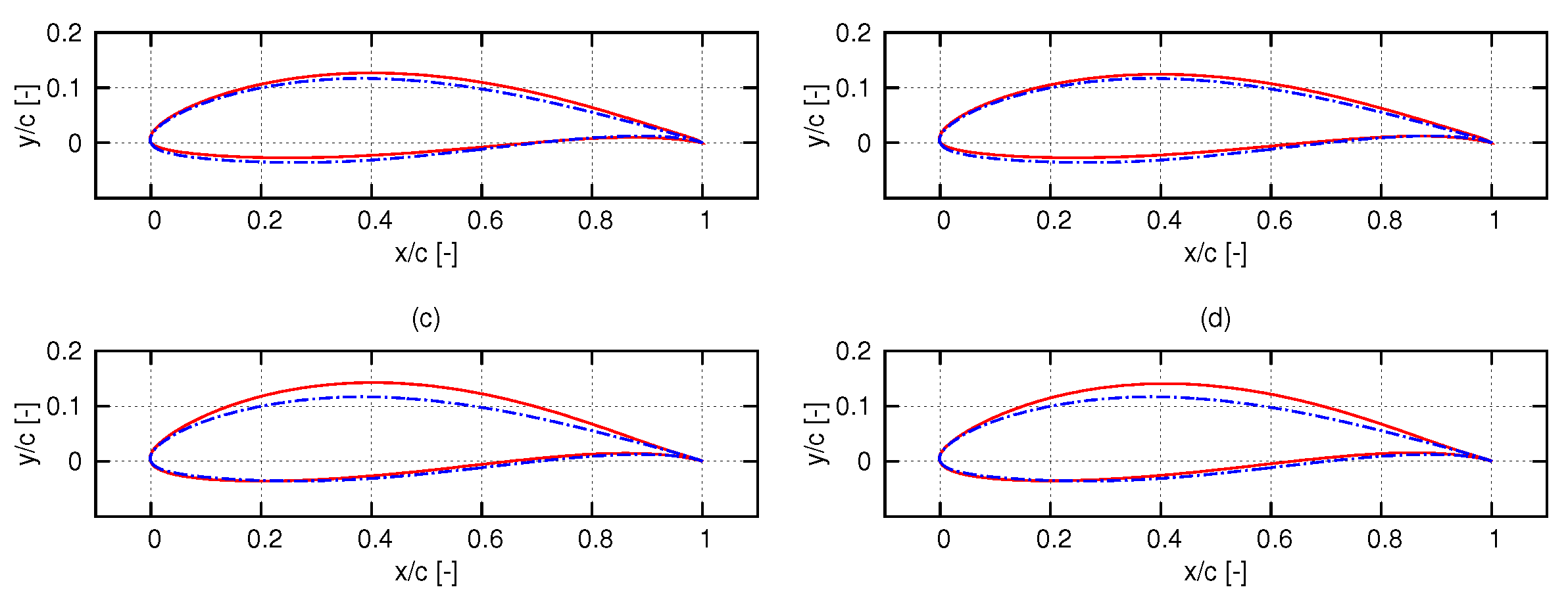
Four hydrofoils with the highest GR in the 30th generation are shown in Figure 13. The GR of hydrofoil (HF-2D-1-1) whose is % at 0.303 c is shown Figure 13a. The GR of this hydrofoil is higher than that of the reference hydrofoil from AOA = 0° to 2° and from AOA = 6.2° to 12° as shown in Figure 14a. The cavitation performance is better from AOA greater than 5° as shown in Figure 15a. The second optimized hydrofoil (HF-2D-1-2) in Figure 13b has of % at . The GR of this hydrofoil is higher than the reference hydrofoil from AOA = 0° to 2° and from AOA = 6.2° to 12° as shown in Figure 15b. The cavitation performance is better from AOA greater than 5° as shown in Figure 14b. The third optimized hydrofoil (HF-2D-1-3) shown in Figure 13c has of % at as shown in Figure 15c. The GR of the hydrofoil is higher than the reference hydrofoil from AOA = 0° to 2° and from AOA = 6.2° to 12°, and the cavitation performance is better from AOA greater than 5° as shown in Figure 15c. The fourth optimized hydrofoil (HF-2D-1-4) shown in Figure 13d has of % at as shown in Figure 15d. The maximum GRs of the hydrofoils obtained in this case are lower than the reference hydrofoil, but they have better cavitation characteristics at higher AOA as shown in Figure 14d. By reducing the number of objectives to two, a marked improvement in the performances of the hydrofoils could be noticed.
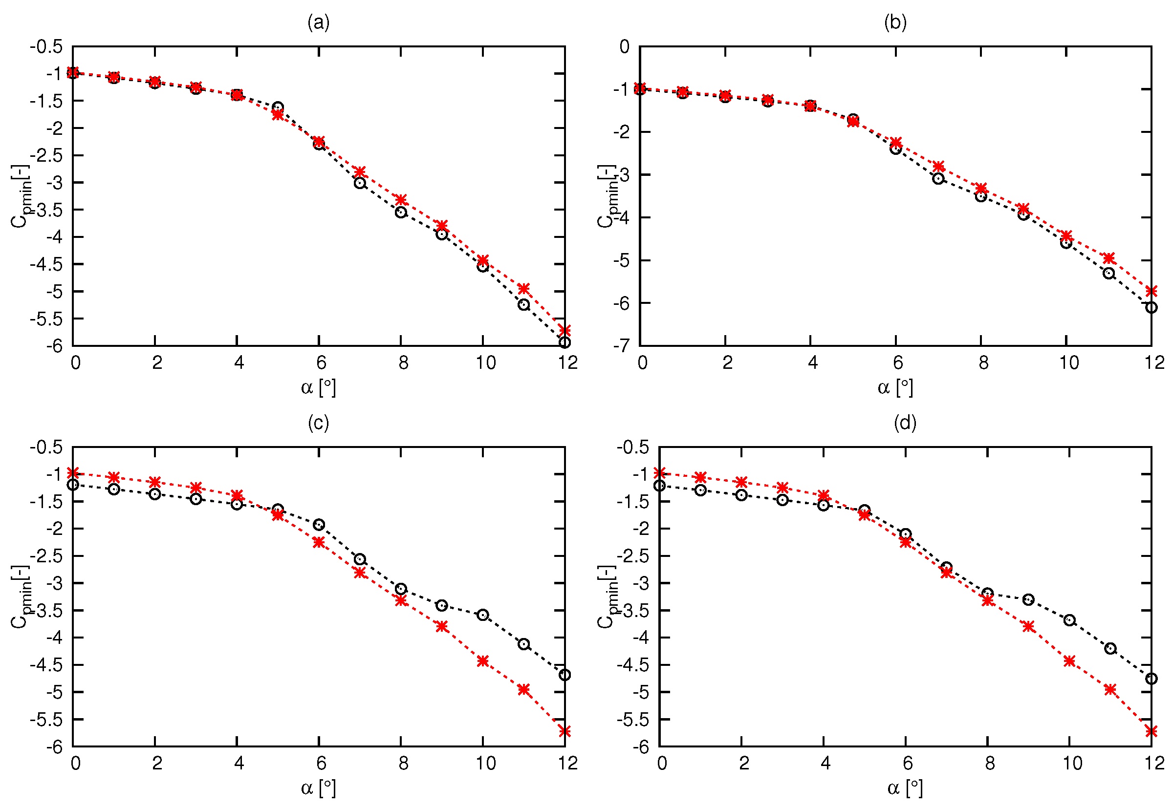
Further, the maximum GRs lie between AOA 4 and 6. Therefore, 2D optimization was done for these AOA. Equations (5) and (6) are calculated for AOA of 4°, 5°, and 6°. Four hydrofoils with the highest GR are shown in Figure 16. The GR of HF-2D-2-1 that is shown in Figure 16a is higher than that of the reference hydrofoil from AOA 0° to 8° and the is greater from AOA greater than 5° as shown in Figure 17a and Figure 18a, respectively. The GR of the second hydrofoil (HF-2D-2-2) is higher than that of the reference hydrofoil from AOA 0° to 9.8° and the cavitation performance is better from AOA greater than 5° as shown in Figure 17b and Figure 18b, respectively. The third optimized hydrofoil (HF-2D-2-3) whose is % at is shown in Figure 13c. The GR of this hydrofoil is significantly higher than the reference hydrofoil from AOA 0° to almost 10° and the cavitation performance was better than the reference hydrofoil from AOA greater than 5°. The performance characteristics of the fourth hydrofoil (HF-2D-2-4) are not as good as the previous two hydrofoils but still are better than the reference hydrofoil, especially with regard to the GR from AOA 0° to 8°. The GRs of the hydrofoils obtained in this case are also higher than that of all the optimized hydrofoils in the previous three cases. On the other hand, the cavitation performances are not as good as that of the optimized hydrofoils obtained in the first cases of 2D and 3D optimization.
Some of the optimized hydrofoils obtained in this case have GRs greater than the reference hydrofoil from AOA ranging from 0° to 10°. Further, the GRs of the hydrofoils are higher than those obtained in the other optimization cases. On the other hand, the cavitation characteristics were almost the same from 0° to 5° and after that they were improved until AOA of 12°. Although hydrofoils were generated with higher , lower , and higher , the evolution of optimized hydrofoils was slow. Further, the influence of the crowding distance operator was apparently insignificant in the 3D optimization.
4. Conclusions
The onus is on the designer of the tidal stream turbines to select hydrofoils based on their specific requirements.
An in-house MATLAB code was developed based on [11] to perform shape optimization of hydrofoils by employing NSGA-2 algorithm and coupled with a flow solver. The hydrofoil was parameterized using 6th order Bezier curves. In that case, NACA 63815 was taken as a reference hydrofoil. The maximum normalized deviation of the Bezier parameterized reference hydrofoil from the original hydrofoil was accurate enough to carry out shape optimization.
For the chosen solver, the 2D panel method XFOIL solver and CFD results of Lift and drag coefficients of the reference hydrofoil were compared with the experimental measurements. The results for CFD is more accurate but also more time consuming, thus the XFOIL solver was chosen on account of its simplicity and its ability to give acceptable results within a short span of time compare to CFD.
A comparative study on the optimization was done by considering two methods. For 3D optimization, three objective, i.e., , and , were the optimization objectives, and for 2D optimization, the number of objectives was reduced to two by unifying and as GR. The GR of the hydrofoils was further improved by performing optimization at AOA of 4°, 5° and 6° than on performing at AOA of 0°, 3°, 6°, 9°, and 12°.
This was because the maximum glide ratio of reference hydrofoil fell within the range of 4° and 6°. However, the cavitation characteristics were better at higher AOA in the first case.
The multi-objective optimization performed in the present work effectively improved the GR of the hydrofoils from AOA of 0° to almost 10°. The cavitation performance was mainly improved from AOA 5° to 12°. The solutions of optimization are not unique. Different hydrofoils with different performance characteristics were obtained, but a lot of them performed better than NACA 63815.
Author Contributions
H.e.S.: Conceptualization, methodology, visualization, writing and review, editing; S.N.: Conceptualization, methodology, software, formal analysis, visualization, original draft preparation, editing; O.e.M.: supervision and writing and review. All authors have read and agreed to the published version of the manuscript.
Funding
This research received no external funding.
Conflicts of Interest
The authors declare no conflict of interest.
References
- Nemec, M.; Zingg, D.W.; Pulliam, T.H. Multipoint and multi-objective aerodynamic shape optimization. AIAA J. 2004, 6, 1057–1065. [Google Scholar] [CrossRef]
- Peigin, S.; Epstein, B. Robust optimization of 2d airfoils driven by full Navier–Stokes computations. Comput. Fluids 2004, 9, 1175–1200. [Google Scholar] [CrossRef]
- Shahrokhi, A.; Jahangirian, A. Airfoil shape parameterization for optimum Navier–Stokes design with genetic algorithm. Aerosp. Sci. Technol. 2007, 6, 443–450. [Google Scholar] [CrossRef]
- Mukesh, R.; Lingadurai, K.; Selvakumar, U. Airfoil shape optimization using non-traditional optimization technique and its validation. J. King Saud Univ.-Eng. Sci. 2014, 2, 191–197. [Google Scholar] [CrossRef] [Green Version]
- Ribeiro, A.; Awruch, A.M.; Gomes, H.M. An airfoil optimization technique for wind turbines. Appl. Math. Model. 2012, 10, 4898–4907. [Google Scholar] [CrossRef]
- Luo, X.-Q.; Zhu, G.-J.; Feng, J.-J. Multi-point design optimization of hydrofoil for marine current turbine. J. Hydrodyn. Ser. B 2014, 5, 807–817. [Google Scholar] [CrossRef]
- Liu, P.; Veitch, B. Design and optimization for strength and integrity of tidal turbine rotor blades. Energy 2012, 1, 393–404. [Google Scholar] [CrossRef]
- Goundar, J.N.; Ahmed, M.R. Design of a horizontal axis tidal current turbine. Appl. Energy 2013, 111, 161–174. [Google Scholar] [CrossRef]
- Papadrakakis, M.; Papadopoulos, V.; Stefanou, G.; Plevris, V.A. Framework for the design by optimization of hydrofoils under cavitating conditions. In Proceedings of the 7th European Congress on Computational Methods in Applied Sciences and Engineering, ECCOMAS 2016, Crete, Greece, 5–10 June 2016. [Google Scholar]
- De Boor, C.; Mathematicien, E.-U.; De Boor, C. A Practical Guide to Splines; Springer: New York, NY, USA, 1978; Volume 27. [Google Scholar]
- Deb, K.; Pratap, A.; Agarwal, S.; Meyarivan, T.A.M.T. A fast and elitist multiobjective genetic algorithm: NSGA-II. IEEE Trans. Evol. Comput. 2002, 2, 182–197. [Google Scholar] [CrossRef] [Green Version]
- Clerc, M. Particle Swarm Optimization; John Wiley & Sons: Hoboken, NJ, USA, 2010. [Google Scholar]
- Kennedy, J.; Eberhart, R. Particle swarm optimization. Int. Conf. Neural Netw. 1995, 5, 1942–1948. [Google Scholar]
- Hsin, C.-Y.; Wu, J.-L.; Chang, S.-F. Design and optimization method for a two-dimensional hydrofoil. J. Hydrodyn. 2006, 5, 323–329. [Google Scholar] [CrossRef]
- Ouyang, H.; Weber, L.J.; Odgaard, A.J. Design optimization of a two-dimensional hydrofoil by applying a genetic algorithm. Eng. Optim. 2014, 5, 529–540. [Google Scholar] [CrossRef]
- Zhang, D.-S.; Chen, J.; Shi, W.-D.; Shi, L.; Geng, L.-L. Optimization of hydrofoil for tidal current turbine based on particle swarm optimization and computational fluid dynamic method. Therm. Sci. 2016, 3, 907–912. [Google Scholar] [CrossRef]
- Litvinov, W. On the optimal shape of a hydrofoil. J. Optim. Theory Appl. 1995, 2, 325–345. [Google Scholar] [CrossRef]
- Goundar, J.N.; Ahmed, M.R.; Lee, Y.-H. Numerical and experimental studies on hydrofoils for marine current turbines. Renew. Energy 2012, 42, 173–179. [Google Scholar] [CrossRef]
- Tahani, M.; Babayan, N. Optimum section selection procedure for horizontal axis tidal stream turbines. Neural Comput. Appl. 2017, 31, 1211–1223. [Google Scholar] [CrossRef]
- Konak, A.; Coit, D.W.; Smith, A.E. Multi-objective optimization using genetic algorithms: A tutorial. Reliab. Eng. Syst. Saf. 2006, 91, 992–1007. [Google Scholar] [CrossRef]
- Baskar, S.; Tamilselvi, S.; Varshini, P. MATLAB Code for Constrained NSGA II. Available online: https://de.mathworks.com/matlabcentral/fileexchange/49806-matlab-code-for-constrained-nsga-ii-dr-s-baskar–s-tamilselvi-and-//mdx.plm.automation.siemens.com/star-ccm-plus/ (accessed on 12 October 2017).
- Abbott, I.H.; von Doenhoff, A.E. Theory of Wing Sections, Including a Summary of Airfoil Data; Courier Corporation: Mineola, NY, USA, 1959. [Google Scholar]
- Batten, W.; Bahaj, A.; Moll, A.; Chaplin, J. Hydrodynamics of marine current turbines. Renew. Energy 2006, 31, 249–256. [Google Scholar] [CrossRef] [Green Version]
- Drela, M. Xfoil: An Analysis and Design System for Low Reynolds Number Airfoils; Springer: Berlin/Heidelberg, Germany, 1989; Volume 111, pp. 1–12. [Google Scholar]
- Moll, A.F.; Bahaj, A.S.; Chaplin, J.R.; Batten, W.M.J. Measurements and predictions of forces, pressures and cavitation on 2-D sections suitable for marine current turbines. Proc. Inst. Mech. Eng. Part M 2004, 2, 127–138. [Google Scholar]
- Menter, F. Zonal two equation kw turbulence models for aerodynamic flows. In Proceedings of the 23rd Fluid Dynamics, Plasma Dynamics, and Lasers Conference, Orlando, FL, USA, 6–9 July 1993. [Google Scholar]
- Patankar, S.V. Computational Methods for Fluid Dynamics; Taylor& Francis: Germantown, NY, USA, 2016. [Google Scholar]
- Batten, W.M.J.; Bahaj, A.S.; Moll, A.F.; Chaplin, J.R. Experimentally validated numerical method for the hydrodynamic design of horizontal axis tidal turbines. Ocean. Eng. 2007, 7, 1013–1020. [Google Scholar] [CrossRef]
- Goldberg, D. Genetic Algorithms in Search, Optimization, and Machine Learning; Addison-Wesley Publishing Company: Boston, MA, USA, 1989. [Google Scholar]
- Deb, K. Multi-Objective Optimization Using Evolutionary Algorithms; Wiley: Hoboken, NJ, USA, 2009. [Google Scholar]
Figure 1.
Flowchart of optimization methodology.

Figure 2.
Original and Bezier curve parameterized NACA 63815 hydrofoil, where X/C and Y/C are the normalized distance in x and y directions to the hydrofoil chord length ratio.
Figure 2.
Original and Bezier curve parameterized NACA 63815 hydrofoil, where X/C and Y/C are the normalized distance in x and y directions to the hydrofoil chord length ratio.

Figure 3.
Curve deviation analysis of the parameterized hydrofoil, where denotes the normalized deviation of the Y-coordinates of the parameterized hydrofoil from that of the reference hydrofoil and X/C denotes the distance in x-direction normalized to the hydrofoil chord length. The dotted blue line represents the deviation in the suction side and the solid red line represents the deviation in the pressure side.

Figure 4.
Optimized hydrofoil with upper and lower bounds for the optimization.

Figure 5.
Comparison of RANS (red and green dots) and XFOIL (blue and green triangles) results with the experimental values, where (a) represents lift coefficients (Cl) vs. angles of attack (AOA) and (b) represents drag coefficients (Cd) vs. AOA.
Figure 5.
Comparison of RANS (red and green dots) and XFOIL (blue and green triangles) results with the experimental values, where (a) represents lift coefficients (Cl) vs. angles of attack (AOA) and (b) represents drag coefficients (Cd) vs. AOA.

Figure 6.
3-D Pareto optimal graph of the different generations, where (a) represents the 5th, (b) represents the 10th, (c) represents the 15th, (d) represents the 20th, (e) represents the 25th, and (f) represents the 30th generations.
Figure 6.
3-D Pareto optimal graph of the different generations, where (a) represents the 5th, (b) represents the 10th, (c) represents the 15th, (d) represents the 20th, (e) represents the 25th, and (f) represents the 30th generations.

Figure 7.
Reference and optimized hydrofoils of the first case of 3D optimization, where (a) is optimized hydrofoil HF-3D-1-1, (b) is optimized hydrofoil HF-3D-1-2, (c) is optimized hydrofoil HF-3D-1-3 and (d) is optimized hydrofoil HF-3D-1-4. The red solid lines denote the optimized hydrofoil and the blue dash-dot lines denote the original hydrofoil.

Figure 8.
GR of the reference and optimized hydrofoils of the first case of 3D optimization, where (a) is GR of HF-3D-1-1, (b) is GR of HF-3D-1-2, (c) is GR of HF-3D-1-3 and (d) is GR of HF-3D-1-4. The red and blue lines denote optimized and reference hydrofoils, respectively.
Figure 8.
GR of the reference and optimized hydrofoils of the first case of 3D optimization, where (a) is GR of HF-3D-1-1, (b) is GR of HF-3D-1-2, (c) is GR of HF-3D-1-3 and (d) is GR of HF-3D-1-4. The red and blue lines denote optimized and reference hydrofoils, respectively.

Figure 9.
of the reference and optimized hydrofoils of the first case of 3-D optimization, where (a) is of HF-3D-1-1, (b) is of HF-3D-1-2, (c) is of HF-3D-1-3, (d) is of HF-3D-1-4. The red and black lines denote optimized and reference hydrofoil, respectively.
Figure 9.
of the reference and optimized hydrofoils of the first case of 3-D optimization, where (a) is of HF-3D-1-1, (b) is of HF-3D-1-2, (c) is of HF-3D-1-3, (d) is of HF-3D-1-4. The red and black lines denote optimized and reference hydrofoil, respectively.

Figure 10.
GR of the reference and optimized hydrofoils of the second case of 3-D optimization, where (a) is GR of HF-3D-2-1, (b) is GR of HF-3D-2-2, (c) is GR of HF-3D-2-3 and (d) is GR of HF-3D-2-4. The red and blue lines denote optimized and reference, respectively.
Figure 10.
GR of the reference and optimized hydrofoils of the second case of 3-D optimization, where (a) is GR of HF-3D-2-1, (b) is GR of HF-3D-2-2, (c) is GR of HF-3D-2-3 and (d) is GR of HF-3D-2-4. The red and blue lines denote optimized and reference, respectively.

Figure 11.
of the reference and optimized hydrofoils of the second case of 3-D optimization, where (a) is of HF-3D-2-1, (b) is of HF-3D-2-2; (c) is of HF-3D-2-3, (d) is of HF-3D-2-4. The red and black lines denote optimized and reference hydrofoil, respectively.
Figure 11.
of the reference and optimized hydrofoils of the second case of 3-D optimization, where (a) is of HF-3D-2-1, (b) is of HF-3D-2-2; (c) is of HF-3D-2-3, (d) is of HF-3D-2-4. The red and black lines denote optimized and reference hydrofoil, respectively.

Figure 12.
Graphs for the different generations in the first case of 2D optimization, where (a) represents the 5th, (b) represents the 10th, (c) represents the 15th, (d) represents the 20th, (e) represents the 25th, and (f) represents the 30th generations.
Figure 12.
Graphs for the different generations in the first case of 2D optimization, where (a) represents the 5th, (b) represents the 10th, (c) represents the 15th, (d) represents the 20th, (e) represents the 25th, and (f) represents the 30th generations.

Figure 13.
Reference and optimized hydrofoils of the first case of 2-D optimization, where (a) is optimized hydrofoil HF-2D-1-1, (b) is optimized hydrofoil HF-2D-1-2, (c) is optimized hydrofoil HF-2D-1-3 and (d) is optimized hydrofoil HF-2D-1-4. The red solid lines denote the optimized hydrofoil and the blue dash-dot lines denote the original hydrofoil.

Figure 14.
of the reference and optimized hydrofoils of the first case of 2D optimization, where (a) is of HF-2D-1-1, (b) is of HF-2D-1-2, (c) is of HF-2D-1-3, (d) is of HF-2D-1-4. The red and black lines denote optimized and reference hydrofoil, respectively.
Figure 14.
of the reference and optimized hydrofoils of the first case of 2D optimization, where (a) is of HF-2D-1-1, (b) is of HF-2D-1-2, (c) is of HF-2D-1-3, (d) is of HF-2D-1-4. The red and black lines denote optimized and reference hydrofoil, respectively.

Figure 15.
GR of the reference and optimized hydrofoils of the first case of 2D optimization, where (a) is GR of HF-2D-1-1, (b) is GR of HF-2D-1-2, (c) is GR of HF-2D-1-3 and (d) is GR of HF-2D-1-4. The red and blue lines denote optimized and reference hydrofoils, respectively.
Figure 15.
GR of the reference and optimized hydrofoils of the first case of 2D optimization, where (a) is GR of HF-2D-1-1, (b) is GR of HF-2D-1-2, (c) is GR of HF-2D-1-3 and (d) is GR of HF-2D-1-4. The red and blue lines denote optimized and reference hydrofoils, respectively.

Figure 16.
Reference and optimized hydrofoils of the second case of 2-D optimization, where (a) is optimized hydrofoil HF-2D-2-1, (b) is optimized hydrofoil HF-2D-2-2, (c) is optimized hydrofoil HF-2D-2-3 and (d) is optimized hydrofoil HF-2D-2-4. The red solid lines denote the optimized hydrofoil and the blue dash-dot lines denote the original hydrofoil.

Figure 17.
of the reference and optimized hydrofoils of the second case of 2D optimization, where (a) is of HF-2D-2-1, (b) is of HF-2D-2-2, (c) is of HF-2D-2-3, (d) is of HF-2D-2-4. The red and black lines denote optimized and reference hydrofoil, respectively.
Figure 17.
of the reference and optimized hydrofoils of the second case of 2D optimization, where (a) is of HF-2D-2-1, (b) is of HF-2D-2-2, (c) is of HF-2D-2-3, (d) is of HF-2D-2-4. The red and black lines denote optimized and reference hydrofoil, respectively.

Figure 18.
GR of the reference and optimized hydrofoils of the second case of 2D optimization, where (a) is GR of HF-2D-2-1, (b) is GR of HF-2D-2-2, (c) is GR of HF-2D-2-3 and (d) is GR of HF-2D-2-4. The red and blue lines denote optimized and reference hydrofoils, respectively.
Figure 18.
GR of the reference and optimized hydrofoils of the second case of 2D optimization, where (a) is GR of HF-2D-2-1, (b) is GR of HF-2D-2-2, (c) is GR of HF-2D-2-3 and (d) is GR of HF-2D-2-4. The red and blue lines denote optimized and reference hydrofoils, respectively.


Table 1.
Comparison of optimization results at different generations.
| Generation | Mean | Mean | Mean | Number of Optimized Hydrofoils |
|---|---|---|---|---|
| 1 | 1.1337 | 0.014 | −2.3882 | 11 |
| 5 | 1.1664 | 0.012 | −2.115 | 18 |
| 10 | 1.1866 | 0.0123 | −2.0462 | 24 |
| 15 | 1.1789 | 0.0122 | −2.0458 | 22 |
| 20 | 1.1721 | 0.012 | −2.0645 | 18 |
| 25 | 1.1656 | 0.012 | −2.0568 | 20 |
| 30 | 1.1713 | 0.0119 | −2.0899 | 20 |
Table 2.
Comparison of optimization results at different generations in the first case of 2D optimization.
Table 2.
Comparison of optimization results at different generations in the first case of 2D optimization.
| Generation | Mean Glide Ratio | Mean | Number of Optimized Hydrofoils |
|---|---|---|---|
| 1 | 94.4015 | −2.1861 | 21 |
| 5 | 98.1213 | −1.9701 | 34 |
| 10 | 96.5394 | −1.9297 | 27 |
| 15 | 97.9764 | −1.9464 | 33 |
| 20 | 97.6847 | −1.9418 | 33 |
| 25 | 96.7179 | −1.937 | 30 |
| 30 | 96.5764 | −1.9312 | 30 |
Publisher’s Note: MDPI stays neutral with regard to jurisdictional claims in published maps and institutional affiliations. |
© 2021 by the authors. Licensee MDPI, Basel, Switzerland. This article is an open access article distributed under the terms and conditions of the Creative Commons Attribution (CC BY) license (https://creativecommons.org/licenses/by/4.0/).
Share and Cite
MDPI and ACS Style
el Sheshtawy, H.; el Moctar, O.; Natarajan, S. Multi-Point Shape Optimization of a Horizontal Axis Tidal Stream Turbine. Eng 2021, 2, 340-355. https://0-doi-org.brum.beds.ac.uk/10.3390/eng2030022
AMA Style
el Sheshtawy H, el Moctar O, Natarajan S. Multi-Point Shape Optimization of a Horizontal Axis Tidal Stream Turbine. Eng. 2021; 2(3):340-355. https://0-doi-org.brum.beds.ac.uk/10.3390/eng2030022
Chicago/Turabian Styleel Sheshtawy, Hassan, Ould el Moctar, and Satish Natarajan. 2021. "Multi-Point Shape Optimization of a Horizontal Axis Tidal Stream Turbine" Eng 2, no. 3: 340-355. https://0-doi-org.brum.beds.ac.uk/10.3390/eng2030022