
Choosing Transport Events for Initiating Splitting and Rouletting †


1
Nuclear Engineering and Radiological Sciences, University of Michigan, 2355 Bonisteel Blvd., Ann Arbor, MI 48109, USA
2
Oak Ridge National Laboratory, 1 Bethel Valley Rd., Oak Ridge, TN 37830, USA
*
Authors to whom correspondence should be addressed.
†
This manuscript has been authored by UT-Battelle, LLC, under contract DE-AC05-00OR22725 with the US Department of Energy (DOE). The US government retains and the publisher, by accepting the article for publication, acknowledges that the US government retains a nonexclusive, paid-up, irrevocable, worldwide license to publish or reproduce the published form of this manuscript, or allow others to do so, for US government purposes. DOE will provide public access to these results of federally sponsored research in accordance with the DOE Public Access Plan (http://energy.gov/downloads/doe-public-access-plan ).
J. Nucl. Eng. 2021, 2(2), 97-104; https://0-doi-org.brum.beds.ac.uk/10.3390/jne2020010
Submission received: 1 October 2020
/
Accepted: 16 March 2021
/
Published: 26 March 2021
(This article belongs to the Special Issue Selected Papers from PHYSOR 2020)
Abstract
:A study was performed to determine which transport events should be used to initiate a weight window lookup to achieve the best variance reduction performance. A weight window lookup potentially triggers particle splitting (in important regions of phase space) or rouletting (in unimportant regions), thereby optimizing computational effort. Potential initiating transport events include collisions (both pre- and post-collision), geometry surface crossings, traversing a mean-free path, and streaming across a weight window boundary. Permutations of these initiating events were tested on an urban model with background radiation sources and a spent fuel cask with a neutron dose mesh tally. Generally, all methods perform better with finer weight window meshes. Tracking on weight windows performs well for coarse weight window meshes, while a combination of splitting each mean-free path, geometric surface crossing, and before collisions performs well for fine weight window meshes.
1. Introduction
The CADIS [1] and FW-CADIS [2] hybrid variance reduction (VR) techniques have been established as effective methods for generating problem-dependent biased sources and importance meshes, or weight windows, over the spatial and energy domains of a Monte Carlo particle transport simulation. These weight windows are calculated using relatively low-cost adjoint deterministic calculation(s), and represent the importance throughout the space-energy domain of the problem for the desired tally response(s). Particles with statistical weights above the weight window’s upper bound are split, while particles with weights below the weight window’s lower bound are rouletted. Thus, less time is spent simulating unimportant particle histories. Details on weight window–based variance reduction methods can be found in the literature [1,2,3,4].
Particle splitting and rouletting with weight windows have been implemented in several Monte Carlo codes, including MCNP [5] and MAVRIC [3], as well as Shift [6], a relatively new code developed at Oak Ridge National Laboratory (ORNL). However, while the basic variance reduction techniques are well understood, certain details remain unexplored. In particular, how frequently a particle’s statistical weight should be tested against the weight window at the particle’s position and energy (thereby potentially initiating a splitting or rouletting) has not, to our knowledge, been investigated.
Currently, different Monte Carlo codes initiate weight window lookups at different transport events. In MAVRIC, weight window lookups occur when a particle is scattered to a new energy (post-collision) and when a particle travels into a new importance region (i.e., crosses a weight window boundary). In MCNP, weight window lookups occur when particles are scattered (post-collision), cross a geometric surface, and travel one mean-free path. To fully investigate the best transport event(s) for performing weight window lookups, these and several additional weight window initiating event methods were implemented into Shift.
2. Weight Window Lookup Methods
Ten different methods have been implemented into Shift. The first, analog, performs strictly analog Monte Carlo. The second, referred to here as roulette, uses implicit capture with a user-specified universal weight window throughout the problem domain. Particles that fall beneath the universal weight window are rouletted. Neither of these methods require a deterministic calculation.
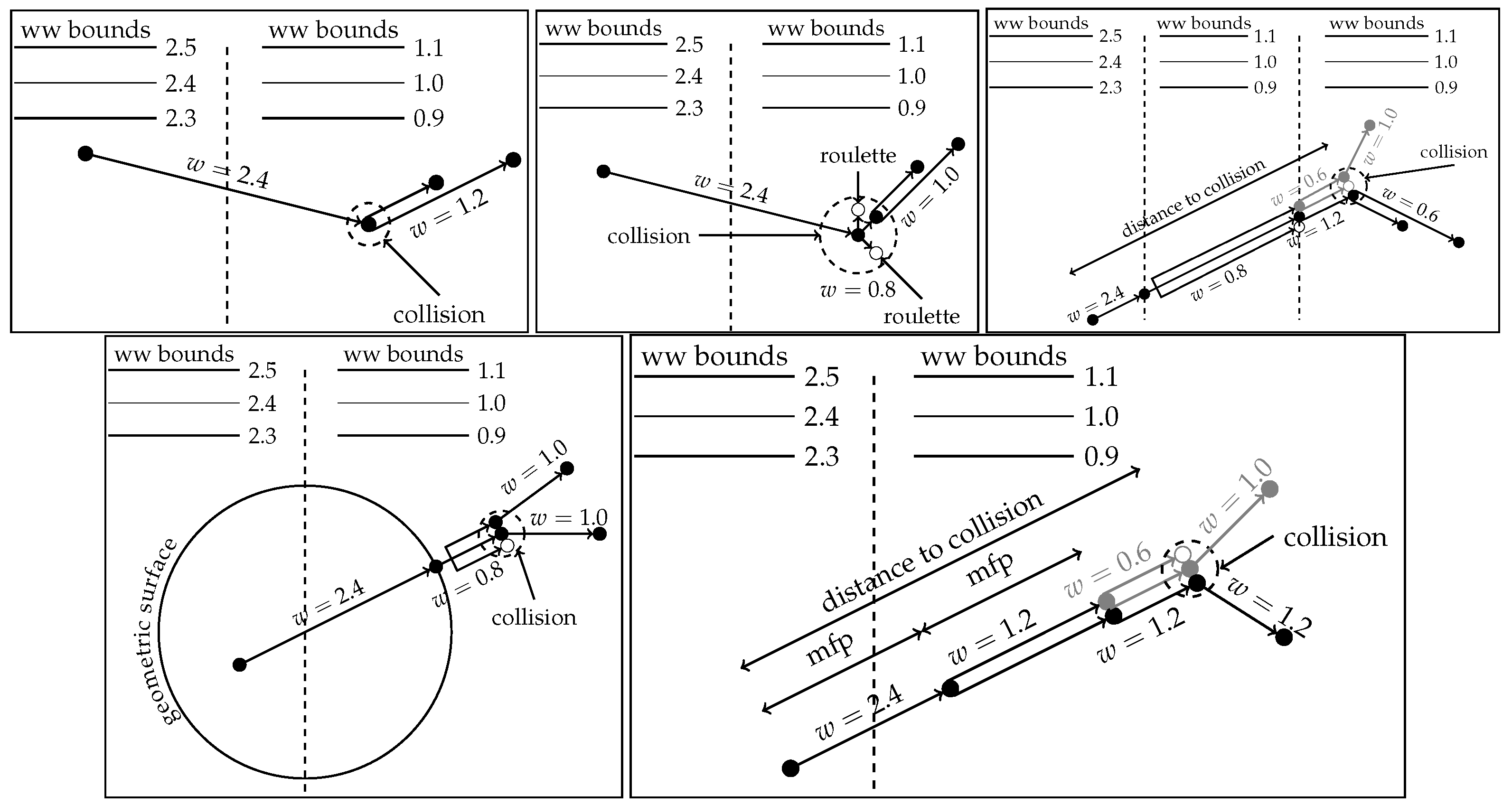
The remaining methods apply to traditional CADIS and FW-CADIS hybrid methods and are illustrated in Figure 1. The post_collision method performs a weight window lookup after a particle’s new post-collision direction and energy have been sampled and collision-related tallies have been scored. A simplified random walk with post-collision splitting/rouletting is depicted in Figure 1 (top left). All split particles begin their random walks from the same position, energy, and direction as the (post-collision) parent particle.
All of the methods discussed below perform post-collision weight window lookups in addition to lookups during other events. The rationale for this is that post-collision particles may be in a different window, and low-weight particles should be rouletted quickly to minimize the cost of transporting them. The pre_collision method performs weight window lookups both before and after a collision. If the particle is rouletted, then a potentially expensive scattering calculation is avoided, while splitting before sampling a new direction and energy results in a wider distribution of post-scatter directions and energies. To our knowledge, pre-collision weight window lookups are novel. An example random walk with pre-collision splitting/rouletting is depicted in Figure 1 (top center).
The tracking method performs weight window lookups after a weight window boundary has been crossed. This method requires simultaneous tracking through both the underlying model geometry and the weight window mesh. This additional tracking adds some computational burden to the calculation, especially on a fine importance mesh. This method is illustrated in Figure 1 (top right). This is the weight window lookup method used in MAVRIC. A similar method is the surface method, which performs weight window lookups after a geometric surface has been crossed. This method could be computationally expensive for geometries with a large number of surfaces per mean-free path. This method is illustrated in Figure 1 (bottom left).
Finally, the mfp method performs a weight window lookup every time a particle travels one mean-free path. This method is illustrated in Figure 1 (bottom right). This method requires a particle to carry its distance remaining until a mean-free path is reached, but does not require tracking on an additional mesh, as with the tracking method. Various permutations of these five initiating transport events were also studied. The mfp_precollision, mfp_surface, and mfp_surf_precol methods combine the individual mfp, surface, and pre_collision methods. The mfp, surface, and mfp_surface methods are all implemented in MCNP.
3. Results
The comparative performance of these methods was investigated using two different model problems: a small urban model and a spent fuel canister. In each model problem, all routines were evaluated on the basis of a figure of merit (FOM) [7]. While particle splitting reduces the variance, it increases the overall simulation runtime. Conversely, rouletting particles increases the solution variance but decreases the simulation runtime. Ultimately, the lowest variance for a runtime is sought. Therefore, the FOM is defined by
and is dependent on both the solution variance, , and total Monte Carlo simulation time, T. Larger FOM means lower run times for a given accuracy. In all simulations, the FW-CADIS method was used to generate the weight windows and source biasing. The cost of the deterministic calculations used to construct the weight windows and biased sources has been excluded from the computation of the FOM.
All of the following results were performed at ORNL on compute clusters featuring dual-processor AMD Opteron 6378 CPUs with 16 cores per CPU, for a total of 32 cores per node, and 128 GB RAM per node. All simulations were run on eight nodes (256 cores).
3.1. Urban Model
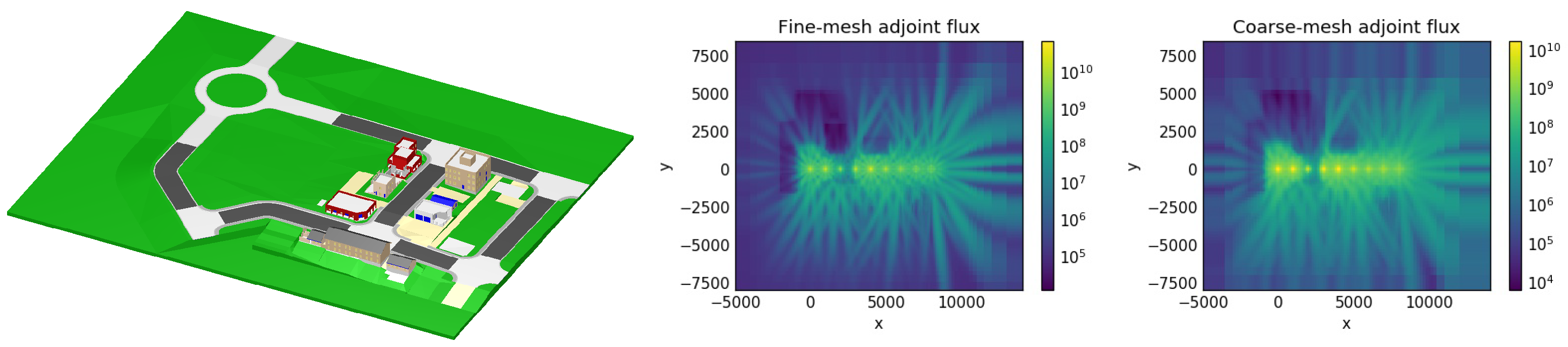
The splitting/rouletting routines were first tested on a Fort Indiantown Gap Combined Arms Collective Training Facility (CACTF) model. Background radiation sources are defined for all non-air materials in the model, and nine tallies were placed at 1 m intervals down the middle of the road that forms an urban canyon between buildings. This model is illustrated in Figure 2 (left). The model extends beyond what is shown in Figure 2 to capture the effect of skyshine. A sodium-iodide dose response function was applied to the detector tallies. Details of the model and the detector locations are found in Celik et al. [8].
The weight windows were generated with Denovo [9] using a fine (as fine as practical) and coarse mesh, using a 19-group ENDF-VII.1 photon shielding library, scattering, a 4 × 4 quadruple-range quadrature, and the step characteristics method. These parameters were chosen to expedite the calculation of weight windows and are not intended to necessarily produce ideal variance reduction parameters. Excluding regions distant from the buildings, in the x-axis the fine mesh contains 19 mesh planes between −3000 cm and −1000 cm, 199 mesh planes between −1000 cm and 9000 cm, and 14 mesh planes between 9000 cm and 10,500 cm. In the y-axis, the fine mesh contains 49 mesh planes between −6500 cm and −1500 cm, 59 mesh planes between −1500 cm and 1500 cm and 34 mesh planes between 1500 cm and 5000 cm. The fine mesh contains 39 mesh planes between −600 cm and 1400 cm in the z-axis. The coarse mesh contains half as many mesh cells in each direction as the fine mesh in the vicinity of the buildings. The problem domain extends well beyond these bounds to account for skyshine. All of the splitting/rouletting methods were run with Shift using ENDF-VII.1 continuous energy cross sections with particle histories. Solve time for the fine mesh Denovo solution was 167 s for both forward and adjoint, and 29 s and 30 s for the coarse mesh forward and adjoint solves, respectively. The analog Monte Carlo run took 5097 s.
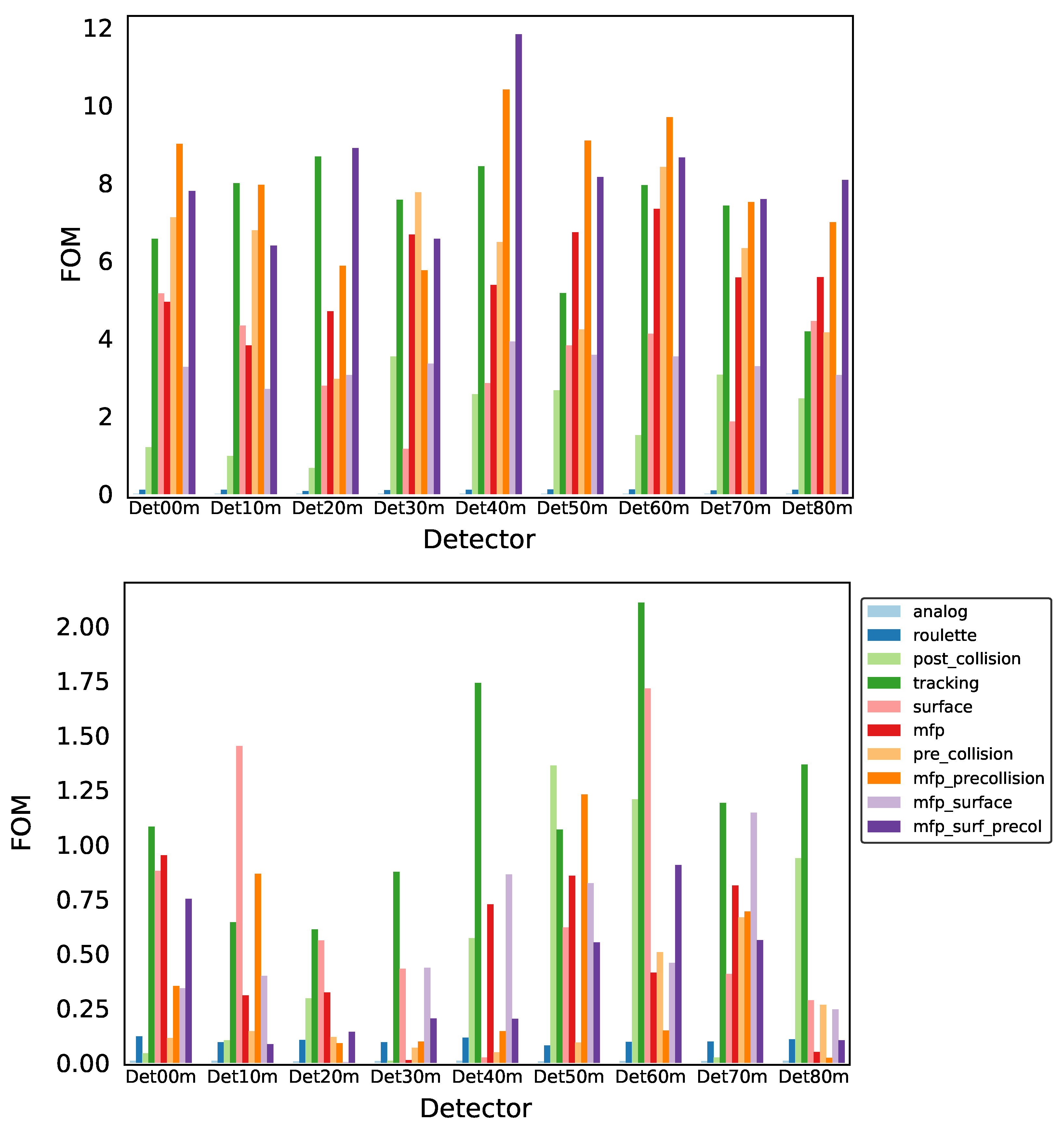
Figure 3 shows that the methods using a weight window mesh yield a gain of 3 to 4 orders of magnitude in the FOM compared to the roulette method (the analog FOM is very low and thus not resolved in the figure). For the fine mesh, methods combining the mfp and pre_collision methods most consistently yield the highest FOMs. The tracking method typically follows closely behind these methods in performance. The coarse mesh shows nearly an order of magnitude decrease in the FOMs when compared to the fine mesh. This is likely a result of the decreased accuracy of the adjoint solution on the coarse mesh. The coarse mesh results also show that the tracking method has the highest FOM. This is potentially due to the larger size of the weight windows allowing for multiple mean-free paths, collisions, and/or surface crossings to occur while a particle is within a single weight window. This would add computational time without reducing the variance of the solution. In all cases, post_collision performs relatively poorly. A diagnostic tool for tallying the location and frequency of splitting/rouletting events might prove useful for future analysis.
3.2. Spent Fuel Cask
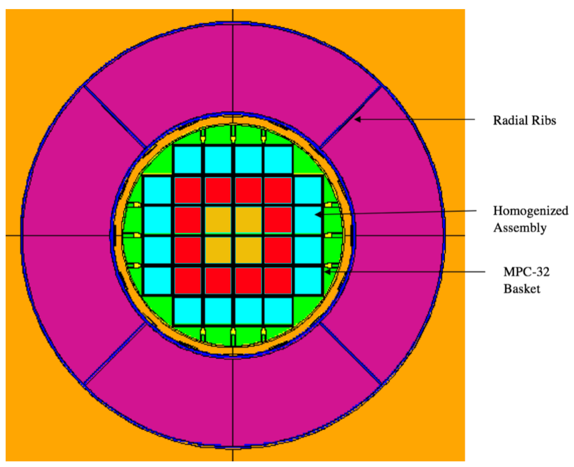
The weight window lookup methods were also tested on a spent fuel cask. This cask is an MCNP model of a Holtec International HI-STORM 100 spent nuclear fuel storage cask containing a multipurpose canister (MPC)-32 [10]. A Westinghouse 17 × 17 fuel assembly is used to model the fuel loading. The materials used for the cross sections in the active fuel region are modeled as homogeneous, fresh 3.71 wt% UO. Neutron source terms are calculated using the ORIGAMI sequence in SCALE [11] using a 10-node axial burnup profile for three different burnups. The burnups vary between the four inner assemblies, the 12 assemblies in the middle region, and 16 outer assemblies. The cross sectional geometry of the HI-STORM cask and source regions are shown in Figure 4. The burnups of the three source regions and the energy bins of the neutron source are shown in Table 1.
The canister is centered about the z-axis and extends from −62.23 cm to 582.295 cm, and has a radius of 166.37 cm. As with the urban model in Section 3.1, this problem was run with both fine and coarse weight window meshes. Along the x- and y-axis, the fine mesh has 24 uniform mesh planes between −600 cm and −200 cm, 149 uniform mesh planes between −200 cm and 200 cm, and 24 mesh planes between 200 cm and 600 cm. There are 99 uniform mesh planes in the axial z-direction between −62.23 cm and 600 cm. For the coarse mesh, the x- and y-axis each have 5 mesh planes between −600 cm and −200 cm, 49 mesh planes between −200 cm and 200 cm, and 5 mesh planes between 200 cm and 600 cm, with 49 mesh planes between −62.23 cm and 600 cm in the z-axis. The weight windows were built with Denovo using a 28-group ENDF-VII.1 cross section shielding library, step characteristics, a 4 × 4 quadruple-range quadrature, and scattering. Shift was run with 10 particles using continuous ENDF-VII.1 cross sections. The fine-mesh Denovo forward and adjoint solutions required 172 s and 211 s, respectively, while the coarse-mesh forward and adjoint solutions took 44 s and 36 s, respectively. The analog Monte Carlo run required 2231 s.
A mesh tally was used that spanned −500 cm to 500 cm divided by 19 mesh planes in the x- and y-directions, and spanned −62.23 cm to 600 cm divided by two mesh planes in the z-direction. A tissue dose response function was applied to the tally. There are many ways to average the variance over a mesh tally for computing the FOM. In this work, we simply average the variance over the tally volume.
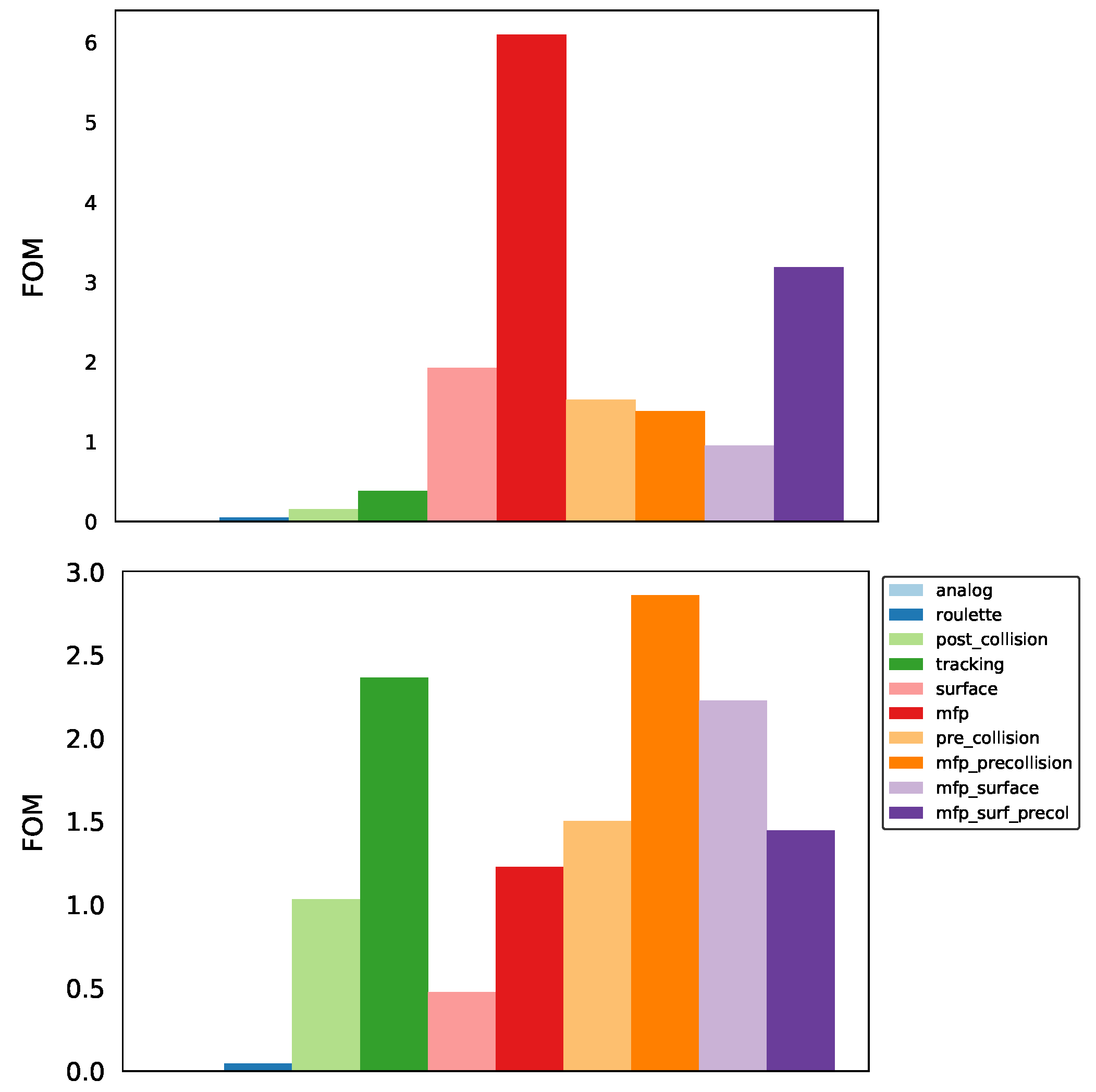
Results are shown in Figure 5. The analog FOM is very low and not resolved in the figure. When running with a fine weight window mesh, the mfp weight window lookup method outperformed all others by a wide margin. This is somewhat in contrast with the results presented in Section 3.1, in which mfp alone did not perform as well as when combined with precollision and surface. The reason that mfp performs so well while mfp_surf_precol and especially mfp_surface do not is not immediately clear. One possible explanation is that the mean-free path through the cask is small enough that adding additional lookups during each geometric crossing adds computational expense without adding value. For the coarse mesh result, it was found that tracking performs very well, as was the case with the coarse mesh results in Section 3.1. In this case the performance of tracking was slightly exceeded by the performance of mfp_precollision.
4. Conclusions
Some overarching observations can be drawn from this study. Foremost, as expected, finer weight window meshes produce higher FOMs than coarser meshes. The tracking method performs well for problems using a coarse weight window mesh, which may be the result of avoiding multiple weight window lookups while a particle is within a single mesh element, althought it is not always the best performing method. Note also that the performance of the tracking method is dependent upon the geometry of the weight window mesh. Storing weight windows on more complex geometries (such as block-structured grids [12]) will make the tracking method more computationally expensive relative to other methods.
Less clear is the best method when using a fine weight window mesh, although methods employing pre_collision frequently perform well. This is not unexpected, since the pre_collision method allows for a wider distribution of particle directions and energies from a collision, thus distributing particles more uniformly throughout phase space. Adding lookups every mean-free path and geometric surface crossing usually improves the method. It was also found that using post_collision splitting/rouletting alone did not perform well regardless of the weight window grid.
A diagnostic tool for tallying locations of splitting/rouletting might help explain the FOM performance for various weight window lookup methods. Additional parameters, such as the quadrature order used by the deterministic adjoint solver, or further refinement of the weight window mesh could also be studied. Additional permutations of the weight window lookup methods could also be added in future studies.
Author Contributions
Conceptualization, G.G.D.; methodology, G.G.D.; software, E.S.G. and G.G.D.; validation, G.G.D.; formal analysis, E.S.G. and G.G.D.; investigation, E.S.G. and G.G.D.; resources, G.G.D.; data curation, E.S.G. and G.G.D.; writing—original draft preparation, E.S.G.; writing—review and editing, G.G.D.; visualization, E.S.G. and G.G.D.; supervision, G.G.D.; project administration, G.G.D.; funding acquisition, G.G.D. All authors have read and agreed to the published version of the manuscript.
Funding
Work for this paper was supported by ORNL, which is managed and operated by UT-Battelle LLC, for the US Department of Energy under Contract No. DEAC05-00OR22725. This work was sponsored by the US Nuclear Regulatory Commission under task order NRC-HQ-60-17-T-0027 and was performed under the Nuclear Engineering Science Laboratory Synthesis (NESLS) program at ORNL. This work was also sponsored by the Enabling Capabilities for Nonproliferation and Arms Control Program Area of the Office of Defense Nuclear Nonproliferation Research and Development, National Nuclear Security Administration.
Conflicts of Interest
The authors declare no conflict of interest.
References
- Wagner, J.C.; Haghighat, A. Automated Variance Reduction of Monte Carlo Shielding Calculations Using the Discrete Ordinates Adjoint Function. Nucl. Sci. Eng. 1998, 128, 186–208. [Google Scholar] [CrossRef]
- Wagner, J.C.; Peplow, D.E.; Mosher, S.W. FW-CADIS Method for Global and Regional Variance Reduction of Monte Carlo Radiation Transport Calculations. Nucl. Sci. Eng. 2014, 176, 37–57. [Google Scholar] [CrossRef]
- Peplow, D.E. Monte Carlo Shielding Analysis Capabilities with MAVRIC. Nucl. Technol. 2011, 174, 289–313. [Google Scholar] [CrossRef]
- Thompson, W.L.; Deutsch, O.L.; Booth, T.E. Deep Penetration Calculations; Technical Report ORNL/RSIC-44; Oak Ridge National Laboratory: Oak Ridge, TN, USA, 1980. [Google Scholar]
- X.M.C. Team. MCNP—A General Monte Carlo N-Particle Transport Code, Version 5; Technical Report LA-UR-03-1987; Los Alamos National Laboratory: Los Alamos, NM, USA, 2008. [Google Scholar]
- Pandya, T.M.; Johnson, S.R.; Evans, T.M.; Davidson, G.G.; Hamilton, S.P.; Godfrey, A.T. Implementation, Capabilities, and Benchmarking of Shift, a Massively Parallel Monte Carlo Radiation Transport Code. J. Comput. Phys. 2016, 308, 239–272. [Google Scholar] [CrossRef] [Green Version]
- Briesmeister, J. MCNP—A General Monte Carlo N-Particle Transport Code, Version 4C; Technical Report LA-13709-M; Los Alamos National Laboratory: Los Alamos, NM, USA, 1993. [Google Scholar]
- Celik, C.; Peplow, D.E.; Davidson, G.G.; Swinney, M.W. A Directional Detector Response Function for Anisotropic Detectors. Nucl. Sci. Eng. 2019, 193, 1355–1370. [Google Scholar] [CrossRef]
- Evans, T.M.; Stafford, A.S.; Slaybaugh, R.; Clarno, K.T. Denovo: A new three-dimensional parallel discrete ordinates code in SCALE. Nucl. Technol. 2010, 171, 171–200. [Google Scholar] [CrossRef]
- Final Safety Analysis Report for the HI-STORM 100 CASK System Rev. 9; Holtec International: Marlton, NJ, USA, 2010.
- Rearden, B.T.; Jessee, M.A. (Eds.) SCALE Code System; Number ORNL/TM-2005/39, Version 6.2; Oak Ridge National Laboratory: Oak Ridge, TN, USA, 2016. [Google Scholar]
- Flaspoehler, T.; Petrovic, B. Contributon-Based Mesh-Reduction Methodology for Hybrid Deterministic-Stochastic Particle Transport Simulations Using Block-Structured Grids. Nucl. Sci. Eng. 2018, 192, 254–274. [Google Scholar] [CrossRef]
Figure 1.
A selection of weight window lookup events being studied: post-collision (top left), pre-collision (top center), tracking (top right), surface crossing (bottom left), and mfp (bottom right). In this figure, post-collision particles are assumed to occupy a higher importance region.
Figure 1.
A selection of weight window lookup events being studied: post-collision (top left), pre-collision (top center), tracking (top right), surface crossing (bottom left), and mfp (bottom right). In this figure, post-collision particles are assumed to occupy a higher importance region.

Figure 2.
Urban CACTF model (left), total adjoint flux for the fine mesh (center) and total adjoint flux for the coarse mesh (right). Photon detectors are placed in various locations along the road that passes between the buildings.
Figure 2.
Urban CACTF model (left), total adjoint flux for the fine mesh (center) and total adjoint flux for the coarse mesh (right). Photon detectors are placed in various locations along the road that passes between the buildings.

Figure 3.
FOM comparison for weight window lookup methods on the urban model with the fine weight window mesh (top) and coarse weight window mesh (bottom).
Figure 3.
FOM comparison for weight window lookup methods on the urban model with the fine weight window mesh (top) and coarse weight window mesh (bottom).

Figure 4.
Cross section of HI-STORM 100 SNF storage cask. The inner source region is shown in yellow, the middle source region is red, and the outer source region is blue.
Figure 4.
Cross section of HI-STORM 100 SNF storage cask. The inner source region is shown in yellow, the middle source region is red, and the outer source region is blue.

Figure 5.
FOM comparison for weight window lookup methods on the spent fuel cask with neutron dose for fine mesh weight windows (top) and coarse mesh weight windows (bottom).
Figure 5.
FOM comparison for weight window lookup methods on the spent fuel cask with neutron dose for fine mesh weight windows (top) and coarse mesh weight windows (bottom).


Table 1.
Burnup for the three source regions (left) and source energy bins (right).
| Region | Burnup | Enrichment | Cooling Time | Neutron Energy Bins | |
|---|---|---|---|---|---|
| (Gwd/MtU) | (wt%) | (yr) | (MeV) | ||
| Inner | 60 | 5 | 12 | 0.1–0.4 | |
| Middle | 50 | 4.8 | 10 | 0.4–0.9 | |
| Outer | 45 | 4.8 | 10 | 0.9–1.4 | |
| 1.4–1.85 | |||||
| 1.85–3.0 | |||||
| 3.0–6.43 | |||||
| 6.43–20.0 |
Publisher’s Note: MDPI stays neutral with regard to jurisdictional claims in published maps and institutional affiliations. |
© 2021 by the authors. Licensee MDPI, Basel, Switzerland. This article is an open access article distributed under the terms and conditions of the Creative Commons Attribution (CC BY) license (http://creativecommons.org/licenses/by/4.0/).
Share and Cite
MDPI and ACS Style
Gonzalez, E.S.; Davidson, G.G. Choosing Transport Events for Initiating Splitting and Rouletting. J. Nucl. Eng. 2021, 2, 97-104. https://0-doi-org.brum.beds.ac.uk/10.3390/jne2020010
AMA Style
Gonzalez ES, Davidson GG. Choosing Transport Events for Initiating Splitting and Rouletting. Journal of Nuclear Engineering. 2021; 2(2):97-104. https://0-doi-org.brum.beds.ac.uk/10.3390/jne2020010
Chicago/Turabian StyleGonzalez, Evan S., and Gregory G. Davidson. 2021. "Choosing Transport Events for Initiating Splitting and Rouletting" Journal of Nuclear Engineering 2, no. 2: 97-104. https://0-doi-org.brum.beds.ac.uk/10.3390/jne2020010