
Proximal Policy Optimization for Radiation Source Search


1
Department of Electrical and Computer Engineering, Portland State University, Portland, OR 97201, USA
2
Department of Nuclear Engineering, University of New Mexico, Albuquerque, NM 87131, USA
3
Center for High Technology Materials, University of New Mexico, 1303 Goddard St SE, Albuquerque, NM 87106-4343, USA
*
Author to whom correspondence should be addressed.
J. Nucl. Eng. 2021, 2(4), 368-397; https://0-doi-org.brum.beds.ac.uk/10.3390/jne2040029
Submission received: 29 July 2021
/
Revised: 17 September 2021
/
Accepted: 26 September 2021
/
Published: 30 September 2021
(This article belongs to the Special Issue Nuclear Security and Nonproliferation Research and Development)
Abstract
:Rapid search and localization for nuclear sources can be an important aspect in preventing human harm from illicit material in dirty bombs or from contamination. In the case of a single mobile radiation detector, there are numerous challenges to overcome such as weak source intensity, multiple sources, background radiation, and the presence of obstructions, i.e., a non-convex environment. In this work, we investigate the sequential decision making capability of deep reinforcement learning in the nuclear source search context. A novel neural network architecture (RAD-A2C) based on the advantage actor critic (A2C) framework and a particle filter gated recurrent unit for localization is proposed. Performance is studied in a randomized m convex and non-convex simulation environment across a range of signal-to-noise ratio (SNR)s for a single detector and single source. RAD-A2C performance is compared to both an information-driven controller that uses a bootstrap particle filter and to a gradient search (GS) algorithm. We find that the RAD-A2C has comparable performance to the information-driven controller across SNR in a convex environment. The RAD-A2C far outperforms the GS algorithm in the non-convex environment with greater than median completion rate for up to seven obstructions.
1. Introduction
The advancement of nuclear technology has brought the benefits of energy production and medical applications, but also the risks associated with exposure to radiation [1]. Radioactive materials can be used for dirty bombs, or might be diverted from its intended use. Effective detection when these types of materials are present in the environment is of the utmost importance and measures need to be in place to rapidly locate a source of radiation in an exposure event to limit human harm [2]. Autonomous search methods provide a means of limiting radiation exposure to human surveyors and can process a larger array of information than humans to inform the search strategy. Additionally, these techniques can operate in environments where limited radio communication would prevent untethered remote-control of a robot such as the Fukushima Daiichi disaster [3].
Detection, localization, and identification are based upon the measured gamma-ray spectrum from a radiation detector. Radioactive sources decay at a certain rate which, with the amount of material, gives an activity, often measured in disintegrations per second or becquerels [bq]. Most decays leave the resulting nucleus in an excited state, which may lose energy by emitting specific gamma rays. With decay branching, not all decays might emit one gamma ray, so to remove ambiguity, we look at the gamma rays emitted per second [gps] instead of decays per second. Localization methods in the current work rely upon the intensity in counts per second [cps] of the gamma photon radiation measured by a single, mobile scintillation detector that is searching for the source and is composed of a material such as sodium iodide (NaI) [4]. Other localization techniques such as coded mask aperture imaging or Compton imaging are also effective but are not applicable in the case of a non-convex environment. The number of counts per second recorded by a detector is related to the total photons emitted per second through a scaling factor determined by detector characteristics. It is common to approximate each detector measurement as being drawn from a Poisson distribution because the success probability of each count is small and constant [4]. The size of the detector also affects count rates, with a larger detector having a larger solid angle. The inverse square relationship, , is a useful approximation to describe the measured intensity of the radiation as a function of the distance between the detector and source, d. This nonlinear relationship paired with the probabilistic nature of gamma-ray emission and background radiation from the environment leads to ambiguity in the estimation of a source’s location.
In the case of a single mobile detector, there are numerous challenges to overcome. Detectors deployed to smaller autonomous systems such as drones or robots have a smaller surface area and volume resulting in poorer counting statistics per dwell time. Common terrestrial materials such as soil and granite contain naturally occurring radioactive materials that can contribute to a spatially varying background rate [4]. Far distances, shielding with materials such as lead, and the presence of obstructions, can significantly attenuate or block the signal from a radioactive source. We will refer to environments with obstructions as being non-convex, in line with the notion of convexity in set theory [5]. Further challenges arise with multiple or weak sources. Given the high variation in these variables, the development of a generalizable algorithm with minimal priors becomes quite difficult. Additionally, algorithms for localization and search need to be computationally efficient due to energy and time constraints. Figure 1 shows an example illustration of a mobile robot performing active nuclear source search in a non-convex environment.
1.1. Machine Learning (ML)
ML is broadly concerned with the paradigm of computers learning how to complete tasks from data. Reinforcement learning (RL) is a subset of ML focused on developing a control policy that maximizes cumulative reward in an environment. Deep learning (DL) is another subset of ML with an emphasis on approximating a function of interest using a dataset and compositions of elementary linear and nonlinear functions. These function compositions can be stacked in succession to create “layers”, thereby increasing the complexity of functions of interest that can be approximated, and giving rise to the term “deep” in DL. A key difference between RL and other subsets of ML is the process of data acquisition. Learning in RL is dependent on data that is collected while the policy is acting in the environment, thereby having a direct impact on the data collected in the future. The majority of other ML techniques utilize datasets acquired before training. The intersection of RL and DL has resulted in a framework called Deep reinforcement learning (DRL). DRL uses deep neural networks to learn a control policy and approximate state values through trial and error in an environment. While training of these networks is computationally intensive, once the weights are learned, inference (the application of a trained ML model) can be performed at lower computational cost. In this paper, we investigate a branch of DRL known as stochastic, model-free, on-policy gradients and assess its performance in the task of control in the radiation source search domain.
DRL has far surpassed human expertise in a myriad of other tasks, for example, the board game Go, which has a state space of [6]. Since these algorithms learn strictly through environmental interaction, they can discover and develop heuristics and action trajectories that humans might never have considered in their algorithm design. Radiation source search is a well studied problem, and there are many solutions provided certain assumptions hold such as known background rate or environment layout. Data-driven approaches have received less attention, in part, because of the high variability of enivornmental parameters mentioned above. This paper demonstrates that DRL can learn an effective policy that generalizes across a range of scenarios where background rate, source strength and location, and the number of obstructions are varied.
1.2. Related Work
Many solutions have been proposed for nuclear source search and localization across a broad range of scenarios and radiation sensor modalities. These methods are generally limited to the assumptions made about the problem such as the background rate, mobility of the source, shielding presence, and knowledge of obstruction layout and composition. Morelande et al. present a maximum likelihood estimation approach and a Bayesian approach to multi-source localization using multiple fixed detectors in an unobstructed environment [7]. Hite et al. also use a Bayesian approach with Markov chain Monte Carlo to localize a single point source in a cluttered urban environment by modeling the radiation attenuation properties of different materials [8]. Hellfeld et al. focused on a single detector in 3D space moving along a pre-defined path for single and multiple weak sources [9]. They utilized an optimization framework with sparsity regularization to estimate the source activity and coordinates.
There is great interest in autonomous search capabilities for source search to limit human exposure to harmful radiation. Cortez et al. proposed and experimentally tested a robot that used variable velocity uniform search in a single source scenario [10]. Ristic et al. proposed three different formulations of information-driven search with Bayesian estimation. An information-driven search algorithm selects actions that maximize the available information for its estimates of user-specified quantities at each timestep. The first method utilized a particle filter (Appendix B.1) and the Fisher information matrix (Appendix B.2) for a single source and single detector in an open area with constant background [11]. The second and third method both used the Renyi information divergence metric (Appendix B.3) and particle filter to control a detector/detectors in convex/non-convex environments with multiple sources, respectively [12,13]. In the non-convex environment, the layout was considered to be known before the start of the search. Anderson et al. considered a single mobile detector used for locating multiple sources in a non-convex environment through an optimization based on the Fisher information and travel costs [14]. The obstruction attenuation and nuclear decay models were specified by hand.
RL and DRL have also been applied to the control of single robots. Landgren used a multi-armed bandit approach to control nuclear source search in an indoor environment [15]. This was implemented on a Turtlebot3 and used to find multiple radioactive sources in a lab through radiation field sampling. Liu et al. used double Q-learning to control a single detector search for a single radioactive source with a varying sized wall in simulation [16]. The model performed well when the test environment matched its training set but did not generalize when new geometries were introduced and had to be retrained. This approach is the most similar to the one used in this research.
In contrast to the majority of the methods mentioned above, our algorithm does not directly rely on any hard-coded modeling assumptions for decision making. This gives greater flexibility to our approach and allows the opportunity for generalization to a greater variety of situations. For example, our approach was only trained on up to five obstructions in an environment at any one time but can easily operate when greater than five obstructions are present. Additionally, it would be relatively simple to retrain the agent to account for a moving source or novel obstruction types and layouts, among other things. This comes with the caveat that there is a heavy reliance upon the assumptions made in modeling an environment that are likely to fail in capturing the intricacies of reality (reality gap). This is an area of intense interest in the DRL research space [17].
1.3. Contributions
The main contributions of this paper are an on-policy, model-free DRL approach to radiation source search, a novel neural network architecture, the RAD-A2C, and an open-source radiation simulation for convex and non-convex environments. Our approach will be evaluated in the context of single detector search for a single radiation source in a simulated 2D environment with variable background radiation, variable source intensity and location, variable detector starting position, and variable number of obstructions. The RAD-A2C will be compared against a modified information-driven search algorithm previously proposed in the nuclear source search literature and a gradient search algorithm in a convex environment across signal-to-noise ratio (SNR)s. We will examine the effect of obstructions on the RAD-A2C performance in a non-convex environment with comparison to a gradient search algorithm across SNRs.
2. Materials and Methods
2.1. Radiation Source Search Environment
The radiation source search environment was fundamental to the training of the policy. The development of the environment required many careful design decisions in an attempt to provide a useful proof of concept for the efficacy of DRL in practical radiation source search contexts. In the remainder of the paper, we assume that a gamma radiation source has already been detected through some other means and the objective is to now locate it. We also assume an isotropic detector and a constant background rate per environment. An episode is defined to be a finite sequence (successfully completed or the maximum number of timesteps was reached) of observations, actions, and rewards in an environment.
2.1.1. Partial Observability
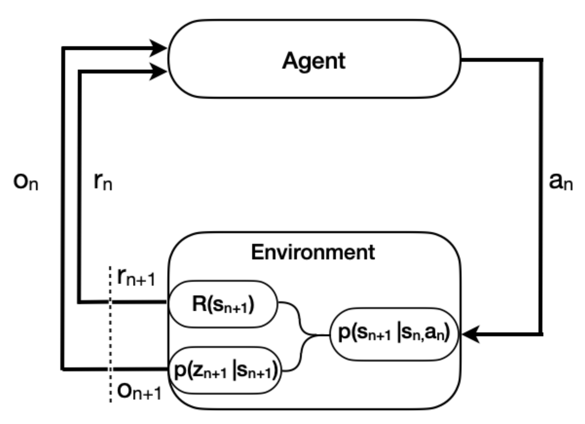
In the context of the radiation search scenario where measurements are noisy and uncertain, it is useful to describe the partially observable Markov decision process (POMDP). The finite POMDP is defined by the 6-tuple at each time step, n. are the finite sets of states, state measurements, actions, and rewards, respectively. A state, , corresponds to all the components of the environment, some fully observable such as the detector location and range sensor measurements, and others, hidden, such as source activity and source location. A state measurement, , is the detector’s measurement of the radiation source governed by the state measurement probability distribution, , equivalent to Equation (3). A state measurement is a function of the true state but is not necessarily representative of the true state due to the stochastic nature of the environment. An action, , determines the direction the detector will be moved. The reward, , corresponds to a scalar value determined by the reward function defined in Equation (4). The state transition density, , is unity in our context as the state components only change deterministically. An observation, , denotes the vector containing the fully observable components of the state and state measurement . Figure 2 shows the POMDP for an episode consisting of the observation, action, reward loop that continues until the episode termination criteria is met.
A history is a sequence of observations up to timestep n, that is defined as . A successful policy needs to consider to inform its decisions since a single observation does not necessarily uniquely identify the current state. This can be implemented directly by concatenation of all previous observations with the current observation input or through the use of the hidden state, , of a recurrent neural network (RNN). The sufficient statistic is a function of the past history and serves as the basis for the agent’s decision making [18]. In this work, , where denotes a RNN parameterization. This allows the control policy to be conditioned on as , where p is some probability distribution, is some neural network parameterization, and is the next action. Our parameterization was a two layer perceptron with hyperbolic tangent activation functions after the first layer only. The distribution p was selected to be multinomial as the set of actions was discrete. A Gaussian distribution can be used in the case of a continuous action space.
2.1.2. Gamma Radiation Model
Gamma radiation measured by a detector typically comes in two configurations, the total gamma-ray counts or the gamma-ray counts in specific peaks. The full spectrum is more information rich as radiation sources have identifiable photo-peaks but is more complex and computationally expensive to simulate. Thus, our localization and search approach uses the gross counts across the energy bins. Cesium-137 was selected as the source of interest since it is commonly used in industry applications and is fairly monoenergetic [19]. As we are not performing spectroscopic discrimination, our value to describe source intensity is just gamma rays emitted per second [gps] with the generous assumption of detector efficiency across the spectrum. We denote the parameter vector of interest as , where are the source coordinates in [m]. These quantities are assumed to be fixed for the duration of an episode. An observation at each timestep, n, is denoted as , and consists of the measured counts, , detector position denoted , and 8 obstruction range sensor measurements for each direction of detector movement. This modeled some range sensing modality such as an ultrasonic or optical sensor. The maximum range was selected to be m to allow the controller to sense obstructions within its movement step size. The range measurements were normalized to the interval , where 0 corresponds to no obstruction within range of the detector and 1 corresponds to the detector in contact with an obstruction.
The background radiation rate is a constant [cps] as seen by the detector. The following model is used to approximate the mean rate of radiation counts measurements in an unobstructed environment (convex),
where A, , and , are the detector cross sectional area area, the detector intrinsic efficiency, and the dwell time [s], respectively. The detector intrinsic efficiency is assumed to be one and we consider a unit dwell time. The calculations are performed using centimeters, and the detector is assumed to be a cylinder with area equal to [cm] with an isotropic response for ease of computation. This results in the following binary attenuation model when the detector’s line-of-sight (LOS) is or is not blocked by an obstruction:
Thus, the measurement likelihood function is defined as
2.1.3. Reward Function
The reward function defines the objective of the DRL algorithm and completely determines what will be learned from the environment. Reward is only utilized for the update of the weights during the optimization phase and does not directly factor into the DRL agent’s decision making during an episode. The reward function for the convex and non-convex environment is as follows,
Here, the source-detector shortest path distance is defined as , and defines the largest Euclidean distance between vertices of the search area. The shortest path distance is essential for the non-convex environment and becomes the Euclidean distance when there is LOS due to the visibility graph implementation. The normalization factor, , in the negative reward provides an implicit boundary to the search area. This reward scheme incentivizes the DRL agent to find the source in the fewest actions possible as the negative reward is weighted more heavily. The reward magnitudes were selected so that standardization was not necessary during the training process as mean shifting of the reward can adversely affect training [21].
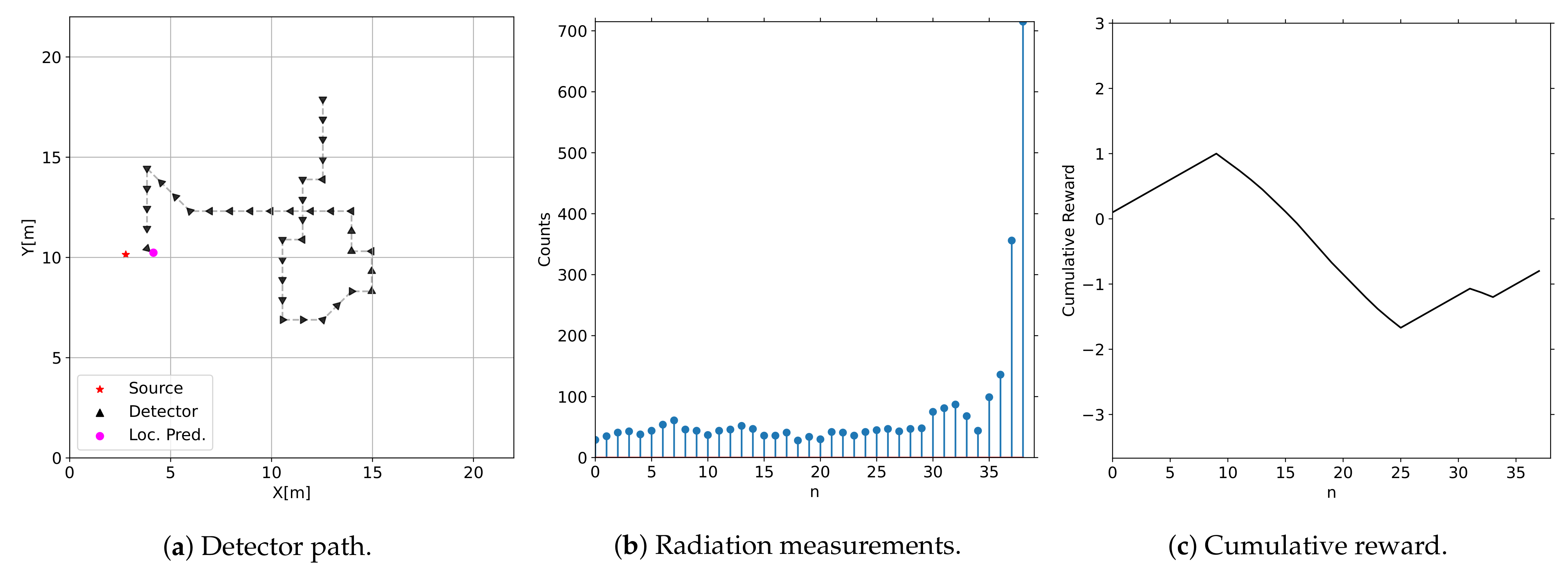
The reward function was designed to provide greater feedback for the quality of an action selected by the DRL agent in contrast to only constant rewards. For example, in the negative reward case, if the DRL agent initially takes actions that increase above the previous closest distance for several timesteps and then starts taking actions that reduce , the negative reward will be reduced as it has started taking more productive actions. This distance-based reward function gives the DRL agent a more informative reward signal per episode during the learning process. Figure 4 shows an episode of the DRL agent operating within the environment, the radiation measurements it observes, and the reward signal it receives.
2.1.4. Configuration
Detector step size was fixed at 1 m/sample and the movement direction in radians was limited to the set, . The DRL implementation can easily be adapted to handle more discrete directions and variable step sizes or even continuous versions of these quantities. These two constraints were made to limit the computational requirements for the comparison algorithm. Maximum episode length was set at 120 samples to ensure ample opportunity for the policy to explore the environment, especially in the non-convex case. Episodes were considered completed if the detector came within m of the source or a failure if the number of samples reached the maximum episode length. The termination distance was selected to cover a range of closest approaches as the detector movement directions and step size are fixed. The state space has eleven dimensions that include eight detector-obstruction range measurements for each movement direction, the radiation measurement, and the detector coordinates. If the policy selected an action that moved the detector within the boundaries of an obstruction, then the detector location was unchanged for that sample. Table 1 shows the parameters used for the environment simulation.
2.2. Reinforcement Learning (RL)
2.2.1. Background
The aim of RL is to maximize the expectation of cumulative reward over an episode through a policy learned by interaction with the environment. In this work, the policy, , is a stochastic mapping from states to actions that does not rely on estimates of the state value as required in methods such as Q-learning. We consider radiation source search to be an episodic task which dictates that the episodes are finite and that the environment and agent are reset according to some initial state distribution after episode completion. The cumulative reward starting from any arbitrary time index is defined as,
where N is the length of the episode and is the discount factor. This definition gives clear reward attribution for actions at certain timesteps and the total episode reward results when . The expected return of a policy over a collection of histories is then defined as,
where denotes the cumulative reward for a history H and is the probability of a history occurring given a policy.
The agent learns a policy from the environment reward signal by updating its value functions. The value function, , estimates the reward attainable from a given hidden state that gives the agent a notion of the quality of its hidden state [22]. This is also a means of judging the quality of a policy, as the value is defined as the expected cumulative reward across the episode when starting from hidden state and acting according to policy thereafter or more succinctly,
The temporal difference (TD) error is a method of generating update targets for the value function from experiences in the environment [23]. The TD error is defined using the value function as,
If a value function approximator is correctly predicting the value of a hidden state, then the TD error should be close to 0. Otherwise, the value function approximation must be updated to minimize this error. Prior to the application of DL to RL, policies and value functions took the form of lookup tables or other function approximations such as tile coding [22].
On policy, model-free DRL methods require that the agent learns a policy from its episodic experiences throughout training, whereas model-based methods focus on using a learned or given model to plan action selection. On policy methods are worse in terms of sample efficiency than Q-learning because the learning takes place in an episodic fashion, i.e., the policy is updated on a set of episodes and these episodes are then discarded. The benefit being that the agent directly optimizes policy parameters through the maximization of the reward signal. The decision to use model-free policy gradients was motivated by the stability and ease of hyperparameter tuning during training. Specifically, we used a variant of the advantage actor-critic (A2C) framework called PPO.
2.2.2. Proximal Policy Optimization (PPO)
The actor, , and critic, , are the two main components of the A2C where denote separate neural network parameterizations. The critic approximates the value function, , by regressing the hidden state onto a cumulative reward prediction. We also use an RNN, parameterized by , to encode the observations over time in the hidden state, , as specified in Section 2.1.1. The actor serves as the policy and at each timestep, calculates a distribution over actions defined as,
where and are the matrix of neural network weights and a vector of biases for the actor, respectively. The is the softmax function that transforms the network outputs to the interval and multi(·) is the multinomial distribution. The critic is utilized in the policy weight update as an approximation to the value function.
Schulman et al. propose the following generalized advantage estimator (GAE) with parameters to control the bias-variance tradeoff,
where is the TD error as defined in Equation (8). This is an exponentially-weighted average of the temporal differences error where determines the scaling of the value function that adds bias when and that adds bias when if the value function is inaccurate [24]. The weights for the policy are updated by taking the gradient of Equation (6) yielding,
A common issue in policy gradient methods is the divergence or collapse of policy performance after a parameter update step. This can prevent the policy from ever converging to the desired behavior or result in high sample inefficiency as the policy rectifies the performance decrease. Schulman et al. proposed the PPO algorithm as a principled optimization procedure to ensure that each parameter update stays within a trust-region of the previous parameter iterate [25]. We chose to use the PPO-Clip implementation of the trust-region because of the strong performance across a variety of tasks, stability, and ease of hyperparameter tuning as shown in [25,26].
The PPO-Clip objective is formulated as,
where k denotes the epoch index and is implicit in the hidden state. Here, , denotes the probability ratio of the previous policy iterate to the proposed policy iterate and is the clipping parameter that enforces a hard bound on how much the latest policy iterate can change in probability space reducing the chance of a detrimental policy update. A further regularization trick is early-stopping based on the approximate Kullback-Leibler divergence. The approximate Kullback-Leibler divergence is a measure of the difference between two probability distributions and the approximation is the inverse of in log space. If the approximate Kullback-Leibler divergence between the current and previous iterate over a batch of histories exceeds a user-defined threshold, then the parameter updates over that batch of histories are skipped.
The value function network parameters are updated on the mean square error (MSE) loss between the value function estimate and the empirical returns,
The total loss is then defined as
where c is a weighting parameter. Gradient ascent is performed on this loss to find the set of network parameters that maximize the expected episode cumulative reward.
2.3. RAD-A2C
2.3.1. Gated Recurrent Unit (GRU)
The GRU architecture proposed by Cho et al. is a subset of the recurrent neural network (RNN)s family that use gates to address the vanishing and exploding gradients encountered when using backpropagation-through-time and increase the network’s ability to establish dependencies across long temporal gaps [27]. The following set of equations describe the GRU operations,
where is the sigmoid activation function, is the bias term associated with each weight matrix, is the hyperbolic tangent activation function, denotes vector concatenation, and ⊙ is the Hadamard product. The GRU has more parameters than the standard RNN but the gain is in training stability and the increased range for sequence relationships.
Figure 5 shows the design of a single GRU cell recreated from Olah [28]. Each box represents a weight matrix and activation function and the circles represent mathematical operations. The conjoining lines represent the concatenation of the quantity and diverging lines represent the copying. The crux of the reset () and update () gates are to modify the candidate hidden state (), which then becomes the output hidden state (). The reset gate determines how much of the previous hidden state to factor into the new hidden state and the update gate determines the convex combination of the previous hidden state and the candidate hidden state. This cell is a drop-in replacement for the hidden state found in Figure 5a.
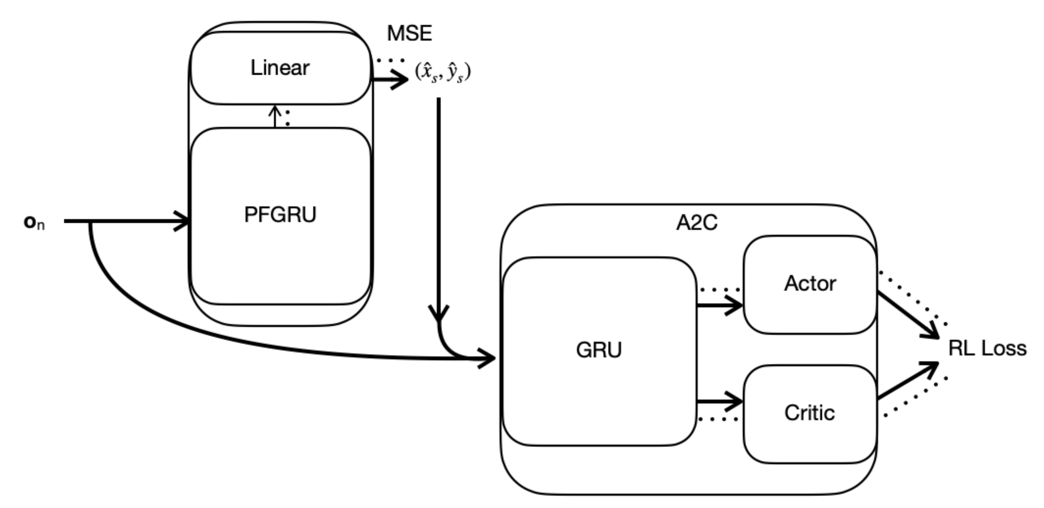
2.3.2. Architecture
The RAD-A2C is composed of a particle filter gated recurrent unit (PFGRU) proposed by Ma et. al [29] (Appendix A.1), one GRU module to encode the observations over time for action selection, and three linear layers. The model was implemented using the PyTorch library [30]. At each timestep, the observation is propagated to both the PFGRU and the A2C modules. The PFGRU uses a linear layer to regress its mean “particles” onto a source location, which is concatenated with the observation and fed into the A2C. The Actor layer regresses the GRU hidden state onto a multinomial distribution over actions using a softmax function. The Critic layer regresses the hidden state onto a value prediction. This value prediction is only necessary for the training phase and has no direct impact during inference. Figure 6 shows the RAD-A2C architecture and the flow of information through the system. The dotted lines indicate the path of the error gradients for backpropagation during training. Appendix A.2 covers implementation and training details and Table A1 shows the selected hyperparameters. The code is available at https://github.com/peproctor/radiation_ppo last accessed on 27 September 2021.
The RAD-A2C is easily extendible to other source search scenarios such as a 3D environment, moving sources, using more advanced radiation transport simulators, and selection of detector step size and dwell time. These variations would only require a change in the dimensions of the input and output of the model, a potential increase in the hidden state size, and an appropriate update of the simulation environment/reward function. This is a major advantage of DRL as compared to human-specified algorithms. The downside of DRL is the long and computationally intense training costs and sensitivity to hyperparameters. A weakness of our RAD-A2C implementation is that the source intensity is not predicted by the PFGRU as this would require prior knowledge about the upper limit of the intensity. We opted for scenario generalization by performing search without a source intensity estimate. While source intensity is of interest in radiation source localization scenarios, an additional estimator such as least squares fitting could be used in conjunction with our model for this end.
2.4. Evaluation
Appendix B details the information-driven control algorithm (RID-FIM) and Appendix C details the gradient search (GS) control algorithm used as comparisons against our method. All search methods were evaluated across a range of SNRs in the convex environment. Only the RAD-A2C and GS were compared in the non-convex environment as the bootstrap particle filter (BPF) measurement and process model do not account for obstructions. Ristic et al. used an approach similar to the RID-FIM in a non-convex environment, however, their implementation was given the environment layout and the material attenuation coefficients [13]. We define the signal-to-noise ratio (SNR) as,
where is the initial Euclidean distance between the source and detector positions. Equation (16) was also used for the non-convex environments to maintain consistency even though it is not strictly true. The SNR groups were broadly grouped into “low” (1.0–1.2), “medium” (1.2–1.6), and “high” (1.6–2.0) intervals. For each SNR and number of obstructions, 1000 different environments were uniformly randomly sampled to create a fixed test. Monte Carlo simulations were performed for all experiments to determine the average performance of the algorithms. Each algorithm performed 100 runs per sampled environment.
2.4.1. Metrics
Weighted median completed episode length and median percent of completed episodes served as the main performance metrics. The weighted median was used for the completed episode length with a weighting factor between 1–100, determined by the number of Monte Carlo simulations that were completed by the agent per environment. The completed episode length corresponds to the number of radiation measurements required to come within the episode termination distance of the source before the maximum episode length is reached. This quantifies the agent’s effectiveness in incorporating the measurements to inform exploration of the search area. Percent of episodes completed is the more important metric as the priority in radiation source search is mission completion and this works in tandem with the completed episode length to characterize the agent’s performance. An ideal agent would have a low median episode length and a high median percent of episodes completed.
2.4.2. Experiments
Three sets of experiments were run in the radiation source search environment to assess the performance characteristics of our proposed RAD-A2C architecture. The first set of experiments focused on the comparison of all of the search algorithms. The second set of experiments assessed the RID-FIM and A2C action selection quality with BPF performance as a proxy. The final set of experiments looked at the performance of the GS and RAD-A2C in a non-convex environment where the number of obstructions was varied.
3. Results and Discussion
3.1. Convex Environment
Detector Path Examples
Three detector paths for the RAD-A2C, the RID-FIM, and the GS in two different SNR configurations of the convex environment are shown in Figure 7a,b.
The source prediction marker was omitted to reduce clutter. The algorithms must explore the area as they search for radiation signal above the noise floor. In the high SNR configuration, the algorithms make sub-optimal decisions that move the detector away from the source, a result of the probabilistic nature of the measurement process. However, the RAD-A2C and RID-FIM quickly adjust and successfully find the radiation source. The GS has to take more actions to pick up on a consistent gradient. In the low SNR case, the GS leaves the bounds of the search area before eventually finding the radiation gradient, ultimately running out of time before coming within the termination distance. The detector starts much further from the source in the low SNR configuration and the controllers select many more actions before picking up any signal. In both scenarios, the RID-FIM makes more diagonal movements relative to the RAD-A2C.
3.2. Performance
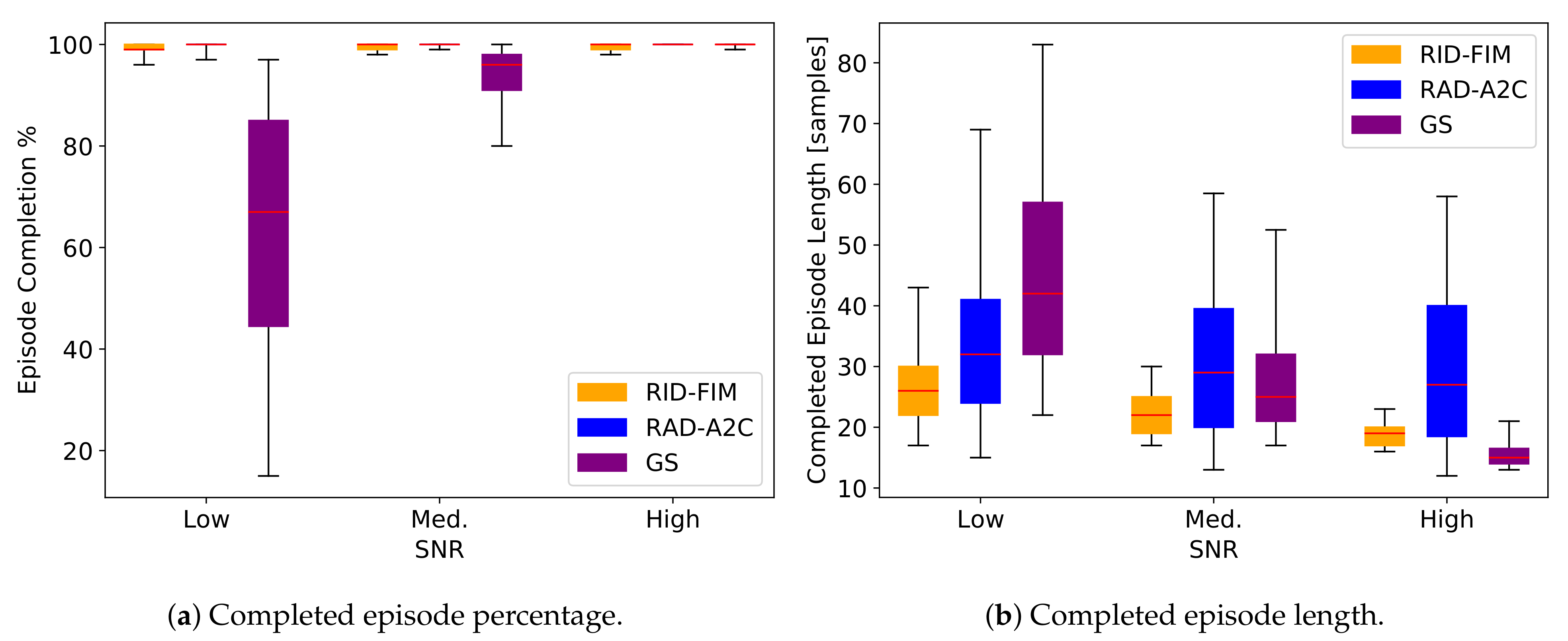
Box plots for the completed episode percentage and completed episode length for all methods in the convex environment are found in Figure 8a,b, respectively. The median is denoted in red, the boxes range from the first to the third quartile and the whiskers extend to the th and th percentiles. GS achieved the shortest episode completion length for all experiments at high SNR but performance decreased swiftly at the lower SNR levels. The RID-FIM had a consistent performance with tight boxes for both metrics at all SNR groups. The RAD-A2C was the only algorithm to maintain completion for all SNRs with the tradeoff being the longest median episode length for all but one of the SNRs.
3.3. Discussion
The results indicate close search performance between the RID-FIM and RAD-A2C algorithms in the convex environment. GS had the shortest episode completion length at high SNR but this required 7 more measurements per action selection. The RAD-A2C showed the best reliability in completing all of the episodes with a minimal spread in the distribution of results but had a greater spread in the completed episode length even at the highest SNR. The longer completed episode length of the RAD-A2C could be due to learned behavior that is advantageous in non-convex environments as the training environment always had obstructions present. The RID-FIM had a tighter and lower distribution of completed episode lengths across the SNRs.
Completion of episodes is the priority in practice as this will eliminate the threat of human harm from nuclear materials. Both algorithms get the job done effectively, however, the RID-FIM has a slightly greater chance of failing when SNR conditions are poor compared with the RAD-A2C. The RID-FIM utilized perfect knowledge of the background rate, which is a reasonable assumption in this particular source search context, however, its performance is likely to be degraded to some degree when it must also estimate an unknown background rate. The RAD-A2C did not receive the true episode background rate directly but did have prior exposure to the interval of background rates through training. Additionally, the RAD-A2C input standardization performs a moving average filter on the radiation measurement inputs (see Appendix A.2).
3.4. BPF Comparison
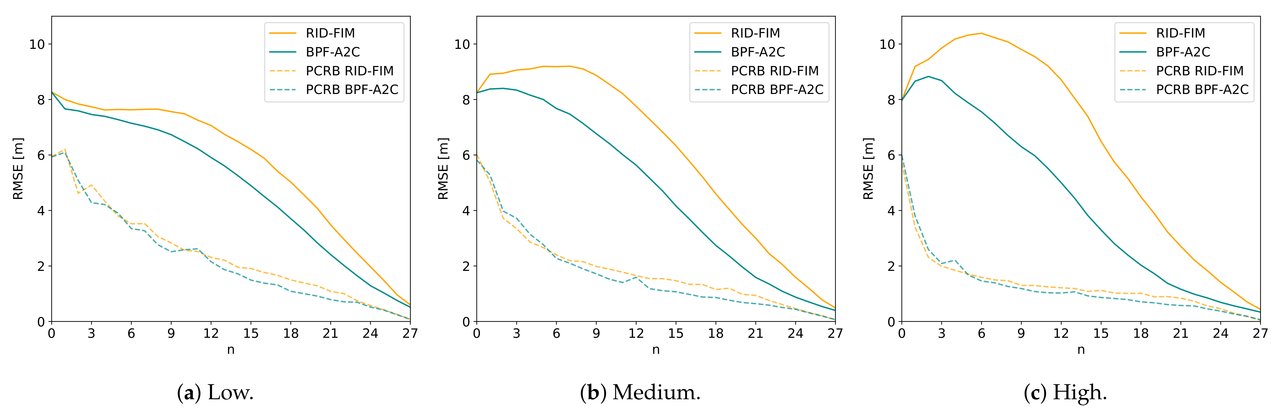
The RID-FIM and A2C controller are compared directly by replacing the PFGRU in the RAD-A2C with the BPF. This new system will be denoted as BPF-A2C in the following plots. Swapping in the BPF for the PFGRU facilitates in-depth analysis of the controllers through the lens of the BPF performance. The estimator performance depends entirely on the quality of action selection throughout an episode as this determines what information the estimates will be based on. Thus, we compare the RMSE for the Euclidean distance between the actual and predicted source location at each timestep for three different episode completion lengths across SNR. The BPF utilizes the current and previous observations (through the particle weights) to make a source location prediction. This comparison reveals the advantage of the A2C that uses both the BPF source location prediction and the current and previous observations (encoded in the hidden state) to inform action selection. In contrast, both the RID (Equation (A16)) and FIM (Equation (A13)) only utilize the source location prediction to inform action selection.
Figure 9, Figure 10 and Figure 11, show the RMSE and posterior Cramér-Rao lower bound (PCRB) for the RID-FIM and the BPF-A2C for three different completed episode lengths across SNRs. The PCRB serves as a proxy for the sub-optimality of the controllers because of the use of the same estimator (see Appendix B.5). Each plot is averaged over at least 200 different episodes and at least 700 total runs. An episode was only considered for this analysis if the completed episode length was the same for both algorithms in the set of the Monte Carlo runs for that episode ensuring that RMSEs and PCRBs were only averaged over the same set of episodes (same set of environment conditions). This gives a Bayesian Monte Carlo estimate on the estimator RMSE over the distribution of initial environment arrangements [31].
These specific completed episode lengths were chosen to highlight a variation in estimator performance. The RMSE for the RID-FIM is lower or equal to the BPF-A2C at a completed episode length of 17 across SNR. This changes for a completed episode length of 20 where the RID-FIM RMSE is only lower than the BPF-A2C at the lowest SNR. For the completed episode length of 28, the BPF-A2C now has a lower RMSE than the RID-FIM for all SNRs. In all of the plots, the PCRB for the BPF-A2C is slightly lower or equal to the PCRB for the RID-FIM. The PCRB decreases at a faster rate for the high SNR compared to the low SNR. Estimator RMSE consistently approaches the PCRB by the end of an episode. The RMSE initially increased for the high SNR in direct relation with the completed episode length in all the RMSE plots shown.
3.5. Discussion
The BPF serves as an interesting comparison point between the A2C and RID-FIM controllers. When the completed episode length was short (<16 samples), the RID-FIM location prediction RMSE was lower than the BPF-A2C and closer to the PCRB at all SNRs. This evidences the effectiveness of information-driven search schemes and the near-optimal performance of the RID-FIM when the BPF does not make spurious estimates. However, the occurrence of the intersection point of the RMSE curves highlights the disadvantage of the RID-FIM’s reliance on the estimator for action selection. If early state estimates are incorrect, this leads the RID-FIM to take more sub-optimal actions until the estimate is corrected. This is evidenced by the longer completed episode lengths () that have a greater initial increase in the RMSE as seen in Figure 10c and Figure 11c. Interestingly, the higher SNR contributes a sharper increase, likely due to the strong radiation measurements being interpreted by the BPF as evidence for the incorrect estimate.
In contrast, the A2C module of the BPF-A2C selects its actions from the location prediction and the measurement directly. Thus, when the SNR is high, the RMSE intersection point occurs at an earlier completed episode length (17 samples) because the A2C factors in measurement information at each timestep, rather than strictly following the possibly incorrect location prediction as the RID-FIM must do. This also explains why the BPF-A2C has lower RMSE at longer completed episode lengths as seen in Figure 11. The intersection point occurred at longer completed episode lengths for lower SNR because it takes the A2C longer to come across informative measurements that can correct the spurious BPF state estimates.
3.6. Non-Convex Environment
Detector Path Examples
Two detector paths for the RAD-A2C and the GS in two non-convex environments with three and seven obstructions are shown in Figure 12a,b, respectively.
The source prediction marker was omitted to reduce clutter. The GS takes many more samples to find a radiation gradient in the three obstruction environment but eventually finds the source. Gradient information is extremely sparse in the seven obstruction environment and thus the GS only moves randomly. The RAD-A2C can avoid the obstructions and find the source in both situations, even moving diagonally between two obstructions in Figure 12b. As in the convex environment, the majority of the RAD-A2C movements are in the cardinal directions.
3.7. Performance
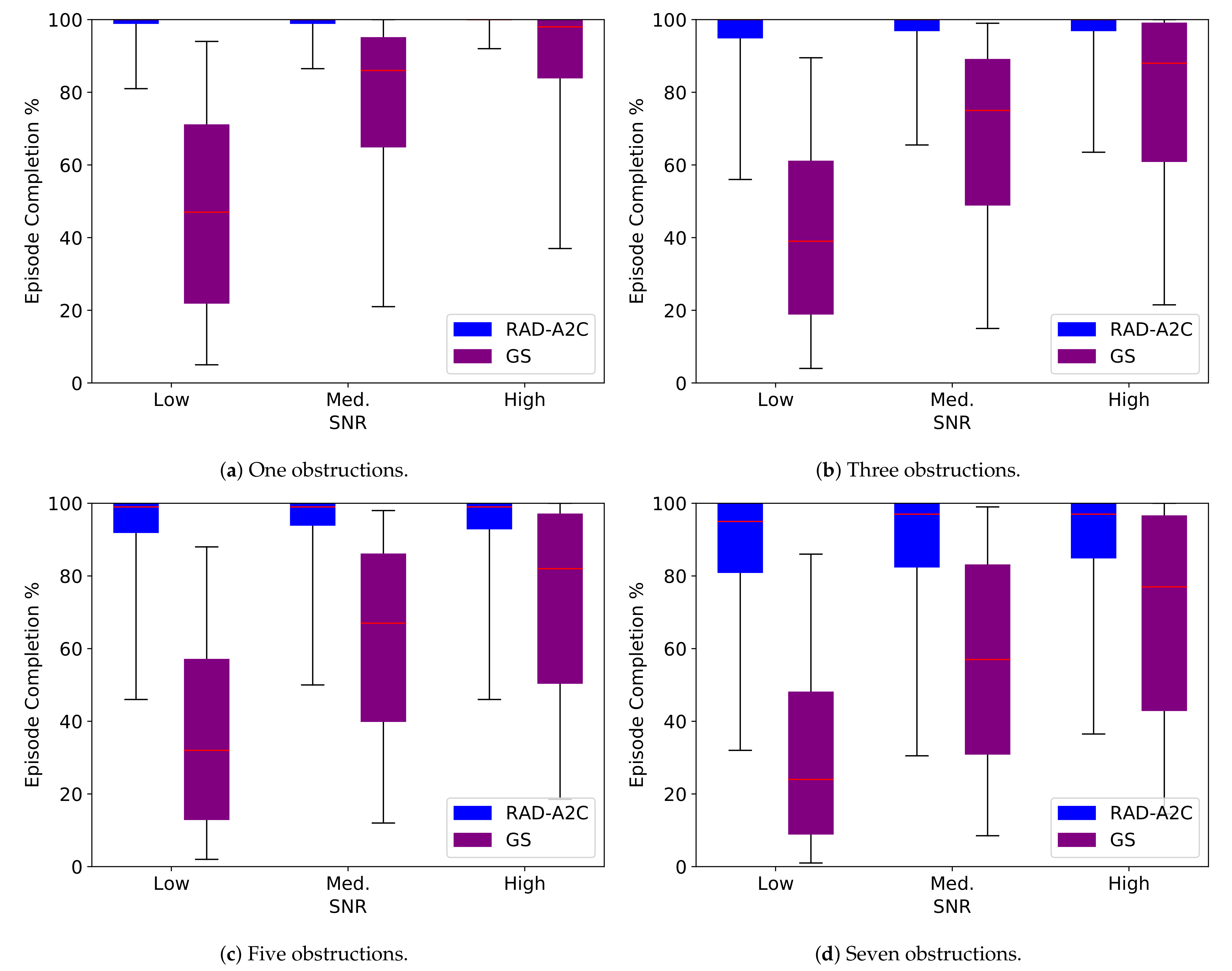
Box plots for the episode completion percentage and completed episode length against SNR for both methods in the non-convex environment are found in Figure 13 and Figure 14, respectively. Figure 13a and Figure 14a are results with one obstruction, Figure 13b and Figure 14b are results with three obstructions, Figure 13c and Figure 14c are results with five obstructions, and Figure 13d and Figure 14d are results with seven obstructions. The median is denoted in red, the boxes range from the first to the third quartile and the whiskers extend to the th and th percentiles.
Across obstruction number, the RAD-A2C maintains above episode completion even at low SNR. The distribution of the RAD-A2C episode completion gets larger as the number of obstructions increases. GS has >85% episode completion when there are less than 7 obstructions at high SNR but sees a sharp decrease in performance as the SNR level decreases. Even at high SNR, GS only completes of episodes when 7 obstructions are present. GS also has significant spread in the first and third quartile for most of the completed episode non-convex experiments. The RAD-A2C median for completed episode length increases by approximately 10 samples from a single obstruction to seven obstructions. The first and third quartiles for completed episode length also increase as the number of obstructions increase.
3.8. Non-Convex Environment
The results showcase the strong performance of the RAD-A2C in the non-convex environment. Surprisingly, the episode completion percentage did not decrease substantially in the seven obstruction configuration and the median completed episode length did not increase drastically. This demonstrates the algorithm’s ability to generalize as it was only trained on up to five obstructions per environment. The RAD-A2C is not simply a gradient search algorithm as the non-convex environment has many areas with no gradient information as evidenced by the ineffectiveness of the GS. Overall, these results support our hypothesis that the RAD-A2C is an effective search algorithm for both convex and non-convex environments.
4. Conclusions and Future Work
This paper investigated the efficacy of PPO and our proposed DRL architecture, the RAD-A2C, for a convex and non-convex radiation source search through comparison against the RID-FIM and GS across SNR. The GS had strong performance when the SNR was high but quickly lost efficacy with decreasing SNR. The RID-FIM typically required fewer measurements to complete episodes but had a slightly greater chance of not completing all of the episodes at lower SNRs. The RAD-A2C consistently completed all episodes albeit at the cost of taking more measurements. Guaranteed episode completion is arguably the most important criteria for radiation source search applications.
Estimator performance served as another lens to compare the controller performance directly. The same BPF was used for both controllers (RID-FIM, A2C) so that the RMSE and PCRB for the location prediction could be compared. We found that on average, the BPF RMSE was lower for the longer episode lengths when the A2C was the controller as it was able to factor in measurements to its action selection, as opposed to the RID-FIM which selected actions solely on the BPF location prediction. The RID-FIM’s action selection scheme is well-motivated but is susceptible to incorrect state estimates from the estimator.
In the non-convex environment, the RAD-A2C completed greater than of episodes over a range of obstructions and SNRs. There was very little gradient information available in the environments with more obstructions and thus the GS algorithm completed a much lower percentage of episodes. The RAD-A2C demonstrated generalizability as it was able to maintain a high completion percentage in a seven obstruction environment that it had never been trained on.
As mentioned in Section 2.3, the RAD-A2C formulation has the potential to be applied to other variations of the radiation source search. These include moving and/or shielded nuclear sources, spatially varying background rates, utilizing an attenuation model for different environment materials, locating an unknown number of multiple sources, and a larger, more complex urban environment such as the one used by Hite et al. [8]. A classification layer could also be added to the A2C module that is trained on detecting whether a source is present or not and how many sources are present. Noise could be added to the other dimensions of the observation vector such as the detector coordinates and/or the obstruction range measurements. In theory, the majority of these cases only require modification of the simulation environment, clever shaping of the reward signal, and hyperparameter sweeps to determine the model parameters.
Our proposed algorithm could be trained in a more realistic environment and gamma sensor simulation such as the one utilized for a single UAV source search by Baca et al. [32]. The authors developed a realistic gamma radiation simulation plugin for the Gazebo/ROS environment. Gazebo is a realistic open-source robotics simulator [33]. This plugin could then be easily interfaced with our DRL algorithm using the OpenAI_ROS Gym developed by Ezquerro et al. that seamlessly connects Gazebo and OpenAI Gym interfaces [34].
After training in a more realistic simulation environment, the trained network could then be evaluated in a real scene. For a real field application, a 7.6 cm diameter by 7.6 cm length cylindrical NaI detector is fairly common and could be used. NaI detectors were measured to have a peak resolution at 662 keV of (FHWM/centroid), sufficient to discriminate the full energy peak from most of the Compton scatter. As the low energy portion of the spectrum overlaps more with background radiation, without developing a background correction it is easier use the more easily identified peak for localization. With additional identification algorithms and higher resolution detectors, more complicated spectra could certainly be used.
Author Contributions
Conceptualization, P.P., C.T., A.H. and M.O.; methodology, P.P.; software, P.P.; validation, P.P.; formal analysis, P.P.; investigation, P.P.; resources, C.T. and M.O.; data curation, P.P.; writing—original draft preparation, P.P.; writing—review and editing, P.P., C.T., A.H. and M.O.; visualization, P.P.; supervision, C.T. and A.H.; project administration, C.T.; funding acquisition, C.T. and M. O. All authors have read and agreed to the published version of the manuscript.
Funding
This study was supported by the Defense Threat Reduction Agency under the grant HDTRA1-18-1-0009.
Acknowledgments
The authors would like to thank their colleague Merlin Carson for his support throughout this project. They would also like to thank Ren Cooper and Tenzing Joshi of Lawrence Berkeley National Laboratory along with Jason Hite from Oak Ridge National Laboratory for their correspondence and helpful suggestions.
Conflicts of Interest
The authors declare no conflict of interest.
Abbreviations
The following abbreviations are used in this manuscript:
| A2C | Advantage actor-critic |
| BPF | Bootstrap particle filter |
| BPF-A2C | Bootstrap particle filter and actor-critic |
| CRB | Cramér-Rao lower bound |
| DRL | Deep reinforcement learning |
| DL | Deep learning |
| FIM | Fisher information matrix |
| GRU | Gated recurrent unit |
| GS | Gradient search |
| LOS | Line-of-sight |
| NLOS | No line-of-sight |
| ML | Machine learning |
| PCRB | Posterior Cramér-Rao lower bound |
| PFGRU | Particle filter gated recurrent unit |
| PPO | Proximal policy optimization |
| RAD-A2C | Our proposed actor-critic architecture |
| RNN | Recurrent neural network |
| RID | Rényi information divergence |
| RID-FIM | Hybrid information-driven controller that uses RID and FIM |
| RL | Reinforcement learning |
| SNR | Signal-to-noise ratio |
Appendix A. RAD-A2C
Appendix A.1. Particle Filter Gated Recurrent Unit (PFGRU)
The PFGRU is an embedding of the BPF into a GRU architecture proposed by Ma et al [29]. As in the BPF, there are a set of particles and weights used for filtering and prediction of the posterior state distribution. In the case of the PFGRU, the particles are represented by the set of hidden or latent state vectors, . The latent states are propagated and the weights updated at each timestep by a learned transition and measurement function denoted as,
where is a learned noise term akin to the process noise in the BPF and denotes the source location prediction. The weight update also relies on a learned likelihood function,
where is a normalization factor.
The PFGRU utilizes a soft resampling scheme to combat particle degeneracy while maintaining model differentiability. This is achieved by sampling particle indices from a multinomial distribution with probabilities determined by a convex combination of a uniform distribution and the particle weight distribution. The new weights are then determined by,
where is the mixture coefficient parameter. The new latent states, , are resampled from the previous latent states using a multinomial distribution over particle indices with probability equal to the particle weights. The loss function consists of two components to capture the important facets of state space tracking. The first component is the mean squared loss between the mean particle source location prediction and the and the true source location. The second component is the evidence lower bound (ELBO) loss that measures the difference in distribution of the particle distribution relative to the observation likelihood, for more details see [29]. The total loss is expressed as,
where is a weighting parameter determined by the user. Figure A1 shows the PFGRU architecture.
Figure A1.
PFGRU Architecture. The hidden state and weights are elements of a set of size . Each box represents a weight matrix and activation function and the circles represent mathematical operations. The conjoining lines represent concatenation of the quantity and diverging lines represent the copying. The crux of the reset () and update () gates are to modify the candidate hidden state () which then becomes the output hidden state (). The hidden state and weights are resampled using a soft-resampling scheme at each timestep to preserve differentiability. Recreated from [29].

Appendix A.2. Training
The estimate of the gradient iterate Equation (11) is improved by increasing the number of histories being averaged over. Schulman et al. improved training scalability by instantiating copies of the DRL agent and environment on different CPU cores to parallelize episode collection [25]. Each DRL agent computes its parameter gradients after all episodes for an epoch have been collected. The gradients are then averaged across all the cores and a weight update is performed per core. An important distinction in the implementation used here is the environment variation across the CPU cores. All of the sampled quantities were different per core and fixed per epoch resulting in a more generalized policy. This is because the averaged gradient step will be in the direction that improves performance across a diverse set of environments. Tobin et al. proposed a similar idea called domain randomization that aimed to bridge the gap between DRL simulators and reality by introducing extra variability into the simulator [17]. Table A1 shows the hyperparameters that resulted in the strongest performance for the DRL agent from the parameter sweep. The total training time for a single DRL agent running on 10 cores took approximately 26 hrs. The PFGRU added considerable training overhead but resulted in the best performance. Future work should experiment with different localization modules or using a pretrained PFGRU. A graphics processing unit did not provide a speedup in training due to the variation in episode length per epoch. This required that the episodes be fed to the network serially.

Table A1.
Hyperparameter values with the strongest performance for the DRL agent from our parameter sweep. The parameter c is the loss weighting coefficient for the value function loss. The parameters and are used in the generalized advantage estimator [24]. The parameter is the maximum value for the approximate Kullback-Leibler divergence before weight updates are terminated for the epoch.
| Parameter | Value |
|---|---|
| Epochs | 3000 |
| Episodes per epoch | 4 |
| Num. cores | 10 |
| Tot. weights & biases | 7443 |
| GRU hidden size | 24 |
| PFGRU hidden size | 24 |
| PFGRU particles | 40 |
| Learning Rate A2C | |
| Learning Rate PFGRU | |
| Optimizer | Adam |
| c | 0.01 |
| (,,) |
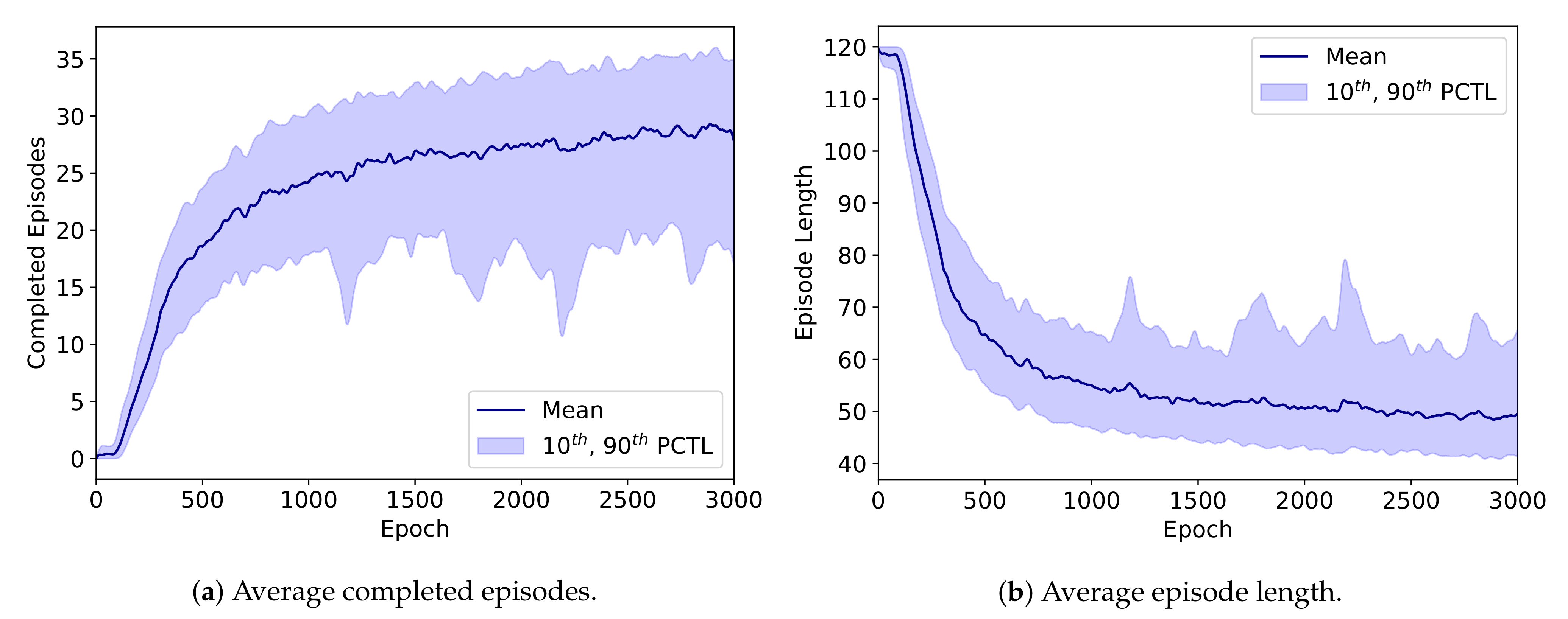
The RAD-A2C was trained eight separate times with eight different random seeds to assess model stability. In seven of the eight models, the RAD-A2C achieved training curve performance that was consistent with the model we used for the assessment in this paper. This is evidenced by the training curves in Figure A2 that show the average number of completed episodes and the average episode length over the 10 parallelized environments per epoch. The dark blue line represents the smoothed mean and the shaded region represents the smoothed 10th and 90th percentiles over the eight random seeds. The maximum possible number of completed episodes per epoch was 40. The one model that did not converge as well as the others showed oscillations in the performance curves indicating that a parameter update resulted in an adverse policy change. Training for more than 3000 epochs did not significantly improve performance.
Figure A2.
Performance curves during the training process for the RAD-A2C over eight random seeds. (a) shows the number of completed episodes and (b) shows the episode length averaged over the 10 parallelized environments per epoch. The dark blue line represents the smoothed mean and the shaded region represents the smoothed 10th and 90th percentiles over the eight random seeds. Episode length decreases and number of completed episodes increases as the model converges to a useful policy. Training for more than 3000 epochs did not significantly improve performance.

Appendix A.3. Standardization
A common technique in DL is to standardize the input data to increase training stability and speed. This is done by subtracting the mean and dividing by the standard deviation per feature across a batch of input data. The DRL context does not have easy access to the full data statistics since it is collected and processed online. We used a technique proposed by Welford for estimating a running sample mean and variance as follows [35],
where , . The statistics were updated after each new observation and then standardization was performed. The quantities were reset to 0 after an episode was completed.
Appendix B. Information-Driven Controller
Information-driven search is an information-theoretic framework for sequential action selection. This framework endows the controller with the ability to update its path plan as new observations become available as opposed to relying only on whether the target has been detected or not [36]. Information is integrated across time by tracking the posterior probability density of states of interest. This can quickly become computationally prohibitive and so heuristic methods such as the bootstrap particle filter (BPF) are employed.
Appendix B.1. Bootstrap Particle Filter (BPF)
The BPF is typically used to track a dynamic process over time. It has been proven that an optimal estimate of the state can be recovered from the posterior state distribution, however, it is often computationally intractable to track when the state dimension is high [37]. Thus, methods such as the BPF attempt to approximate the posterior state through a set of samples, , often referred to as particles and weights, respectively. This leads to the approximation,
where is the marginal posterior over the states of interest, is the particle weight, is the particle, is the Dirac Delta function, and is the number of particles. At each timestep, the particles are propagated through the process model and a measurement prediction is generated with the measurement model. The particle weights are calculated recursively as,
where is the measurement likelihood, is the transition density, and is an importance density [37]. Particles are drawn from a user-specified importance density . In our implementation, the importance density is set equal to the prior distribution to reduce the weight update step to the measurement likelihood and the previous weight:
If a particle has a low probability for a given measurement, this effectively removes the particle’s contribution to the estimated posterior which can adversely affect state estimation over the trajectory and is known as the degeneracy problem. Particle degeneracy can be tracked by the following metric to characterize the number of effective particles at a given time step,
Particle degeneracy can be alleviated by resampling the particles and reinitializing the weights when the number of effective particles becomes too low. In our context, the nuclear source intensity and coordinates are fixed throughout an episode. We adapt the BPF for parameter estimation with a random walk process model that has low variance Gaussian noise. The initial particles were sampled uniformly from fixed intervals as specified in Table A2. Equations (2) and (3) are the measurement model and likelihood, respectively. The background rate, , was considered constant and known.
Sequential importance resampling is a technique to combat particle degeneracy and occurs when the number of effective particles drops below a given threshold. We selected the Srinivasan sampling process (SSP) resampling proposed by Gerber et al. because of asymptotic convergence of the error variance [38]. Additionally, SSP resampling requires only operations. See [38,39] for more details.
Appendix B.2. Fisher Information Matrix (FIM)
The FIM is a measure of the information content of a measurement relative to the measurement model. It was first used in optimal observer motion for bearings-only tracking by Hammel et al. [40]. In their implementation, the controller selects the action at each timestep that maximizes the determinant of the FIM (system observability), which is equivalent to minimizing the area of the uncertainty ellipsoids around the state estimates. This arises from the connection between the FIM and the Cramér-Rao lower bound (CRB).
The CRB provides a lower bound on the error covariance of an unbiased estimator and is the inverse of the FIM [41]. The FIM is the Hessian of the log-likelihood and is denoted as follows,
where T denotes the transpose. Morelande et al. derived the closed form FIM for the radiation source localization problem as [7],
where is defined in Equation (2). This results in the following gradient for each parameter,
Ristic et al. used the BPF particles at each time step to calculate the FIM as follows,
due to better performance when the posterior is multi-modal [11]. They applied this formulation to action selection in the radiation source search in the following manner,
where L is the number of lookahead steps, tr() is the matrix trace, and is the control vector that determines the detector’s next position.
Helferty et al. proposed to use the trace of the CRB as it is a sum of squares of the axes of the uncertainty ellipsoid [42]. This is also known as A-optimality in the optimal experimental design literature [43]. Ristic et al. maximized the trace of the FIM that corresponds to maximizing the information, however, it is beyond the scope of this paper to show the relation between these two criteria. This control strategy will result in the optimal trajectory for minimizing the uncertainty of the estimated quantities given perfect source information (i.e., low or no measurement error). The source information in the nuclear source search context is not perfect due to the stochastic nature of nuclear decay and background radiation. Additionally, the FIM is not well defined for initial search conditions where the background radiation dominates the signal from the source, i.e., when the source-detector distance is large and/or the background rate is high.
Appendix B.3. Rényi Information Divergence (RID)
Ristic et al. proposed another information-driven search strategy to address the shortcomings of the FIM-based approach. This approach is based upon the RID, also known as -divergence, a general information metric that quantifies the difference between two probability distributions. In Bayesian estimation, maximizing this difference corresponds to reducing the uncertainty around the state estimates. The use of RID was first proposed in the sensor management context by Kreucher et al. [44]. The RID is defined as,
where specifies the order. In the limit as approaches one, the RID approaches the Kullback-Leibler Divergence [44].
Ristic et al. adapted the RID for action selection in the nuclear source search context with a BPF [12]. The general flow of the algorithm is to apply an action from the set of actions to get the next potential detector position, calculate the expected posterior density for that action over a measurement interval, and then select the action that resulted in the greatest RID. The particle approximation of the RID is shown in the following equation,
where denotes the potential detector position after taking action , is a measurement interval, and . The density is approximated after filtering the latest measurement and particle resampling as,
and results from the particle approximation of the marginal distribution of a measurement. Like the FIM, the RID can also be computed for L-step planning.
Appendix B.4. Hybrid RID-FIM Controller
We propose a hybrid controller that utilizes either the RID or FIM as metrics for action selection. This was motivated in part by the empirical observation that the RID controller would often get stuck oscillating between two positions that were just above our termination criteria for source-detector distance resulting in incomplete episodes. The FIM is a poor control metric when there is little information available as is often the case at the start of a search. The RID is more computationally expensive than the FIM but provides a principled control method even in low information contexts. Thus, the RID was used for control at the beginning of each episode until the RID reached a sufficient threshold, then the metric was switched over to the FIM for the remainder as shown in Algorithm A1.
| Algorithm A1 RID-FIM Controller. |
| Input:, set RID FLAG to 1, switch threshold , effective particles threshold , measurement interval Receive init. measurement, , perform prediction and filtering of particles while episode not terminated do if RID FLAG then Calculate RID according to Equation (A16) over if RID > then Set RID FLAG to 0 end if else Calculate FIM according to Equation (A13) end if Select action that maximizes information metric Receive , perform prediction and filtering of particles if then Resample and reweight particles end if end while |
We decided on myopic (one-step lookahead) planning due to the exponential increase in computational cost inherent to both metric calculations. Additionally, many source search scenarios will have high uncertainty in the state estimates for many timesteps so planning far in advance is not advantageous. Myopic search is often sub-optimal but is a fair tradeoff when the problem dynamics are stable [44]. The parameter values for the RID-FIM, as well as the BPF, are detailed in Table A2. All parameters were selected by a parameter sweep over a set of 100 randomly sampled environments where the selection criteria was shortest average episode length and most episodes completed.
Table A2.
Parameter values for the BPF and RID-FIM. The source intensity was
| Parameter | Value |
|---|---|
| 6000 | |
| 6000 | |
| Process noise XY | m |
| Process noise | gps |
| Prior XY | m |
| Prior | gps |
| Resampling threshold, | |
| Lookahead, L | 1 |
| Order, | |
| Switch threshold, | |
| Meas. interval | cps |
Appendix B.5. Posterior Cramér-Rao Lower Bound (PCRB)
The BPF is a biased estimator as it only uses a finite number of particles. The PCRB provides a lower bound on the root-mean-square error (RMSE) performance for a biased estimator. Tichavsky proposed the PCRB for discrete-time nonlinear filtering [45], however, we follow a similar formulation found in Bergman’s dissertation [31]. The PCRB is determined recursively in the following manner,
where the terms and are all the same inverse process noise covariance matrix, denoted as . This arises from the fact that our process model is a random walk with Gaussian noise for each state. The term is the FIM defined in Equation (A10). The prior, , is a result of the uniform distribution of the particles where is a diagonal matrix of the uniform probabilities for each parameter. More details of the derivation of the PCRB and prior can be found in Bergman’s dissertation in Theorem and Section , respectively [31].
We average the RMSE and PCRB over the Monte Carlo evaluations resulting in the following formulation,
where K is the total number of episodes and ≳ denotes that the inequality only holds approximately for finite K [31]. The PCRB provides an indicator of the suboptimality of an estimator and so we use it to directly compare the performance of the A2C with the RID-FIM. This is accomplished by evaluating the A2C with the exact same BPF estimator used with the RID-FIM for the source location state estimates. Not only can the estimator RMSE be compared against the PCRB, but the PCRBs resulting from both controllers can be compared as well. This will serve as a proxy for the quality of the control path generated by each controller.
Appendix C. Gradient Search
We use the simple GS algorithm implemented by Liu et al. [16]. GS relies on sampling the gradient of the radiation field for each search direction at each timestep. This is not an efficient algorithm as the detector must make D moves per action selection but serves as a useful baseline for performance comparison. The action selection is made stochastic by sampling from a multinomial distribution, denoted multi(n,p), over actions with probabilities proportional to the softmax of the gradients to avoid the trapping of local optima. GS is summarized by the following equation,
where u is the detector position after action i, is the softmax function, and q is a temperature parameter. The temperature parameter was set at and was determined via a parameter sweep over a set of 100 randomly sampled environments where the selection criteria was shortest average episode length and most episodes completed.
References
- Sieminski, A. International energy outlook. Energy Inf. Adm. (EIA) 2014, 18, 2. [Google Scholar]
- The United Nations Scientific Committee on the Effects of Atomic Radiation. Sources and Effects of Ionizing Radiation; United Nations Publications: New York City, NY, USA, 2008; Volume 1. [Google Scholar]
- Nagatani, K.; Kiribayashi, S.; Okada, Y.; Otake, K.; Yoshida, K.; Tadokoro, S.; Nishimura, T.; Yoshida, T.; Koyanagi, E.; Fukushima, M.; et al. Emergency response to the nuclear accident at the Fukushima Daiichi Nuclear Power Plants using mobile rescue robots. J. Field Robot. 2013, 30, 44–63. [Google Scholar] [CrossRef]
- Knoll, G.F. Radiation Detection and Measurement; John Wiley & Sons: Hoboken, NJ, USA, 2010. [Google Scholar]
- Curto, C.; Gross, E.; Jeffries, J.; Morrison, K.; Omar, M.; Rosen, Z.; Shiu, A.; Youngs, N. What makes a neural code convex? SIAM J. Appl. Algebra Geom. 2017, 1, 222–238. [Google Scholar] [CrossRef] [Green Version]
- Silver, D.; Schrittwieser, J.; Simonyan, K.; Antonoglou, I.; Huang, A.; Guez, A.; Hubert, T.; Baker, L.; Lai, M.; Bolton, A.; et al. Mastering the game of Go without human knowledge. Nature 2017, 550, 354–359. [Google Scholar] [CrossRef] [PubMed]
- Morelande, M.; Ristic, B.; Gunatilaka, A. Detection and parameter estimation of multiple radioactive sources. In Proceedings of the 2007 10th International Conference on Information Fusion, Quebec, QC, Canada, 9–12 July 2007; pp. 1–7. [Google Scholar]
- Hite, J.; Mattingly, J. Bayesian Metropolis methods for source localization in an urban environment. Radiat. Phys. Chem. 2019, 155, 271–274. [Google Scholar] [CrossRef]
- Hellfeld, D.; Joshi, T.H.; Bandstra, M.S.; Cooper, R.J.; Quiter, B.J.; Vetter, K. Gamma-ray point-source localization and sparse image reconstruction using Poisson likelihood. IEEE Trans. Nucl. Sci. 2019, 66, 2088–2099. [Google Scholar] [CrossRef]
- Cortez, R.; Papageorgiou, X.; Tanner, H.; Klimenko, A.; Borozdin, K.; Priedhorsk, W. Experimental implementation of robotic sequential nuclear search. In Proceedings of the 2007 Mediterranean Conference on Control & Automation, Athens, Greece, 27–29 June 2007; pp. 1–6. [Google Scholar]
- Ristic, B.; Gunatilaka, A. Information driven localisation of a radiological point source. Inf. Fusion 2008, 9, 317–326. [Google Scholar] [CrossRef]
- Ristic, B.; Morelande, M.; Gunatilaka, A. Information driven search for point sources of gamma radiation. Signal Process. 2010, 90, 1225–1239. [Google Scholar] [CrossRef]
- Ristic, B.; Morelande, M.; Gunatilaka, A. A controlled search for radioactive point sources. In Proceedings of the 2008 11th International Conference on Information Fusion, Cologne, Germany, 30 June–3 July 2008; pp. 1–5. [Google Scholar]
- Anderson, R.B.; Pryor, M.; Abeyta, A.; Landsberger, S. Mobile Robotic Radiation Surveying With Recursive Bayesian Estimation and Attenuation Modeling. IEEE Trans. Autom. Sci. Eng. 2020, 1–15. [Google Scholar] [CrossRef]
- Landgren, P.C. Distributed Multi-Agent Multi-Armed Bandits. Ph.D. Thesis, Princeton University, Princeton, NJ, USA, 2019. [Google Scholar]
- Liu, Z.; Abbaszadeh, S. Double Q-learning for radiation source detection. Sensors 2019, 19, 960. [Google Scholar] [CrossRef] [Green Version]
- Tobin, J.; Fong, R.; Ray, A.; Schneider, J.; Zaremba, W.; Abbeel, P. Domain randomization for transferring deep neural networks from simulation to the real world. In Proceedings of the 2017 IEEE/RSJ International Conference on Intelligent Robots and Systems (IROS), Vancouver, BC, Canada, 24–28 September 2017; pp. 23–30. [Google Scholar]
- Wierstra, D.; Förster, A.; Peters, J.; Schmidhuber, J. Recurrent policy gradients. Log. J. IGPL 2010, 18, 620–634. [Google Scholar] [CrossRef]
- Beigzadeh, A.M.; Vaziri, M.R.R.; Soltani, Z.; Afarideh, H. Design and improvement of a simple and easy-to-use gamma-ray densitometer for application in wood industry. Measurement 2019, 138, 157–161. [Google Scholar] [CrossRef]
- Brockman, G.; Cheung, V.; Pettersson, L.; Schneider, J.; Schulman, J.; Tang, J.; Zaremba, W. OpenAI gym. arXiv 2016, arXiv:1606.01540. [Google Scholar]
- Henderson, P.; Islam, R.; Bachman, P.; Pineau, J.; Precup, D.; Meger, D. Deep reinforcement learning that matters. In Proceedings of the AAAI Conference on Artificial Intelligence, New Orleans, LA, USA, 2–7 February 2018; Volume 32. [Google Scholar]
- Sutton, R.S.; Barto, A.G. Reinforcement Learning: An Introduction; MIT Press: Cambridge, MA, USA, 2018. [Google Scholar]
- Tesauro, G. Temporal difference learning and TD-Gammon. Commun. ACM 1995, 38, 58–68. [Google Scholar] [CrossRef]
- Schulman, J.; Moritz, P.; Levine, S.; Jordan, M.; Abbeel, P. High-dimensional continuous control using generalized advantage estimation. arXiv 2015, arXiv:1506.02438. [Google Scholar]
- Schulman, J.; Wolski, F.; Dhariwal, P.; Radford, A.; Klimov, O. Proximal policy optimization algorithms. arXiv 2017, arXiv:1707.06347. [Google Scholar]
- Andrychowicz, M.; Raichuk, A.; Stańczyk, P.; Orsini, M.; Girgin, S.; Marinier, R.; Hussenot, L.; Geist, M.; Pietquin, O.; Michalski, M.; et al. What matters in on-policy reinforcement learning? A large-scale empirical study. arXiv 2020, arXiv:2006.05990. [Google Scholar]
- Cho, K.; Van Merriënboer, B.; Bahdanau, D.; Bengio, Y. On the properties of neural machine translation: Encoder-decoder approaches. arXiv 2014, arXiv:1409.1259. [Google Scholar]
- Olah, C. Understanding LSTM Networks. 2015. Available online: http://colah.github.io/posts/2015-08-Understanding-LSTMs/ (accessed on 20 April 2021).
- Ma, X.; Karkus, P.; Hsu, D.; Lee, W.S. Particle filter recurrent neural networks. In Proceedings of the AAAI Conference on Artificial Intelligence, New York, NY, USA, 7–12 February 2020; Volume 34, pp. 5101–5108. [Google Scholar]
- Paszke, A.; Gross, S.; Massa, F.; Lerer, A.; Bradbury, J.; Chanan, G.; Killeen, T.; Lin, Z.; Gimelshein, N.; Antiga, L.; et al. PyTorch: An Imperative Style, High-Performance Deep Learning Library. Adv. Neural Inf. Process. Syst. 2019, 32, 8026–8037. [Google Scholar]
- Bergman, N. Recursive Bayesian Estimation: Navigation and Tracking Applications. Ph.D. Thesis, Linköping University, Linköping, Sweden, 1999. [Google Scholar]
- Baca, T.; Stibinger, P.; Doubravova, D.; Turecek, D.; Solc, J.; Rusnak, J.; Saska, M.; Jakubek, J. Gamma Radiation Source Localization for Micro Aerial Vehicles with a Miniature Single-Detector Compton Event Camera. arXiv 2020, arXiv:2011.03356. [Google Scholar]
- Koenig, N.; Howard, A. Design and Use Paradigms for Gazebo, An Open-Source Multi-Robot Simulator. In Proceedings of the IEEE/RSJ International Conference on Intelligent Robots and Systems, Sendai, Japan, 28 September–2 October 2004; pp. 2149–2154. [Google Scholar]
- Téllez, R.; Ezquerro, A.; Rodríguez, M.Á. ROS Manipulation in 5 Days: Entirely Practical Robot Operating System Training; Independently Published: Barcelona, Spain, 2017. [Google Scholar]
- Welford, B. Note on a method for calculating corrected sums of squares and products. Technometrics 1962, 4, 419–420. [Google Scholar] [CrossRef]
- Stone, L.D. OR Forum—What’s Happened in Search Theory Since the 1975 Lanchester Prize? Oper. Res. 1989, 37, 501–506. [Google Scholar] [CrossRef] [Green Version]
- Arulampalam, M.S.; Maskell, S.; Gordon, N.; Clapp, T. A tutorial on particle filters for online nonlinear/non-Gaussian Bayesian tracking. IEEE Trans. Signal Process. 2002, 50, 174–188. [Google Scholar] [CrossRef] [Green Version]
- Gerber, M.; Chopin, N.; Whiteley, N. Negative association, ordering and convergence of resampling methods. Ann. Stat. 2019, 47, 2236–2260. [Google Scholar] [CrossRef] [Green Version]
- Srinivasan, A. Distributions on level-sets with applications to approximation algorithms. In Proceedings of the 42nd IEEE Symposium on Foundations of Computer Science, Newport Beach, CA, USA, 8–11 October 2001; pp. 588–597. [Google Scholar]
- Hammel, S.; Liu, P.; Hilliard, E.; Gong, K. Optimal observer motion for localization with bearing measurements. Comput. Math. Appl. 1989, 18, 171–180. [Google Scholar] [CrossRef] [Green Version]
- Van Trees, H.L. Detection, Estimation, and Modulation Theory, Part I: Detection, Estimation, and Linear Modulation Theory; John Wiley & Sons: Hoboken, NJ, USA, 2004. [Google Scholar]
- Helferty, J.P.; Mudgett, D.R. Optimal observer trajectories for bearings only tracking by minimizing the trace of the Cramér-Rao lower bound. In Proceedings of the 32nd IEEE Conference on Decision and Control, San Antonio, TX, USA, 15–17 December 1993; pp. 936–939. [Google Scholar]
- Pronzato, L. Optimal experimental design and some related control problems. Automatica 2008, 44, 303–325. [Google Scholar] [CrossRef] [Green Version]
- Kreucher, C.; Kastella, K.; Hero Iii, A.O. Sensor management using an active sensing approach. Signal Process. 2005, 85, 607–624. [Google Scholar] [CrossRef]
- Tichavsky, P.; Muravchik, C.H.; Nehorai, A. Posterior Cramér-Rao bounds for discrete-time nonlinear filtering. IEEE Trans. Signal Process. 1998, 46, 1386–1396. [Google Scholar] [CrossRef] [Green Version]
Figure 1.
An autonomous mobile robot operating in a non-convex environment. The unshielded gamma source emits gamma radiation isotropically. Obstructions (gray cubes) attenuate the gamma radiation signal and block the robot’s path.
Figure 1.
An autonomous mobile robot operating in a non-convex environment. The unshielded gamma source emits gamma radiation isotropically. Obstructions (gray cubes) attenuate the gamma radiation signal and block the robot’s path.

Figure 2.
At every timestep , the agent receives an observation and reward . The observation consists of the fully observable state components and the state measurement, , that is conditioned on the state . The observation only gives partial information about the state. The state transition and the reward depend on taking action in state .

Figure 3.
A sample of the starting conditions for (a) convex and (b) non-convex environment. In both environment types, the red star is the source position, the black triangle is the detector position, and the magenta circle is the agent’s prediction of source position. In the non-convex environment, the gray rectangles are obstructions that block line of sight between the source and detector.

Figure 4.
Key data streams used by the DRL agent in training and inference. (a) shows the detector position at each timestep as it moves closer to the source. (b) shows the radiation counts measurements at each timestep corresponding with the detector position. (c) shows the cumulative reward signal that the DRL agent uses during training. The reward signal is only used for weight updates after all episodes in an epoch have been completed.

Figure 5.
(a) shows the input flow for an RNN where each is fed to the network sequentially. The learned weight matrices are the same across all sequence steps so the only changes are the input, output and hidden state. The represents the hidden state which is passed between sequence steps and is combined with the input to carry information across time. The output, , is mapped from the hidden state. (b) shows the GRU architecture, a variation on the in (a). Each box represents a weight matrix and activation function and the circles represent mathematical operations. The conjoining lines represent concatenation of the quantity and diverging lines represent the copying. The crux of the reset () and update () gates are to modify the candidate hidden state () which then becomes the output hidden state (). Recreated from [28].

Figure 6.
RAD-A2C source search architecture. The PFGRU provides a location prediction, denoted (), at each timestep, which is concatenated with the observation and fed into the A2C. The GRU module encodes the observations over time in its hidden state and the Actor layer selects an action from this hidden state. The Critic layer predicts the expected cumulative reward from the hidden state and is only needed during training. The dotted lines indicate the gradient flow during backpropagation.

Figure 7.
Three detector paths for the RAD-A2C, the RID-FIM, and the GS in high and low SNR configurations of the convex environment overlayed on a single plot. (a) shows a low SNR configuration and (b) shows a high SNR configuration. The green square denotes the detector starting position and the red star represents the radiation source.Triangles denote the detector position and point in the direction of the detector movement. A star-like marker results from the detector traveling to a position multiple times. In both cases, the stochastic nature of gamma radiation measurement results in the control algorithms taking sub-optimal actions before the source could be located.

Figure 8.
Box plots for the completed episode percentage and completed episode length against SNR in the convex environment. The median is denoted in red, the boxes range from the first to the third quartile and the whiskers extend to the th and th percentiles. Figure 8b shows the RID-FIM consistently found the source in a short amount of time even as SNR decreased. Figure 8a shows the RAD-A2C was the only method that completed of the episodes. GS performance sharply declined for lower SNRs.

Figure 9.
Comparison of the Monte Carlo RMSE for BPF estimation of the source location at each timestep for a completed episode length of 17. Each plot contains the BPF PCRB and RMSE for the RID-FIM and A2C controllers averaged over at least 200 different episodes. (a) is at low SNR, (b) is at medium SNR, and (c) is at high SNR. The RID-FIM has a lower RMSE than the BPF-A2C for the low and medium SNR but the RID-FIM’s action selection was solely dependent on potentially spurious BPF state estimates, which caused the BPF-A2C to match the RID-FIM performance at the high SNR.

Figure 10.
Comparison of the Monte Carlo RMSE for BPF estimation of the source location at each timestep for a completed episode length of 20. Each plot contains the BPF PCRB and RMSE for the RID-FIM and A2C controllers averaged over at least 400 different episodes. (a) is at low SNR, (b) is at medium SNR, and (c) is at high SNR. The RID-FIM has a lower RMSE than the BPF-A2C for the low SNR but the RID-FIM’s action selection was solely dependent on potentially spurious BPF state estimates, which caused the BPF-A2C to outperform the RID-FIM at medium and high.

Figure 11.
Comparison of the Monte Carlo RMSE for BPF estimation of the source location at each timestep for a completed episode length of 28. Each plot contains the BPF PCRB and RMSE for the RID-FIM and A2C controllers averaged over at least 650 different episodes. (a) is at low SNR, (b) is at medium SNR, and (c) is at high SNR. The BPF-A2C has a lower RMSE than then RID-FIM when the completed episode length was longer due to the RID-FIM’s action selection dependence on potentially spurious BPF state estimates.

Figure 12.
Two detector paths for the RAD-A2C and the GS overlayed on a single plot for the non-convex environment. (a) shows the three obstruction environment and (b) shows the seven obstruction environment. The green square denotes the detector starting position, the gray rectangles represent obstructions that block radiation propagation, and the red star is the radiation source. Triangles denote the detector position and point in the direction of the detector movement. A star-like marker results from the detector traveling to a position multiple times. Both algorithms must explore the area as they search for radiation signal above the noise floor.

Figure 13.
Box plots for the completed episode percentage against SNR in the non-convex environment, where each plot corresponds to a different number of obstructions in the environment. The median is denoted in red, the boxes range from the first to the third quartile and the whiskers extend to the th and th percentiles. (a) was for a single obstruction, (b) was for three obstructions, (c) was for five obstructions, and (d) was for seven obstructions. GS episode completion deteriorates with increasing number of obstructions while the RAD-A2C maintains greater than median episode completion.

Figure 14.
Box plots for the completed episode length against SNR in the non-convex environment, where each plot corresponds to a different number of obstructions in the environment. The median is denoted in red, the boxes range from the first to the third quartile and the whiskers extend to the th and th percentiles. (a) was for a single obstruction, (b) was for three obstructions, (c) was for five obstructions, and (d) was for seven obstructions. The RAD-A2C maintains a low completed episode length across the varying number of obstructions and SNR while GS performance deteriorates.

Table 1.
Radiation source simulation for convex and non-convex environment parameters. The brackets indicate an interval that was uniformly sampled on a per epoch basis. Src. and det. are abbreviations for source and detector, respectively.
Table 1.
Radiation source simulation for convex and non-convex environment parameters. The brackets indicate an interval that was uniformly sampled on a per epoch basis. Src. and det. are abbreviations for source and detector, respectively.
| Parameter | Value |
|---|---|
| Area Dimensions | |
| Src., det. initial positions | [0, 20] m |
| Src. rate | gps |
| Background rate | [10, 50] cps |
| State space | 11 |
| Action space | 8 |
| Max. search time | 120 samples |
| Velocity | 1 m/sample |
| Termination dist. | 1.1 m |
| Min. src.-det. initial dist. | 10 m |
| Number of obstructions | [1, 5] |
| Obstruction dim. | [2, 5] m |
Publisher’s Note: MDPI stays neutral with regard to jurisdictional claims in published maps and institutional affiliations. |
© 2021 by the authors. Licensee MDPI, Basel, Switzerland. This article is an open access article distributed under the terms and conditions of the Creative Commons Attribution (CC BY) license (https://creativecommons.org/licenses/by/4.0/).
Share and Cite
MDPI and ACS Style
Proctor, P.; Teuscher, C.; Hecht, A.; Osiński, M. Proximal Policy Optimization for Radiation Source Search. J. Nucl. Eng. 2021, 2, 368-397. https://0-doi-org.brum.beds.ac.uk/10.3390/jne2040029
AMA Style
Proctor P, Teuscher C, Hecht A, Osiński M. Proximal Policy Optimization for Radiation Source Search. Journal of Nuclear Engineering. 2021; 2(4):368-397. https://0-doi-org.brum.beds.ac.uk/10.3390/jne2040029
Chicago/Turabian StyleProctor, Philippe, Christof Teuscher, Adam Hecht, and Marek Osiński. 2021. "Proximal Policy Optimization for Radiation Source Search" Journal of Nuclear Engineering 2, no. 4: 368-397. https://0-doi-org.brum.beds.ac.uk/10.3390/jne2040029