Improving the Accuracy and Time Interval of Predicting Ambient Parameters Applied to Dynamic Line Rating ^†

Abstract

This paper addresses wind speed prediction in the dynamic line rating (DLR) environment. We have described architecture of the DLR system as well as the main characteristics of nonlinear forecasting models, such as neural and fuzzy logic networks. Described models were tested and compared using real data (time series with data on wind speed, wind direction, air temperature, and solar radiation). The goal was to increase the accuracy and time of short-term prediction. The results show that neural networks outperform fuzzy logic and that the prediction time interval can be extended up to several hours, with no major compromise of the accuracy.

1. Introduction

Dynamic Line Rating (DLR) is used to dynamically increase the transmission capacity of overhead lines (OHL), taking into account their thermal state and ambient conditions. The DLR system provides more efficient OHL’s load utilization and improves existing assets utilization, which leads to overall cost decrease, and also reduces greenhouse gas emissions (with the integration of renewable energy resources). It is usually integrated with the power utility’s supervisory control and data acquisition (SCADA) system, but a stand-alone solution is also possible [1,2]. Information obtained from the DLR system can further be processed by the utility’s Energy Management System (EMS).

Besides the main benefit, the increase of the OHL’s transmission capacity, DLR system optimizes the transfer of energy from renewable sources by predicting the production of energy that comes from these sources. Therefore, DLR system represents an important part of the energy management system.

Forecasting methods enable the full utilization of DLR systems, allowing operators to respond in a timely manner in the case of unexpected situations, as well as operational planning, particularly in the case of renewable energy sources (especially wind turbines) connected to the grid, and they can also help with the energy trade.

Forecasting is one of the smart grid’s key functionalities that can help with the network load balancing, optimization of electricity distribution and failure management. Wind forecasting is very important for managing the production of electricity in wind farms, as well as for the forecasting of the allowed transmission line’s current load [3]. Due to its spatial and temporal variability, it is difficult to accurately predict the wind parameters (speed and direction). Different methods are used in practice, like numerical weather prediction, statistical methods that include linear, nonlinear models and hybrid methods, whereas the statistical linear regression models cannot be used for more accurate forecasting, especially in the case of rapid and significant changes of wind parameters. Therefore, nonlinear models such as artificial neural networks and models with fuzzy logic are used. These models are particularly interesting for short-term forecasting (1–4 h). It should be emphasized that the result of the allowed current load forecasting is not supposed to be the value nearest to the one that is obtained by measuring in real time. It should rather provide for a lower limit of the permissible load, such that the transmission system operators (TSO) can ensure that they have the lowest value of the allowed load in real time.

This paper describes basic characteristics of the nonlinear prediction models, as well as the architecture of the DLR system used for the analysis of the described prediction models. Test results of wind speed prediction, using the real data, i.e., time series with data on wind speed, wind direction, air temperature, and solar radiation were presented. The emphasis is on increasing the accuracy and time of short-term prediction, so several models based on the neural networks and fuzzy logic were tested and compared.

2. Tested DLR System

The architecture of the DLR system used for the testing consists of three main parts: (1) a measuring unit (a temperature sensor unit and three weather stations); (2) a DLR server, and (3) work stations; as depicted in Figure 1.

A measuring unit consists of sensor unit (SU) and three weather stations (WSs). The sensor unit is mounted on the transmission line and it measures line current, conductor temperature, tension, and/or sag. The weather station is located near the sensor unit (usually mounted on the tower of the overhead line), and it measures ambient parameters (air temperature, solar radiation, and wind speed and direction).

The communication between the sensor unit and acquisition server is provided with GPRS (General Packet Radio Service). DLR server is connected to a SCADA system via secure TCP/IP (Transmission Control Protocol/Internet Protocol) connection. The sensors unit’s locations are determined by the minimal wind speed and minimal ground clearance (critical spans). Data collected from measuring units are sent to the DLR server, which processes the data, and determines the conductor ampacity, based on actual conditions of the OHL and ambient parameters. Processed data, which may include alarms, are sent to the control system (SCADA) and work stations. Real-time monitoring of particular OHL’s temperature and ampacity, maintenance and configuration of measuring units are performed by work stations.

With the structure shown, the DLR system brings different benefits such as more efficient utilization of transmission line’s load and operational flexibility of the transmission system. It improves utilization of the existing assets, reduces greenhouse gas emissions, through optimal integration of renewable energy resources, and improves the security of the power grid’s operation in normal operating conditions.

3. Wind Speed Prediction Modeling

3.1. Artificial Neural Networks

Artificial neural networks (ANNs) are widely applied to real-life issues in different areas such as economics, education, engineering, etc. They can be also used for optimization, intrusion detection, and data classification [4]. Artificial neural networks have already been utilized for wind speed and wind power prediction, since they are great identifiers of trends in data and patterns [5]. Several types of neural networks are usually applied for wind speed prediction such as: feed-forward backpropagation (FFBP), multilayer perceptron (MLP), recurrent neural networks (RNN), and radial basis function neural networks (RBFN).

ANNs, by definition, represent a massively parallel distributed processor with the natural ability to memorize experimental knowledge and to use it later. They can learn from examples (past data), recognize a hidden pattern in historical observations, and use them to forecast future data values. They consist of several layers of simple process elements (neurons) that are interconnected. Signals travel from the input layer to the output layer, usually after traversing one or multiple hidden layers. Connections are usually characterized with weights that adapt (increase or decrease) as learning process proceeds. Neurons are the basic elements, and represent the independent computational units [6]. They process received inputs and calculate the outputs by non-linear functions of the sum of the inputs (Figure 2). The threshold is used in such a way that a signal is sent only if the resulting sum of the signals crosses that threshold.

Mathematical representation of the neuron function is:

$$y_k=f\left({\sum }_{j=1}^n{w}_{jk}*x_j+b_k\right),$$

(1)

where x_j are the input values, w_jk are connection weights, b_k is the bias value, y_k is the output of the neuron, and f is the neuron transfer function.

Neural networks used in this research are FFBP and MLP. FFBP network, presented in Figure 3, is one of the most frequently used types of neural networks for short term predictions of the wind parameters. The advantage of this network is the simple process of parameters setting. Training is performed with a set of input patterns to be learned and the desired outputs for each pattern. Once trained, this type of network can recognize similar patterns very quickly, or the patterns obscured with noise. The back propagation training algorithm is designed to minimize the mean square error across all training patterns [7].

MLP represents a subset of feed-forward ANN and the most widely-used ANN. It consists of a minimum of three layers (input, output, and hidden layers) [8]. MLP is based on the concept of a feed-forward-flow of information (i.e., the network is organized in an ordered way) and can perform static mapping between the input and the output. It uses a backpropagation for training, which is a supervised learning technique. MLP is fully-connected and each connection between neurons from different layers is associated with a certain weight. MLP can learn non-linear models and models in real-time (on-line learning). The main disadvantages of this network are that the MLP networks with hidden layers produce a non-convex loss function, and there is a possibility of obtaining multiple local minimums. Consequently, in the case of different random weight initializations there is a possibility of obtaining different validation accuracies. Some additional complexity brings the MLPs sensitivity to the feature scaling, and the need to adequately tune a range of hyperparameters, namely the number of hidden neurons, number of layers, and iterations.

3.2. Fuzzy Logic Networks

Fuzzy logic models use sets of data in which the affiliation of the set is not denoted by 0 and 1, but instead it uses values from the interval between 0 and 1. Member functions are used to calculate the degree of data belonging to a given set. In addition, logical rules are used to define the relationship between input and output variables. Depending on the structure of the rules, there are two types of these models: Mamdani and Takagi Sugeno. The output is calculated as the weighted average contribution of each rule. According to the learning method, these models can be classified into five groups: neuro-phase models, genetic algorithm models, clustering algorithms, gradient descent algorithm models, and models with space separation algorithm [9,10].

ANFIS (Adaptive Network-based Fuzzy Inference System) model is one of the fuzzy models frequently used for wind speed and wind power prediction [11]. ANFIS is an ANN based on Takagi–Sugeno fuzzy inference system. It consists of five layers. The first layer is called the fuzzification layer and it takes the input values and determines the membership functions belonging to them. The second layer, denoted as a rule layer, generates the firing strengths for the rules. The third layer normalizes the computed firing strengths. The fourth layer takes the normalized values and the consequence parameters and returns defuzzificated values, which are then passed to the fifth layer that returns the final output [10,12]. In this model, in addition to the number of variables, the number and parameters of member functions, the number of rules and parameters of linear functions, are also determined. For wind speed prediction, some authors used ANFIS model with artificial neural network [13,14].

4. Testing, Results and Discussion

Testing was performed based on the meteorological database that contains meteorological observations from a weather station located on the transmission line tower, which is the part of the installed DLR system. The collected data cover ten days in April of 2018. The training sequence includes all the data from midnight on 10 April to 6 p.m. (4 p.m.) at 19 April, depending on the length of the test sequence. The test sequence covers the period from 19 April at 6 p.m. (4 p.m.), depending on the desired length, to 19 April at 10 p.m. The time resolution of the data is 5-min. All testing was performed in the R-Studio development environment.

We have tested the following types of models: FFBP, MLP and ANFIS. The “neuralnet” library was used to create a FFBP neural network relying on the “back propagation” or “resilient back propagation” methods, with or without weight backtracking, as well as the modified globally convergent version. MLP model relies on the use of the “nnet” library, while the testing of ANFIS model was performed using the “frbs” library of functions, that includes several subtypes that differ in the methods for adjusting model parameters. The testing was performed with the data taken at 5-min intervals, for different numbers of prediction points (8, 16, 32, 40 and 64) and with two types of input data: (1) different meteorological data as ambient temperature, solar radiation and wind speed and wind direction, and (2) delayed series of wind speed measurements for one, two and three 5-min measurement intervals. In the case of tested fuzzy-based model, there is also the possibility of normalizing the input data, changing of the number of prediction points, as well as choosing the model type.

The comparison is performed by the means of mean absolute error (MAE) value, depending on the model type, number of prediction points (8, 16, 32, 40 and 64), and the length of the test sequence (4 and 6 h), and by matching the actual data values of the wind speed with the predicted ones.

The examples of generated neural networks for eight prediction points for some tested models are presented in Figure 4.

The test results of all tested models are presented in

Table 1. MAE values for different tested models and different number of prediction points with a 5-min resolution, and a 4-h test sequence length.

Tested Models	Prediction Points
	8	16	32	40
FFBP with four different input types	0.2796	0.2969	0.2755	0.2875
FFBP with three different input types	0.292	0.2586	0.2557	0.2816
FFBP with three same inputs types	0.269	0.25	0.219	0.263
MLP with three same inputs types	0.2786	0.2718	0.2475	0.2879
ANFIS with three different inputs types and with normalization	0.316	0.5069	0.70244	0.6921
ANFIS with three same inputs types and with normalization	0.317	0.309	0.679	0.345

and

Table 2. MAE values for different tested models and different number of prediction points with a 5-min resolution, and a 6-h test sequence length.

Tested Models	Prediction Points
	8	16	32	40	64
FFBP with four different input types	0.9267	0.937	0.6755	0.566	0.4615
FFBP with three different input types	0.895	0.947	0.653	0.568	0.4662
FFBP with three same inputs types	0.8353	0.8956	0.6679	0.5827	0.4713
MLP with three same inputs types	0.886	0.879	0.6779	0.594	0.4764
ANFIS with three different inputs types and with normalization	1.03369	1.6294	0.644	0.6035	1.226
ANFIS with three same inputs types and with normalization	0.9919	0.9498	0.961	0.6268	0.6586

, showing the results obtained for different number of prediction points, as well as for different lengths of the test sequence (4 h and 6 h, respectively). Table 1 shows that for the first four models (FFBP and MLP), the MAE does not change very much as the number of prediction points increases. Testing also showed that the change of parameters values of “neuralnet” functions for FFBP model does not affect much the change of the MAE. When increasing the number of neurons in the hidden layer, it reduces the MAE value, but only to the second decimal place, while at the same time it prolongs the modeling time. In the case of 6-h test sequence, with the number of prediction points increased to 64 points and sudden wind speed jumps, in the test sequence; the results show the increase of the MAE value, as well as stronger dependence on the number of prediction points (Table 2). The dependence of the MAE value on the model type is not very pronounced, while there is a noticeable dependence on the number of prediction points. The value of the MAE for the ANN models does not depend much on the type of the model and the number of prediction points, only if there are no sudden changes of the wind speed value in the test sequence that are greater than 2 m/s. This can be clearly seen from the results shown in Table 1.

For the ANFIS fuzzy logic model, for both test sequence lengths (4 and 6 h), test results have showed that the MAE depends not only on the way the model is generated, but also on the number of points at which the prediction is made. In comparison with the neural networks models, this dependence is here noticeable even with a shorter length of the test sequence. In the case of the large number of prediction points, the tested model does not provide good results, as it gives a constant output value. The best results were obtained with the ANFIS model generated with delayed inputs of the same type, and applied normalization of inputs. The test results have shown that this type of fuzzy model is not suitable for prediction intervals longer than 1.5 h.

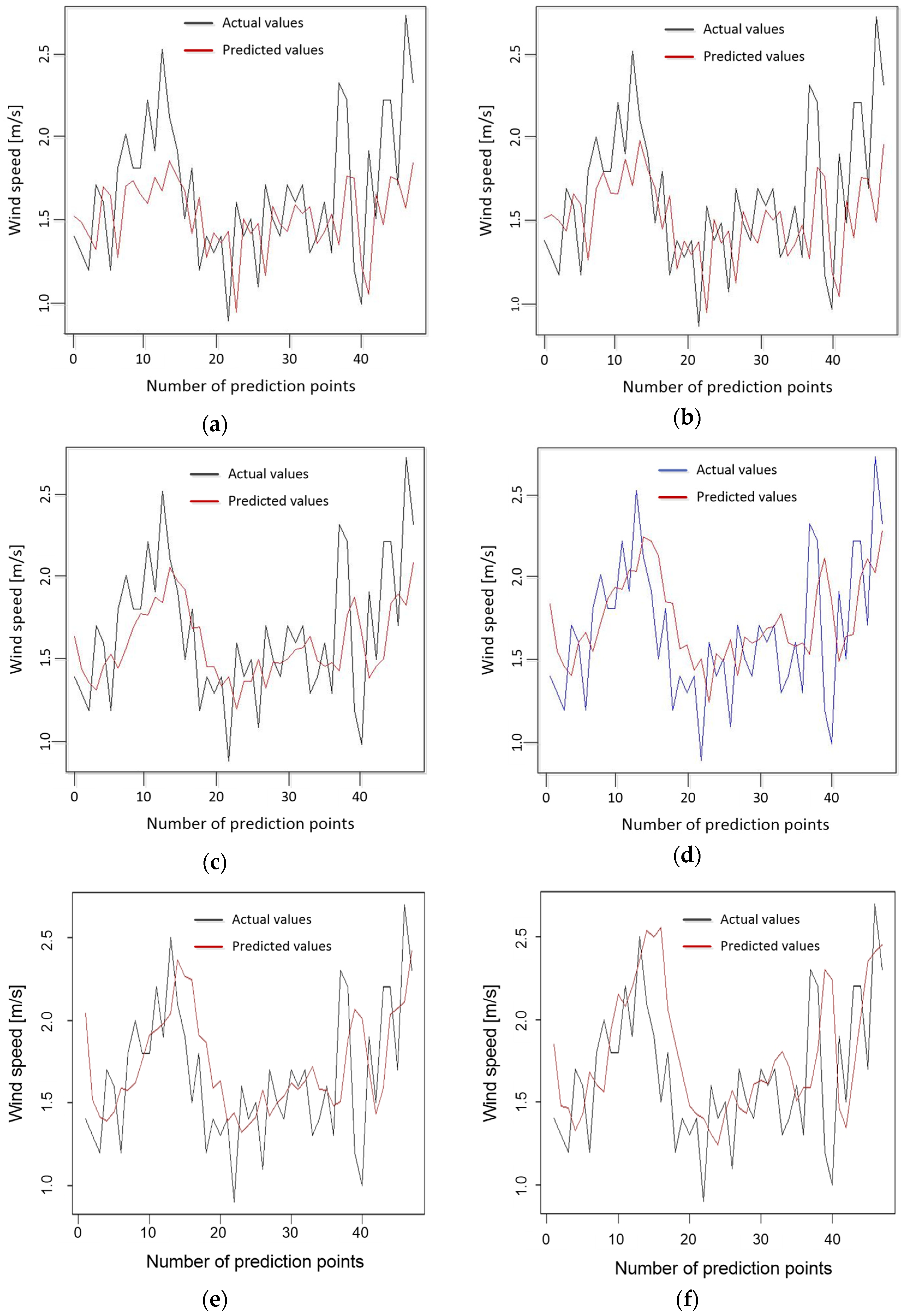
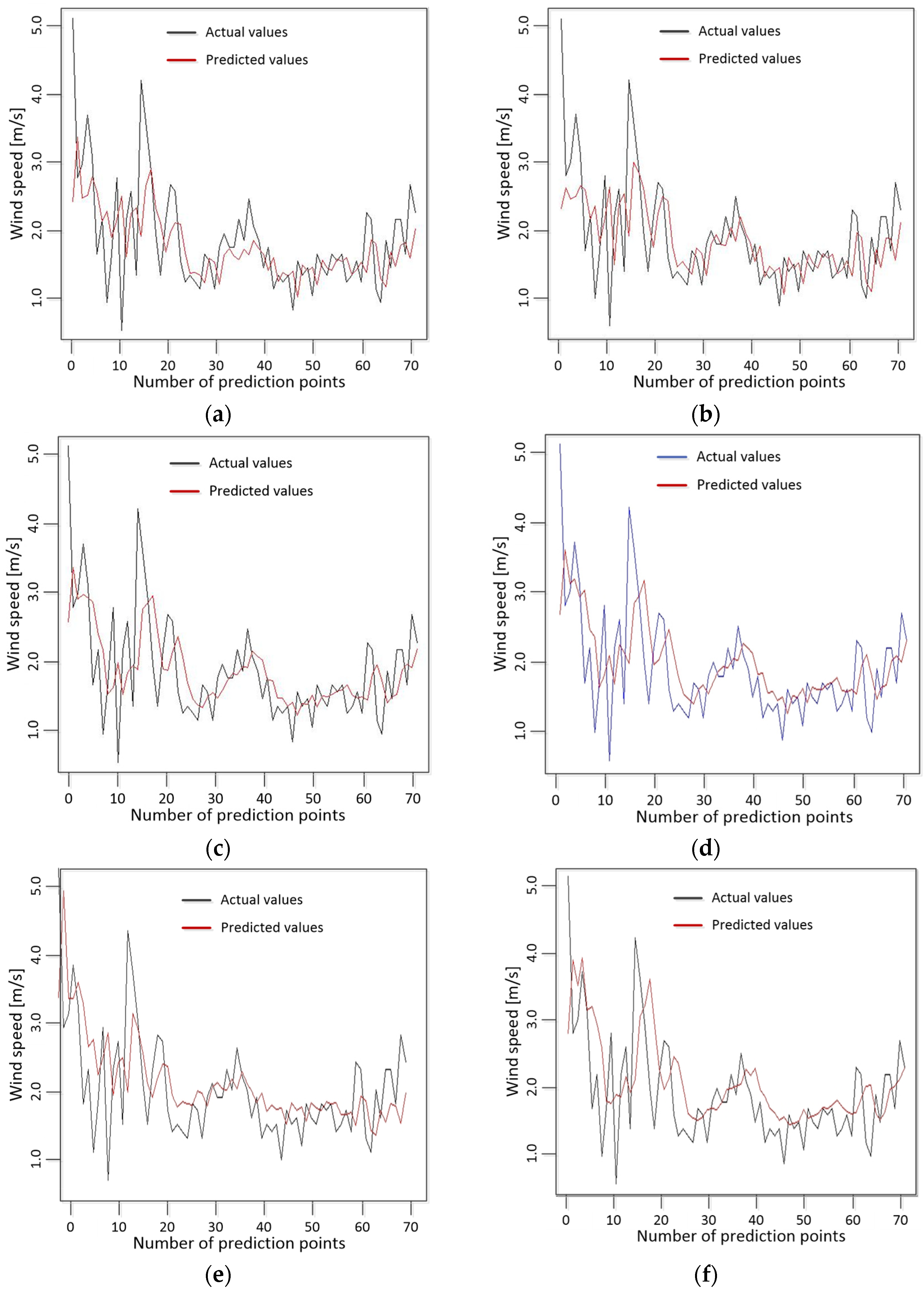
Figure 5 and Figure 6 show the prediction results for different testing models and different number of prediction points, which are grouped based on the test sequence length. Figure 5 presents the 4-h test sequence (a total of 48 prediction points with a resolution of 5 min), where graphs present the actual wind speed values as well as the predicted values. Figure 6 shows the results of the extended 6-h long test sequence (with a total of 72 prediction points and 5-min resolution). Figure 6 shows the results of the extended, 6-h long test sequence (with a total of 72 prediction points and 5-min resolution).

We can say that when there are no sudden jumps in the wind speed values (greater than 2 m/s) in the test sequence, the number of prediction points for neural network models does not affect much the prediction accuracy, so the prediction can be safely prolonged to 5 h. For the mentioned condition, the prediction accuracy is also not significantly affected by the parameters of the model function, i.e., the number of neurons in the hidden layer of the neural network.

5. Conclusions

In this paper, we have shown the analysis and testing results of the FFBP, and MLP types of neural networks, as well as the ANFIS type of fuzzy logic network, in order to investigate which type has best performance regarding the minimal absolute error and prediction duration of maximum five hours. Test results have shown that both FFBP and MLP types have similar and good performance especially when the test sequence doesn’t contain changes of wind speed larger than 2 m/s. Neural networks also outperformed the tested ANFIS fuzzy logic model.

Future work will be focused on the analysis of additional neural network models such as the generalized feed-forward neural network (GFNN) and the recursive radial basis function neural network (RRBFNN), as well as some hybrid models.