Ensemble Precipitation Estimation Using a Fuzzy Rule-Based Model ^†

Abstract

In this study, a Takagi-Sugeno (TS) fuzzy rule-based (FRB) model is used for ensembling precipitation time series. The TS FRB model takes precipitation predictions of grid-based regional climate models (RCMs) from the EUR11 domain, available from the CORDEX database, as inputs to generate ensembled precipitation time series for two meteorological stations (MSs) in the Mediterranean region of Turkey. For each MS, RCM data that are available at the closest grid to the corresponding MSs are used. To generate the fuzzy rules of the TS FRB model, the subtractive clustering algorithm (SC) is utilized. Together with the TS FRB, the simple ensemble mean approach is also applied, and the performances of these two model results and individual RCM predictions are compared. The results show that ensembled models outperform individual RCMs, for monthly precipitation, for both MSs. On the other hand, although ensemble models capture the general trend in the observations, they underestimate the peak precipitation events.

1. Introduction

Precipitation is one of the main meteorological parameters that affects water resources and it is directly influenced by climate change [1]. General circulation models (GCMs) are used to estimate precipitation under climate change [2]. However, the systematic biases between the simulated and observed values, and coarse resolution (generally a few hundred kilometers), of GCMs prevent their applications for regional-scale climate impact studies [3]. Although regional climate models (RCMs), obtained by the dynamical downscaling of GCMs, provide spatially and physically consistent outputs, with a finer resolution (typical resolution of tens of kilometers), they still have significant biases [3]. Moreover, it has long been recognized that a single model prediction does not provide the range of outcomes that are required to assess the risks of future climate change [4].

One of the alternatives to overcome the above-mentioned issues is to use an ensemble approach (EA). The EA is applied in various fields, such as biology [5], water resources [6], medicine [7], and decision-making [8]. However, the application of the EA for climate predictions is relatively new [9]. The EA is applied by [10] to assess climate change impact on hydrology and water resources. Ref. [11] assessed climate change impact on climate extremes, while [12] carried out future predictions of atmospheric rivers, by using GCMs with the EA. The EA is used by [13] to assess climate change impact on surface winds, and by [14] on extreme rainfall events as well.

Multiple linear regression (MLR) is a simple EA used to generate the superensemble, through minimization of the sum of the squares of the differences between predictors and predictands conclude that MLR has better performance skills compared to single model predictions [15,16,17]. Machine learning methods are also used for ensembling climate models. Artificial neural networks, random forest, K-nearest neighbor, and support vector machines are examples of machine learning methods for the EA that appeared in the literature [18,19,20]. In this study, another data-driven method, namely, TS FRB, identified by SC, is applied for ensembling RCM predictions.

The TS FRB model is a powerful practical engineering tool for the modeling and control of complex systems [21]. The main advantage of the TS model is that simple fuzzily defined local models will result in a nonlinear (of high order) global model [22]. The TS FRB model has wide applications in a number of fields, including adaptive nonlinear control, fault detection, performance analysis, forecasting, knowledge extraction, and behavior modeling [21]. In this study, the relation between individual RCM’s predictions and observed precipitation is represented using fuzzy rules, which are formulated through SC. Clustering is used in grouping, pattern recognition, data mining, and machine learning [23].

Fuzzy models are used for statistical downscaling of precipitation [24,25,26]; nevertheless, to the best of our knowledge, this is the first application of the TS FRB model as an EA for climate models in Turkey. The TS FRB model with one rule is equivalent to the MLR; this provides a benchmark for the evaluation of model performance in this study area. In addition to MLR, the performance of the TS FRB model is compared to that of simple ensemble mean (SEM), in terms of the prediction of monthly precipitation in the study area.

2. Methodology

2.1. Data

Daily precipitation observations from two MSs are obtained from the Turkish State Meteorological Service. One of the MSs (Afyon: MS17190) is located inland while the other (Anamur: MS17320) is located close to the shoreline (Figure 1). Observational data are subjected to a two-step quality check (QC). First, the months with more than 10 days missing data are eliminated. Then observed data is examined for the whole historical period and commonly dry months are identified as July, August, and September. Months other than these with an average precipitation less than 0.1 mm are considered unreliable and removed from the time series. For the remaining months, the monthly average time series is obtained and named as the final dataset for observations (FDO).

To build an ensemble model, monthly average precipitation simulations from eight different CORDEX RCMs are obtained for the corresponding months of FDO. RCM predictions are extracted by using the code developed by [27]. Information about the CORDEX RCMs used in this study and their long-term monthly mean and standard deviations (µ/σ) for the grid closest to the MS17190 (~17190) and MS17320 (~17230) are shown in

Table 1. RCMs used in the study.

General Circulation Models (GCM)	Regional Climate Models (RCMs)	Model Number	µ/σ (~17190)	µ/σ (~17320)
CNRM-CM5 (CNRM-CERFACS)	CCLM4-8-17	RCM1	1.85/1.20	2.89/3.38
	ALADIN53	RCM2	2.50/1.63	1.65/1.89
EC-EARTH (ICHEC)	CCLM4-8-17	RCM3	1.34/1.12	2.26/2.82
	RACMO22E	RCM4	0.95/0.71	1.52/1.75
	HIRHAM5	RCM5	1.14/0.95	2.01/2.59
CM5A-MR (IPSL)	WRF331F	RCM6	2.21/1.63	1.98/2.52
HadGEM2-ES (MOHC)	CCLM4-8-17	RCM7	1.51/1.28	3.33/3.90
	RACMO22E	RCM8	1.19/0.92	2.50/2.64

. The long-term monthly µ/σ for the observed precipitation at MS17190 and MS17320 are 1.16/0.85 and 2.88/3.45, respectively.

2.2. Takagi-Sugeno Fuzzy Rule-Based Model

In this study, a TS FRB model is developed to obtain an ensemble precipitation time series for each MS. Mathematical representation of the TS FRB model is as follows:

$$FR{B}_i^t=f\left(RC{M}_{i,1}^t,RC{M}_{i,2}^t,\dots ,RC{M}_{i,8}^t\right)$$

(1)

where $i$ is the index for the MS (here $i=1,2$), $t$ is the index for time, $FR{B}_i^t$ is the ensembled precipitation value for MS $i$ in month $t$, $RC{M}_{i,1}^t,RC{M}_{i,2}^t,\dots ,RC{M}_{i,8}^t$ are the precipitation predictions of 8 different RCMs at the grid closest to the MS $i$ in month $t$.

The rule-based structure of the TS FRB model is identified by using SC. TS FRB takes precipitation predictions of eight RCMs as inputs to predict ensembled precipitation time series at the corresponding MS as the output. In SC, together with the input data, output data is included in the clustering process. Before clustering, log-transformation is applied to all data sets and the feature space is normalized to bind all data in a unit hypercube. In SC, each data point is treated as a candidate to be a cluster center (cc), and the potential of each data point to be a cc is calculated using [28], as follows:

$$P_m={\displaystyle \sum }_{k=1}^n{e}^{-\left(4/r_a{}^2\right)\left|\right|X_m-X_k|{|}^2}$$

(2)

where $X_m$ is the normalized data point $m$, $P_m$ is the potential of the $X_m$, $r_a$ is a user-defined positive constant identifying cluster radius and $n$ is the number of data points.

The potential of a data point exponentially decays with the square of the distance between that data point and all other data points. In this way, the data points with many neighboring data have higher chances to be cluster centers. The data point having the highest potential value is assigned as the first cc. Then, the potentials are updated using [28], as follows:

$$P_m\leftarrow P_m-P_z^{*}{e}^{-\left(4/r_b{}^2\right)\left|\right|X_m-X_z^{*}|{|}^2}$$

(3)

where $X_z^{*}$ is the cc $z$, $P_z^{*}$ is the potential of the $X_z^{*}$ and $r_b$ is a user-defined positive constant. In this study, $r_b$ is taken 1.5$r_a$ to avoid cluster centers being spaced closely.

In the updating process, the potential decays exponentially with the square of the distance from each data point to the previously assigned cc. Hence, the updating process ensures the potential of data points that are close to the previously assigned cc drop significantly compared to the data points distant to it; specifically, the potential of the previous cc becomes zero. Note that the predecessor cc is used for the updating process. The data point having the highest potential after the updating process is assigned as the next cc. Updating procedure is repeated until a user-defined number of cluster centers are identified.

Each cc is, in essence, a prototypical data point that exemplifies a characteristic behavior of the dataset. Therefore, each cc can be used as the basis of a fuzzy rule that describes the system behavior [28]. To convert 9-dimensional (8 input RCMs and one output) cc to the fuzzy rules, each cc is decomposed into two vectors (first with eight and second with 1 element). In this study, each fuzzy rule has the following form:

$$\begin{array}{ll}\mathrm{Rule} a:& \mathrm{IF} x_1 \mathrm{is} M_1^a\& x_2 \mathrm{is} M_2^a \&\dots \& x_8 \mathrm{is} M_8^a \\ & \mathrm{THEN} y=N_1^a{x}_1+N_2^a{x}_2+\cdots +N_8^a{x}_8+N_9^a\end{array}$$

(4)

where $x_1, x_2,\dots ,x_8$ are the input variables and $y$ is the output variable, $M_1^a,M_2^a,\dots , M_8^a$ are antecedent fuzzy sets for rule $a$, which are defined by Gaussian membership functions and $N_1^a, N_2^a,\dots ,N_8^a, N_9^a$ are the parameters to be optimized for rule $a$. After obtaining fuzzy rules, well-known TS FRB [29] model is constructed and parameters are optimized by recursive least square estimation. For further details, the reader may refer to [28,30].

To select the best combination of the clustering parameters (e.g., the number of cc and $r_a$), a trial–error procedure is applied. Limiting the study space with 20 cc and maximum $r_a$ of 1, 400 FRB models are built using the FDO as the output and corresponding RCMs as inputs for each MSs. Dataset is randomly sampled and 75% of the dataset is used for training while the rest is used for validation. Combination resulting in the best performance in the validation set is selected and the selected number of cc and $r_a$ are used in ensembling.

The framework of the TS FRB is given in Figure 2. In the EA, 5-fold validation is used. The folds are combined together to form the validation time series (VTS) of precipitation. Note that each data point is used in the validation dataset once.

2.3. Simple Average of the Models for Ensembling

The SEM is formed to predict monthly precipitation values for the closest grid to the selected MS. Formulation of SEM is as follows [31]:

$$SE{M}_i^t={\overline{OBS}}_i+{\overline{RCM}}_i^t-{\overline{RCM}}_i$$

(5)

where $SE{M}_i^t$ is the precipitation prediction at grid $i$ in time $t$, ${\overline{OBS}}_i$ is the climatology of the precipitation observation at grid $i$, ${\overline{RCM}}_i^t$ is the average of the eight RCMs for grid $i$ at time $t$ and ${\overline{RCM}}_i$ is the climatology of the eight RCMs.

3. Results

In this section, the prediction performances of the SEM and TS FRB models are analyzed and compared for the VTS. In the clustering parameter selection process for the TS FRB, it is observed that as the number of cluster centers increases, the models tend to overfit. On the other hand, the performance of the models with relatively low numbers of cluster centers is very similar to those of the models with one cc (e.g., equivalent to the MLR). As a result of the trial-and-error procedure, for MS17190, the TS FRB model with 2 cc and $r_a$ of 0.45 is selected, while 2 cc and $r_a$ of 0.65 is selected for MS17320. Using the selected parameters, ensembling is carried out, and the VTS of each MS is formed. The performances of these models, together with those of the TS FRB model with one cluster center (e.g., MLR) and SEM, are given in

Table 2. Performance of the EA and RCM.

Meteological Stations (MS)	Criteria	Best RCM		Worst RCM		Takagi-Sugeno (TS) Fuzzy Rule-Based (FRB)	MLR	SEM
		Model	Value	Model	Value
17190	Correlation (corr)	RCM3	0.29 1	RCM2	0.12	0.40 1	0.40 1	0.40 1
	Root mean square error (RMSE)	RCM4	0.96	RCM2	2.21	0.78 1	0.80	0.85
	Percent bias (PBias)	RCM8	−2.88 1	RCM2	−116	10.16	7.16	10.34
17320	corr	RCM5	0.53	RCM2	0.26	0.65 1	0.62	0.62
	RMSE	RCM8	3.12	RCM7	3.86	2.67 1	2.81	2.81
	PBias	RCM8	3.12 1	RCM7	3.86	17.7	23.91	16.88

¹ The blods referred results of the trial-and-error procedure, for MS17190, the TS FRB model with 2 cc and $r_a$ of 0.45 is selected, while 2 cc and $r_a$ of 0.65 is selected for MS17320.

, in terms of correlation (corr), root mean square error (RMSE) and percent bias (PBias).

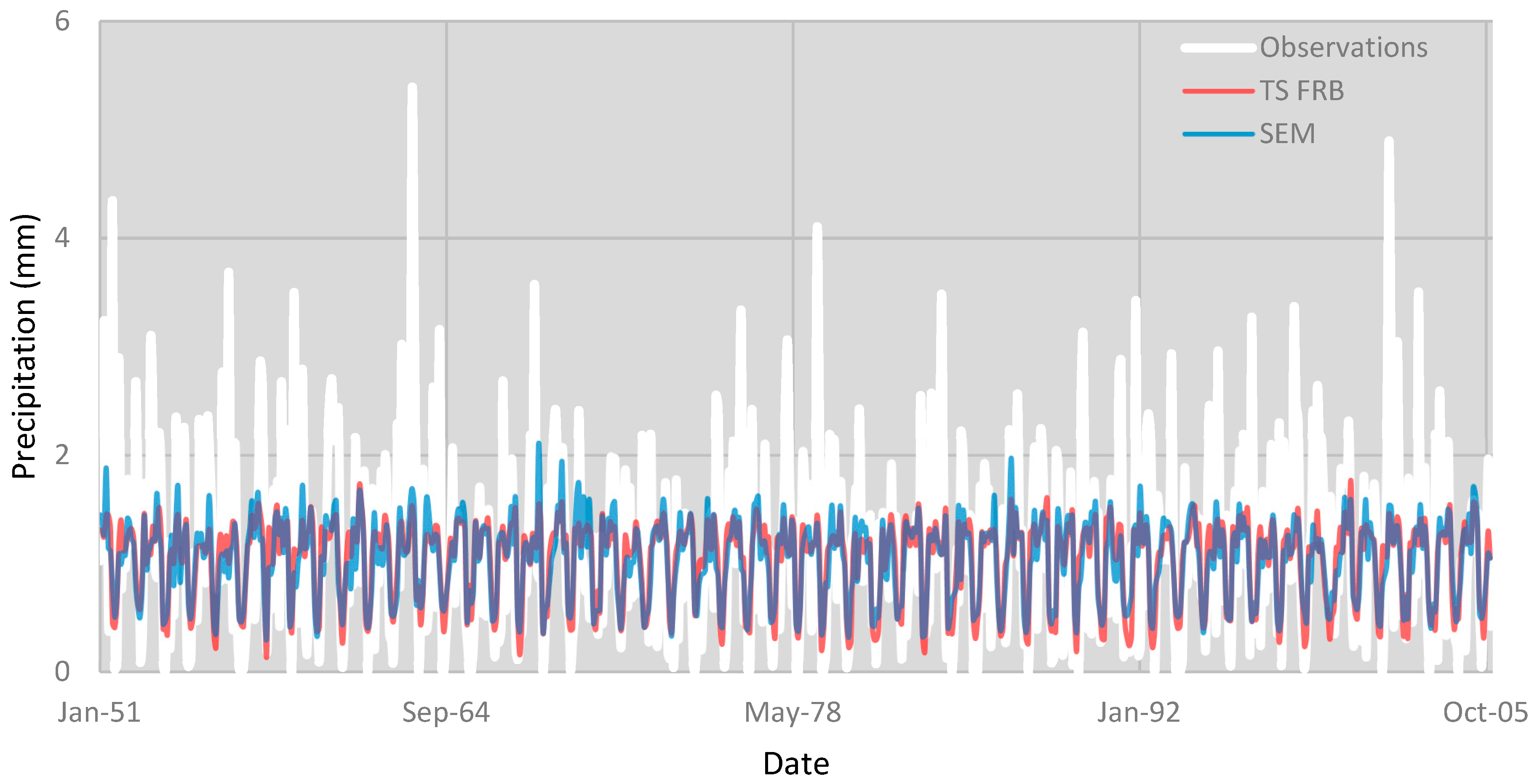
As shown in Table 2, where the best performance is given in bold, the prediction skills of TS FRB, MLR and SEM are very similar for both stations. On the other hand, the ensembled results have higher prediction skills in terms of corr and RMSE, and lower prediction skills in terms of PBias, compared to the best-performing RCM. The time series of the observations and predictions of TS FRB and SEM for MS17190 and MS17320 are given in Figure 3 and Figure 4, respectively. In Figure 3 and Figure 4, to increase visibility, transparent colors are preferred for the TS FRB and SEM predictions.

Although TS FRB and SEM follow the general trend in the observations for both MSs, both models underestimate the peak precipitations, as can be seen in Figure 3 and Figure 4. However, despite its simplicity, SEM has higher skill in the prediction of peak precipitations compared to the nonlinear TS FRB. On the other hand, although the peak precipitations for MS17320 are much larger than those of MS17190, the EAs have higher prediction skills for MS17320, especially in terms of corr.

4. Conclusions

In this study, the ensembling performance of a TS FRB model for monthly precipitations is compared to those SEM and individual RCMs.

• The analysis shows that the performance, in terms of corr and RMSE, of the EA is better, compared to the individual RCMs for both MSs. However, the PBias values of the best-performing RCM are much better than those of SEM and TS RFB;
• The nonlinear TS FRB model has very similar prediction skills to the simple SEM model. So, when the effort to select the best cc and $r_a$ combination is taken into account, SEM is more efficient, compared to the TS FRB model for ensembling;
• Both models failed to predict peak precipitation events.

References

- Trenberth, K.E. Changes in precipitation with climate change. Clim. Res. 2011, 47, 123–138. [Google Scholar] [CrossRef] [Green Version]
- Eden, J.M.; Widmann, M.; Maraun, D.; Vrac, M. Comparison of GCM-and RCM-simulated precipitation following stochastic postprocessing. J. Geophys. Res. Atmos. 2014, 119, 11-040. [Google Scholar] [CrossRef] [Green Version]
- Turco, M.; Llasat, M.C.; Herrera, S.; Gutiérrez, J.M. Bias correction and downscaling of future RCM precipitation projections using a MOS-Analog technique. J. Geophys. Res. Atmos. 2017, 122, 2631–2648. [Google Scholar] [CrossRef] [Green Version]
- Buontempo, C.; Mathison, C.; Jones, R.; Williams, K.; Wang, C.; McSweeney, C. An ensemble climate projection for Africa. Clim. Dyn. 2015, 44, 2097–2118. [Google Scholar] [CrossRef] [Green Version]
- Gårdmark, A.; Lindegren, M.; Neuenfeldt, S.; Blenckner, T.; Heikinheimo, O.; Müller-Karulis, B.; Niiranen, S.; Tomczak, M.T.; Aro, E.; Wikström, A.; et al. Biological ensemble modeling to evaluate potential futures of living marine resources. Ecol. Appl. 2013, 23, 742–754. [Google Scholar] [CrossRef]
- Choubin, B.; Moradi, E.; Golshan, M.; Adamowski, J.; Sajedi-Hosseini, F.; Mosavi, A. An ensemble prediction of flood susceptibility using multivariate discriminant analysis, classification and regression trees, and support vector machines. Sci. Total Environ. 2019, 651, 2087–2096. [Google Scholar] [CrossRef]
- Smith, T.; Ross, A.; Maire, N.; Chitnis, N.; Studer, A.; Hardy, D.; Brooks, A.; Penny, M.; Tanner, M. Ensemble Modeling of the Likely Public Health Impact of a Pre-Erythrocytic Malaria Vaccine. PLoS Med. 2012, 9, e1001157. [Google Scholar] [CrossRef] [Green Version]
- Marzocchi, W.; Taroni, M.; Selva, J. Accounting for epistemic uncertainty in PSHA: Logic tree and ensemble modeling. Bull. Seismol. Soc. Am. 2015, 105, 2151–2159. [Google Scholar] [CrossRef]
- Kotlarski, S.; Keuler, K.; Christensen, O.B.; Colette, A.; Déqué, M.; Gobiet, A.; Goergen, K.; Jacob, D.; Lüthi, D.; van Meijgaard, E.; et al. Regional climate modeling on European scales: A joint standard evaluation of the EURO-CORDEX RCM ensemble. Geosci. Model Dev. 2014, 7, 1297–1333. [Google Scholar] [CrossRef] [Green Version]
- Christensen, N.S.; Lettenmaier, D.P. A multimodel ensemble approach to assessment of climate change impacts on the hydrology and water resources of the Colorado River Basin. Hydrol. Earth Syst. Sci. 2007, 11, 1417–1434. [Google Scholar] [CrossRef] [Green Version]
- Tegegne, G.; Melesse, A.M.; Worqlul, A.W. Development of multi-model ensemble approach for enhanced assessment of impacts of climate change on climate extremes. Sci. Total Environ. 2020, 704, 135357. [Google Scholar] [CrossRef]
- Massoud, E.C.; Espinoza, V.; Guan, B.; Waliser, D.E. Global climate model ensemble approaches for future projections of atmospheric rivers. Earth’s Future 2019, 7, 1136–1151. [Google Scholar] [CrossRef] [Green Version]
- Najac, J.; Boé, J.; Terray, L. A multi-model ensemble approach for assessment of climate change impact on surface winds in France. Clim. Dyn. 2009, 32, 615–634. [Google Scholar] [CrossRef]
- Padulano, R.; Reder, A.; Rianna, G. An ensemble approach for the analysis of extreme rainfall under climate change in Naples (Italy). Hydrol. Process. 2019, 33, 2020–2036. [Google Scholar] [CrossRef]
- Krishnamurti, T.N.; Kishtawal, C.M.; LaRow, T.E.; Bachiochi, D.R.; Zhang, Z.; Williford, C.E.; Gadgil, S.; Surendran, S. Improved weather and seasonal climate forecasts from multimodel superensemble. Science 1999, 285, 1548–1550. [Google Scholar] [CrossRef] [Green Version]
- Krishnamurti, T.N.; Kishtawal, C.M.; Zhang, Z.; LaRow, T.; Bachiochi, D.; Williford, E.; Gadgil, S.; Surendran, S. Multimodel Ensemble Forecasts for Weather and Seasonal Climate. J. Clim. 2000, 13, 4196–4216. [Google Scholar] [CrossRef]
- Yun, W.T.; Stefanova, L.; Mitra, A.K.; Vijaya Kumar, T.S.V.; Dewar, W.; Krishnamurti, T.N. A multi-model superensemble algorithm for seasonal climate prediction using DEMETER forecasts. Tellus A Dyn. Meteorol. Oceanogr. 2005, 57, 280–289. [Google Scholar] [CrossRef]
- Okkan, U.; Inan, G. Statistical downscaling of monthly reservoir inflows for Kemer watershed in Turkey: Use of machine learning methods, multiple GCMs and emission scenarios. Int. J. Climatol. 2015, 35, 3274–3295. [Google Scholar] [CrossRef]
- Wang, B.; Zheng, L.; Liu, D.L.; Ji, F.; Clark, A.; Yu, Q. Using multi-model ensembles of CMIP5 global climate models to reproduce observed monthly rainfall and temperature with machine learning methods in Australia. Int. J. Climatol. 2018, 38, 4891–4902. [Google Scholar] [CrossRef]
- Ahmed, K.; Sachindra, D.A.; Shahid, S.; Iqbal, Z.; Nawaz, N.; Khan, N. Multi-model ensemble predictions of precipitation and temperature using machine learning algorithms. Atmos. Res. 2020, 236, 104806. [Google Scholar] [CrossRef]
- Angelov, P.P.; Filev, D.P. An approach to online identification of Takagi-Sugeno fuzzy models. IEEE Trans. Syst. Manand Cybern. Part B 2004, 34, 484–498. [Google Scholar] [CrossRef] [PubMed] [Green Version]
- Angelov, P. An approach for fuzzy rule-base adaptation using on-line clustering. Int. J. Approx. Reason. 2004, 35, 275–289. [Google Scholar] [CrossRef]
- Jain, A.K.; Murty, M.N.; Flynn, P.J. Data clustering: A review. ACM Comput. Surv. 1999, 31, 264–323. [Google Scholar] [CrossRef]
- Najafi, M.R.; Moradkhani, H.; Wherry, S.A. Statistical downscaling of precipitation using machine learning with optimal predictor selection. J. Hydrol. Eng. 2011, 16, 650–664. [Google Scholar] [CrossRef]
- Wetterhall, F.; Bárdossy, A.; Chen, D.; Halldin, S.; Xu, C.Y. Statistical downscaling of daily precipitation over Sweden using GCM output. Theor. Appl. Climatol. 2009, 96, 95–103. [Google Scholar] [CrossRef]
- Bárdossy, A.; Pegram, G. Downscaling precipitation using regional climate models and circulation patterns toward hydrology. Water Resour. Res. 2011, 4. [Google Scholar] [CrossRef]
- Kentel, E.; Akgun, O.B.; Mesta, B. User-Friendly R-Code for Data Extraction from CMIP6 outputs. In AGU Fall Meeting Abstracts; PA33C-1098; American Geophysical Union: Washington, DC, USA, 2019. [Google Scholar]
- Chiu, S.L. Fuzzy model identification based on cluster estimation. J. Intell. Fuzzy Syst. 1994, 2, 267–278. [Google Scholar] [CrossRef]
- Takagi, T.; Sugeno, M. Fuzzy identification of systems and its applications to modeling and control. IEEE Trans. Syst. Man Cybern. 1985, 1, 116–132. [Google Scholar] [CrossRef]
- Mesta, B.; Akgun, O.B.; Kentel, E. Alternative solutions for long missing streamflow data for sustainable water resources management. Int. J. Water Resour. Dev. 2020, 1–24. [Google Scholar] [CrossRef]
- Cane, D.; Milelli, M. Multimodel SuperEnsemble technique for quantitative precipitation forecasts in Piemonte region. Nat. Hazards Earth Syst. Sci. 2010, 10, 265–273. [Google Scholar] [CrossRef]
Figure 1.
Study area and the location of the meteorological stations (MSs).
Figure 2.
Framework of the ensemble Takagi-Sugeno (TS) fuzzy rule-based (FRB).
Figure 3.
Time series of VTS obtained from TS FRB and simple ensemble mean (SEM) for MS17190.
Figure 4.
Time series of VTS obtained from TS FRB and SEM for MS17320.