Review of Deterministic and Probabilistic Wind Power Forecasting: Models, Methods, and Future Research


School of Electrical and Computer Engineering, National Technical University of Athens (NTUA), 15780 Athens, Greece
*
Author to whom correspondence should be addressed.
Electricity 2021, 2(1), 13-47; https://0-doi-org.brum.beds.ac.uk/10.3390/electricity2010002
Submission received: 5 October 2020
/
Revised: 17 November 2020
/
Accepted: 14 December 2020
/
Published: 8 January 2021
Abstract
:The need to turn to more environmentally friendly sources of energy has led energy systems to focus on renewable sources of energy. Wind power has been a widely used source of green energy. However, the wind’s stochastic and unpredictable behavior has created several challenges to the operation and stability of energy systems. Forecasting models have been developed and excessively used in recent decades in order to deal with these challenges. Deterministic forecasting models have been the main focus of researchers and are still being developed in order to improve their accuracy. Furthermore, in recent years, in order to observe and study the uncertainty of forecasts, probabilistic forecasting models have been developed in order to give a wider view of the possible prediction outcomes. Advanced probabilistic and deterministic forecasting models could be used in order to facilitate the energy systems operation and energy markets management. This paper introduces an overview of state-of-the-art wind power deterministic and probabilistic models, developing a comparative evaluation between the different models reviewed, identifying their advantages and disadvantages, classifying and analyzing current and future research directions in this area.
1. Introduction
Global climatic conditions have changed rapidly over the last decades. The continuous increase of energy needs all over the world, as well as the use of limited reserves of traditional energy resources (coal, oil, and natural gas), have turned the interest of researchers towards renewable energy. One of the most important and widely used renewable resources is wind power, thanks to its widely distributed nature [1]. Considering the advance in technology and research, wind power has become an indispensable part of the global energy system and it could be possible that in the future it could largely replace conventional energy resources used for power generation.
Because of the wind’s stochastic nature and intermittence, the increased penetration of wind power has created many challenges in the operation and planning of power systems worldwide [1]. To deal with these challenges, it has been necessary to develop wind power forecasting models and methods with increased accuracy. As a result, wind power forecasting has been researched and developed over the past decades in order to deal with the challenges that arose with the rapid increase in the use of wind power in the power systems worldwide. Forecasting models not only forecast wind power, but also help stabilize power systems and organize electricity markets [2].
Deterministic forecasting models have been used over the last decades in wind power generation and play an important role in the daily operation of power systems. Given a set of input data, deterministic forecasting models are able to provide the user with a single-valued expectation series of the wind power output. Depending on the evaluation of the model used and its errors, the user is able to use the model’s results to estimate the closest possible output of wind power generation. For this, numerous deterministic forecasting models have been proposed and developed to predict as accurately as possible the wind power output. Naturally, such models, thanks to the development of technology, are still improving in order to provide better forecasts [3].
Over the last decade, probabilistic forecasting has been the center of attention for researchers since, unlike deterministic forecasting, probabilistic forecasts give important information over the uncertainty of the forecasts. While deterministic methods give single-valued results of wind power generation, probabilistic methods give a wider view of possible wind power outputs since the output of such models could be quantiles, prediction intervals (PIs), and distributions. In this way, the user has a better view of the possible forecast compared to the single-value output of a conventional deterministic model. As a result, it could be possible in the future that probabilistic forecasts could be used effectively in decision-making problems, transforming various decision-making activities to probabilistic, such as wind power trading in electricity markets [4], optimal power flow [5], and unit commitment [6].
Evaluation is a very important aspect of wind power forecasting. Evaluating proposed forecasting models allows a constant comparison between different models and consequently their constant development. Evaluation is important in both deterministic and probabilistic forecasts. In deterministic forecasting, simple comparative measures have been used over the years to evaluate the performance of the forecasting models. However, evaluating probabilistic forecasts is more complicated than evaluating point predictions. While in the point forecasts the evaluation is based on the deviation between predicted and measured power values, the same is not possible in probabilistic forecasting since such a comparison is not possible directly. This is why defining a framework to evaluate probabilistic forecasts has been researched a lot over the past years.
With the increased importance of wind power in energy systems, more and more researchers not only intend to create new advanced models, but also observe the function of existing models in various cases. Recently, review works have studied deterministic and probabilistic forecasting models in order to comprehend the methodologies used in wind power forecasting as well as determine possible development possibilities in the future. More specifically, [7] divided the deterministic forecasting methods reviewed in four categories and presented their different characteristics. In [8], an in-depth review of wind power forecasting methods was presented as well as an overview of benchmark techniques and uncertainty analysis. The review works [9,10] classified the reviewed deterministic forecasting works from the perspective of forecasting horizons and time scales. In [11], various works were reviewed and the forecasting accuracy of the models based on the variable factors used in the forecast was discussed. The work [12] reviewed state-of-the-art probabilistic forecasting models and presented an overall framework of probabilistic forecasting evaluation. The work [13] presented the fundamental concepts of state-of-the-art probabilistic methodologies. The work [14] focused on the principals and features of state-of-the-art wind power forecasting uncertainty analysis.
The above bibliography review shows that the majority of the review papers are focused on presenting the state-of-the-art methodologies of either deterministic or probabilistic wind power forecasting. However, there is no review work focused on presenting evaluation results in order to propose a comparative knowledge between different methodologies in specific conditions.
The contributions of this review paper are manifold:
- It offers a unique and wider view by reviewing the state of the art in both the deterministic and probabilistic wind power forecasting methodologies and by identifying their advantages and disadvantages.
- It provides comparative results among the models of the reviewed works, based on evaluation measures.
- It proposes future research goals of deterministic and probabilistic forecasting models, not only to improve the methodologies used in forecasting, but also to make both deterministic and probabilistic forecasting models more useful and helpful in energy markets and power systems.
- It aims to help researchers in having a view of possible expectations in research cases corresponding to the ones compared in the paper.
The structure of the paper is as follows. Section 2 analyzes the evaluation methods used for assessing the deterministic and probabilistic forecasting methodologies. Section 3 analyzes state-of-the-art wind power deterministic forecasting methodologies. Section 4 describes state-of-the-art wind power probabilistic forecasting methodologies. Section 5 analyzes recent wind power forecasting methodologies. Section 6 provides the advantages and disadvantages of using wind power deterministic and probabilistic forecasting methods. Section 7 identifies the core contribution of the reviewed works for wind power deterministic and probabilistic forecasting methods. Section 8 presents the comparative results between the methodologies compared in the reviewed works. Section 9 proposes future research directions and possibilities. Section 10 summarizes the main findings and concludes the paper.
2. Evaluation of Wind Power Forecasts
Evaluating a forecasting model is of core importance to comprehending its quality and accuracy. The continuous need to improve existing forecasting models and develop new ones, calls for a way to compare such models concerning the accuracy of their results. In deterministic forecasting as well as in probabilistic forecasting, different ways of comparing and evaluating different models have been used throughout the years.
2.1. Deterministic Forecasting
There are different ways to evaluate deterministic models. Evaluation of the models is an important procedure, since it allows the comparison between different models, highlights possible problems in the methodologies used, and guides possible improvements. Furthermore, the evaluation of deterministic models is quite easy to use and understand, as it consists of simple error metrics that can be easily compared between different models. Such error metrics include:
- Mean Absolute Error (MAE)
- Mean Squared Error (MSE)
- Root Mean Squared Error (RMSE)
As described in (1), MAE is the average value of the absolute error of the N forecasted error values en.
MSE is the average value of the squared error, which is the squared difference between the actual and predicted values. It can be described as:
As described in (3), RMSE represents the squared root of the quadratic mean of the difference between the actual and predicted values:
2.2. Probabilistic Forecasting
Evaluating wind power probabilistic forecasts is not that simple. While in deterministic forecasting the evaluation takes place by comparing simple error metrics, in probabilistic forecasting the evaluation is a more complicated process. Considering the fact that wind power generation itself is a complex process, the uncertainty of the probabilistic forecasting models is influenced by a large number of external factors.
The properties needed to evaluate probabilistic predictions are reliability, sharpness, resolution and skill score. Reliability is usually the first parameter that should be evaluated. Since non-parametric probabilistic predictions include a single quantile forecast, or a collection of quantile forecasts, the evaluation of their reliability is based on verifying the reliability of each one of those quantile forecasts. A critical measure that is widely used is the Prediction Interval Coverage Probability (PICP):
where Ntest is the number of the test samples used, and ci is the PICP’s indicator that is defined as:
where ti is the measured target and Lt and Ut are the lower and upper bounds of the prediction interval, respectively.
PICP is directly connected and compared to the Prediction Interval Nominal Coverage (PINC) percentage, presented in (6):
where (1 − α) expresses the nominal coverage probability of the prediction intervals. The closer the PICP is to the PINC the more reliable is the PI. Another simple metric usually used is the Average Coverage Error (ACE):
The closer the ACE value is to zero, the higher the reliability of the PI.
Sharpness refers to the width of the prediction intervals derived from the forecasting process. A narrower PI is generally preferred over a wider one, since it narrows down the possible outcomes of the forecast and therefore offers better information to the user, facilitating decision making. A common measure used to estimate and control the PI’s width is the PI Normalized Average Width (PINAW), defined as:
where R is the range of the underlying targets that were used for normalizing PIs.
The PI Normalized Root-mean-square Width (PINRW) is also used and is defined as:
Another measure that is widely used is the Coverage Width Criterion (CWC), which simultaneously defines both the reliability and the sharpness of a PI. CWC is calculated by (10):
where μ is the confidence level and it usually equals 1 − α; η is a penalty coefficient used to increase the difference between PICP and μ whenever PICP is smaller than μ; and γ(PICP,μ) is defined as follows:
The resolution refers to the ability of a forecasting model to generate different probabilistic information according to the forecast conditions and to provide reliable and accurate forecasting distributions.
Skill score is another important evaluation property that allows the comparison between different predictive approaches, since a higher overall skill score suggests a higher skill of the proposed probabilistic forecasting model over other predictive models.
The use of the above evaluation tools (a) allows the evaluation of a specific wind power probabilistic forecasting (WPPF) model; (b) allows the comparison of a model with other WPPF models; and (c) may identify possible problems in aWPPF model that is under development and evaluation. As a result, WPPF models can keep improving their accuracy and performance and also become simpler for the user to understand.
3. Wind Power Deterministic Forecasting
3.1. Physical Approach
The physical approach is based on atmospheric conditions and uses actual meteorological data to create a prediction model. Such models use topographical data, like the height at which the wind farm is located, the surface’s roughness, obstacles, as well as meteorological data, like local temperature, humidity, pressure, wind speed, and direction. The Numerical Weather Prediction (NWP) model is the most typical physical approach and uses such data in order to estimate an accurate value of wind speed for each turbine of a wind park in order to forecast wind power output as accurately as possible.
NWP models use hydrodynamic and thermodynamic models of the atmosphere in order to make weather-based predictions over specific initial-value and boundary conditions. Various global and regional NWP forecasting models have been developed over the years [15]. Basically, those NWP forecasting models operate by solving complex mathematical models, which are based on weather data (i.e., temperature, humidity, etc.). Such models demand lots of computations and therefore are more reliable for long-term forecasts [9].
NWP models attempt to focus on the evolution of the atmosphere at its specific scale, despite the fact that high spatial resolution cannot be combined with temporal resolution. NWP with high spatial resolution has low temporal validity for its predictions, while NWP with low spatial resolution has greater temporal validity. Predictions of NWP models with lower temporal validity are used for short-term wind power forecasting [16].
One of the main disadvantages of physical approaches is collecting local terrain data since many times the terrain can be really complex. Furthermore, since NWP models are highly complex models, they require high computation time. As a result, in order to improve the accuracy of the models, higher computation time is required as well as higher cost. Finally, the predictive accuracy of physical approaches is connected with the stability of the weather conditions of the area that is being researched. Since wind speed is one of the most important parameters in these models, it is expected that stable weather conditions give more accurate NWP and as a result more accurate wind power predictions, while unstable weather conditions give more inaccurate results.
3.2. Statistical Approach
Statistical approaches are based on the correlations between the explanatory variables used and the targets of the model in order to make accurate predictions. Statistical methods are based on either time series models or artificial intelligence (AI) models. Table 1 presents a classification of the statistical approaches used for wind power deterministic forecasting.
3.2.1. Statistical Approaches Based on Time Series
The most popular model of time series-based statistical approach is the Auto Regressive Moving Average (ARMA) model in wind power forecasting. A widely used extension of the ARMA model is the Auto Regressive Integrated Moving Average (ARIMA) model. Other statistical approaches based on time series are the persistence method and grey prediction.
ARMA and ARIMA
The ARMA model, as proposed in [17], is a combination of the Autoregressive (AR) model and the Moving Average (MA) model and can predict future values of a time series through the linear regression of already observed values of said time series. A typical ARMA(p,q) model can be described as:
where Xt represents the time series value for time t, φi is the autoregressive parameter, θi is the moving average parameter and at is the normal white noise. The model in (12) can either contain the autoregressive part AR(p), or the moving average part MA(q), or both parts ARMA(p,q). The AR part is responsible for the previously observed wind power values whereas the MA part is responsible for previous errors of the model in order to improve the final prediction [18].
The main disadvantage of this model is that it requires a lot of high-quality stationary historical data in order to be accurate. However, most of the time, the data is non-stationary, and as a result, further measures need to be implemented in order to achieve a good predictive result.
To deal with the non-stationary data problem of the ARMA model, a type of differential transformation is used. The original time series is differenced in order to achieve the stationarity of the data [19]. As a result, the model is called Auto Regressive Integrated Moving Average (ARIMA(p,d,q)) when the integration part is implemented. The I(d) part is responsible for the number of the differencing times of the original time series. To achieve stationarity, the differenced time series can be described as:
where Xt is the original time series and Yt is the new one after the differential transformation for the order d = 1, since it was differenced one time.
In [20], the ARMA model is compared to the performance of an Artificial Neural Network (ANN) model. The two models were used in three different case studies in order to be evaluated efficiently. The first case study was for a one-hour-ahead wind speed forecast study, the second was for a wind speed forecasting study in order to support bidding decisions in the Iberian Electricity Market, and the third was for an one-hour-ahead wind power forecast study. Based on the results of the three case studies, the ARMA model had a generally better performance, while the ANN model had a better processing time. However, it was emphasized that the processing time could pose an importance decision factor depending on the application the user is interested in researching.
The work [21] used a combination of the ARMA model for forecasting for the next few minutes to a maximum of one hour, and the pattern-matching method for forecasting for the next one to six hours. By using wind power values as input data, the model aimed for ultra-short-term forecasting in order to support the power dispatcher in real-time monitoring. While the ARMA model had better accuracy in shorter time scales, with the time scale getting longer, pattern-matching method was found to be getting more accurate results. Furthermore, it was proposed that a hybrid ARMA-pattern-matching model should be further researched at longer time scales.
In [22], ARMA models were researched to improve persistence forecasts. Data from two different cases, Lake Benton and Storm Lake, were used in the study. Various alternative ARMA models were used for up to six hours forecasting horizon. It was found that the ARMA (1,24) had the best performance of all the models tested. Furthermore, it was observed that for greater forecasting horizons, the accuracy of the models decreased significantly. The proposed ARMA models managed to surpass the persistence model in most cases compared. However, there were cases were the RMSE did not decrease significantly when compared to that of the persistence model.
In [23], ARMA models, along with the wavelet transform (WT), were used for wind speed prediction. The model used wind speed data, where the time series had a total of 120 points taking one sample per hour. The wind speed time series was firstly decomposed with a wavelet transform process picking up the low frequency gentle signals. It was concluded that this process improved significantly the accuracy compared to using the simple time series. Afterwards, the ARMA model was used for the prediction process.
In [24], an ARIMA model was used in combination with an Autoregressive Conditional Heteroscedasticity (ARCH) model in order to improve the traditional ARIMA model’s accuracy. Firstly, the ARIMA model was constructed based on wind speed data. However, the residuals acquired after the ARIMA process were not related. To deal with this problem, a Generalized Autoregressive Conditional Heteroscedasticity (GARCH) model was used to fit the residuals derived from the ARIMA model. The Mean Relative Error (MRE) was used to evaluate the results of the ARIMA and the ARIMA-GARCH model and it was found that the proposed model’s MRE reduced significantly to 11.2% in comparison with 17.4% of the ARIMA model. To further improve the proposed model, the influence of atmospheric factors was proposed as a future research.
In [25], the suitability of fractional-ARIMA (f-ARIMA) model is investigated in order to obtain more accurate next hour wind speed predictions. The f-ARIMA model is chosen in this case due to its slow decay in its autocorrelation function, which makes it an interesting tool when using data that pose long range correlations. The forecast was processed by the proposed f-ARIMA model, the ARIMA model and the persistence model. The evaluation of the results of the wind speed forecasts, which was based on the Daily Mean Error (DME), the variance (σ2) and the square root of the Forecast Mean Square Error, showed that the proposed model was overall more accurate in comparison with the other two models. The impact of wind speed forecasts on wind power forecasts was studied. Via the power curve of a specific wind turbine generator, the wind speed data were used to map corresponding wind power data through cubic interpolation. The results have shown that when the wind speed excursions were small, the persistence model gave smaller errors than the f-ARIMA model. However, when the wind speed excursions were bigger, the ARIMA model proved to be more stable and gave more accurate results.
Grey Prediction Method
The grey prediction method, as proposed in [26], was developed to deal with problems characterized by uncertainty, where there is a significant lack of information and data [27]. According to [28], the grey prediction method is a useful tool for sample modeling using insufficient information due to its efficiency when used in uncertain systems. However, at longer time scales it has proved to be highly inaccurate, so it has only been used for very-short-term predictions.
3.2.2. Statistical Approaches Based on Artificial Intelligence
Artificial Neural Network
The most well-known models to be used in statistical approaches based on AI are artificial neural networks. The whole idea of ANNs was inspired by the biological neurons of a human brain. The whole function of the ANNs is the evaluation of the input data given and the continuous re-evaluation of these data and new trained data, in order to achieve an accurate predictive result, exactly like a human brain evaluates data.
A typical ANN consists of an input layer, where the historical data are implemented, an output layer, where the point forecasted values are provided, and one or more hidden layers, where the evaluation of the data from the input layer and the output layer takes place. Each layer consists of neurons connected to the ones of the previous layer. Each connection between neurons has a specific weight that highlights the importance of this connection and is the key to achieve the best possible prediction accuracy. The Neural Network (NN) is finally trained in order to get the optimal weight values of each connection and give the best possible output values.
In [29], the performance of three different conventional NNs was compared. Those NN models were the Feed Forward Back-Propagation (FFBP), the Radial Basis Function (RBF) and the Adaptive Linear Element (ADALINE) models. Wind speed data from two different sites were used. The evaluation of the models was based on MAE, mean absolute percentage error (MAPE), and RMSE evaluation metrics. It was concluded that the accuracy of the researched NNs could differ according to the inputs used or the learning rate. Furthermore, it was proposed that the selection of a NN should be decided according to the needs of the research and the data. As a result, it was concluded that a NN model should be selected after a trial-and-error process.
The work [30] used different ANN models for short term wind speed forecasting. A different model was developed for each month of the year. Four different configuration models were tested, two of them with two layers and the other two with three layers. Based on the evaluation of the models using the MSE and MAE, the fourth model that had two layers with two input neurons and one output neuron had the best accuracy, with a MSE value of 0.0016 and a MAE value of 0.0399.
In [31], an ANN model was used for short-term wind power forecasting. More specifically, a three-layered feed-forward NN was proposed for the forecasts. The Levenberg-Marquardt algorithm was used for the NN’s training process in order for the training to be faster. Based on the evaluation of the proposed model, an average MAPE of 7.26% was achieved while the corresponding MAPE value of the persistence model was 19.05%. Moreover, the computational time of the model was less than 5 s. As a result, the proposed ANN model is accurate and fast.
In [32], a NN model along with fuzzy logic was proposed for wind power forecasting. NWP data as well as data from the supervisory control and data acquisition system were used as input. Thanks to their adaptive nature, fuzzy NNs are able to adapt their parameters in case of changes in the function of the wind farm. According to the RMSE values of specific representative dates, which were less than 15%, the proposed model had efficient forecasting accuracy and was suitable for short-term forecasting.
The work [33] proposed a Convolutional Long Short-Term Memory (Conv-LSTM) network for short-term WPF. Before the application of the Conv-LSTM, the Variational Mode Decomposition (VMD) was used in order to eliminate any non-stationary features of the raw data. Afterwards, the Conv-LSTM is implemented for the preliminary prediction results as well as to extract spatio-temporal information of the forecasting sub-series. The efficiency of the proposed model was tested in two different experiments. In the first experiment, only two turbines were taken into account for the forecasting. The proposed model was compared to other seven models for three different time scales (15 min, 30 min, 1 h). For both turbines, based on the MRE, MAE, MSE and RMSE error metrics, the proposed model gave significantly better results than the other models. In the second experiment, two wind farms were taken into account for the forecasting. The proposed model was again compared to other seven models for three different time scales (15 min, 30 min, 1 h). For both wind farms, based on the MRE, MAE, MSE and RMSE error metrics, the proposed model outperformed the other models.
Support Vector Machine
Support vector machine (SVM) [34] is another model of artificial intelligence that has been widely used in wind power forecasting. SVMs can basically map a set of data into a high dimensional feature space through a nonlinear mapping process in order to proceed with the linear regression, thus simplifying a really complex process [35,36]. As a result, it is a great tool for classification as well as regression and prediction.
In [35], an SVM-based model was used to firstly predict the wind speed values, which were subsequently used to forecast the wind power values based on the power-speed characteristics of the wind turbine generators. The proposed model was compared to the persistence model and an RBF-NN model for very-short-term forecasting (less than 6 h) and short-term forecasting. For the very-short-term forecasts, the resolution of the data samples was set to one hour. The effectiveness of the proposed model was also researched, investigating the number of days for which it would give accurate results and was found that the limit was 10 days, since after 10 days the MAPE increases significantly. For the short-term forecasts, the resolution of the data samples was set to two hours. For up to 16 h, the results of the SVM model and the RBF-NN were accurate and better than the persistence model, with the proposed SVM model always having a better skill score. In the final comparison of the models, the SVM model posed a skill score of more than 26% even at 16 h forecast horizon and outperformed the other models. However, for bigger forecast horizons, the proposed model gave poor results and further atmospheric data or NWP were proposed for improving the model’s accuracy in the future.
In [37], two SVM models were proposed and compared in order to optimize prediction precision and calculation speed. The first model combined SVM and the wavelet transform, while the second model combined SVM and RBF. Based on the results, the first model had better accuracy overall for all the time scales tested and also better calculation speed. Thanks to the wavelet transform used in the WT-SVM model, the model did not have to deal with the original complex wind data and the whole process was simplified and thus had better results than the RBF-SVM model.
The work [38] used SVM for wind speed simulation after using wavelet transform to decompose the original wind speed signal into an approximation signal and a detail signal. Afterwards, the SVM model is responsible for the training process. The input data used were the wavelet transform outputs and temperature. The training and validation error were optimized with the genetic algorithm (GA). The new optimized model was used for the final prediction. Based on the MAE and MAPE results, the proposed WT-SVM-GA model managed to outperform both the persistence and the single SVM-GA models.
In the work [39], an SVM-based model was proposed for short-term WPF. The Improved Dragonfly Algorithm (IDA) was used in order to estimate the optimal parameters to improve the SVM model’s performance. The proposed IDA-SVM model was compared to several models, the majority of which were SVM models that used different optimization algorithms, as well as a simple Back Propagation Neural Network (BPNN) and the Gaussian Process Regression (GPR). Based on the NRMSE, NMAE, MAPE and R2 error metrics, the proposed IDA-SVM model managed to outperform the other models for both winter and autumn datasets.
3.3. Hybrid Approach
Due to the development in the technologies used in wind power forecasting, hybrid methods are being used more and more in order to achieve better forecasting results. Hybrid approaches aim to use the advantages of the combined models used in order to achieve an optimal performance. The models combined could be physical and statistical models, models for different time scales (for example, short-term models and medium-term models), or different statistical models.
In [40], a novel hybrid method based on wavelet transform and ANN was proposed to provide short-term wind power forecasts that outperformed various conventional models. The model’s process started with the wavelet transform decomposing the wind power signal in approximations and details. Afterwards, the WT outputs would be used as input and be trained with a NN, and subsequently, with the inverse WT, the NN’s outputs would be reconstructed to give the forecasted wind power time series. The model used only historical data as input. Compared to the persistence model, the ARIMA model and a single-NN model, the proposed method gave a significantly better MAPE result with an average value of 6.97%, while its computation time was less than 10 s.
The work [41] proposed two different hybrid models, ARIMA-ANN and ARIMA-SVM, for wind power and wind speed time series forecasting. In the first model, the ANN used the residuals of the ARIMA process in wind speed as well as wind power forecasting. Concerning the second model, the SVM model used the residuals of the ARIMA process. In both models, it was shown that as the prediction horizon increased, the MAE increased as well. It was also concluded that the proposed models, in most forecasting time horizons tested, gave better results than ARIMA, single-ANN and single-SVM models. However, it was highlighted that in cases where the ARIMA model already gave better results compared to ANN and SVM models, using hybrid ARIMA methods did not necessarily improve the model’s performance. Furthermore, it was observed that in wind speed forecasting, there were cases where the ARIMA model had better results than the proposed hybrid models, while in wind power forecasting, there were cases where the single ANN and SVM models outperformed the hybrid models.
In [42], a hybrid model based on the empirical mode decomposition (EMD) and the SVM was proposed to reduce the effects of the non-stationarity of wind power. The basic idea of the model was to decompose the original wind power data with the EMD into intrinsic mode functions (IMF) and a residual component. Then, the training process was carried out by the SVM, using the derived IMF and the residual component. The forecasting model was created based on the optimal kernel functions used. Thanks to the decomposed time series, the model was able to function with more stable data, and compared to the single-SVM model, which finally had an RMS error of 35.40%, managed to achieve an RMS error of 15.63%.
In [43], different hybrid models based on ARIMA and ANN were proposed for wind speed forecasting of three different regions. The ARIMA model was firstly used for the wind speed forecasting. Due to ARIMA being a linear model, an ANN was used in order to deal with the non-linearity of the data values. Based on the evaluation errors (MSE and MAE) in all three regions, the hybrid model was found more accurate than the single-ARIMA model or the single-ANN model.
The work [44] proposed a hybrid model for wind power forecasting based on Bagging NNs (BaNN) combined with K-means clustering. An improved Empirical Mode Decomposition (IEMD) algorithm was introduced for the data decomposition. Furthermore, the Chaotic Binary Shark Smell Optimization (ChB-SSO) was used for the optimization of the results as well as the tuning of the BaNN parameters. The effectiveness of the proposed model was tested in three different case studies where it was compared with several different models. In the first case study of the Sotavento wind farm, the proposed model was tested for data of different months and different training periods. In all cases, based on error metrics like RMSE, NRMSE, MAPE and MMAPE, the proposed model significantly outperformed the other models. In the second case study of the Alberta wind farms, the proposed model was tested for data of different seasons as well as specific months. According to error metrics like MAPE, NMAE and NRMSE, the proposed model gave the best results in all cases when compared to other models. In the third case study of the Blue Canyon wind farm, the proposed model was tested for different forecasting horizons with data from a specific month. According to the error metrics of NMAE and NRMSE, the proposed model significantly outperformed the other models.
In the work [45], a hybrid Long Short-Term Memory (LSTM) neural network along with the Wavelet Decomposition (WD-LSTM) was used for wind power forecasting in China. The time series of the macroeconomic indicators as well as the related power generation indicators were decomposed with the WD into low-frequency and high-frequency components. Those time series of different frequencies were used as input for the prediction model in order to improve its accuracy. The proposed model was compared to different models in order to prove its efficiency. In terms of MAPE, the proposed model was compared to the Bayesian Model Averaging and Ensemble Learning (BMA-EL), the Multi-Resolution Multi-Learner Ensemble and Adaptive Model Selection (MRMLE-AMS) and the Support Vector Machine and Improved Dragonfly Algorithm model (SVR-IDA). The proposed model managed to outperform the others, with a MAPE value of 5.831, while the BMA-EL had 22.328, the MRMLE-AMS had 20.624 and the SVR-IDA had 15.679. Moreover, the proposed model was further compared to other models that used the wavelet decomposition. From the results of MAE, MAPE and RMSE, it could be seen that the proposed model significantly outperformed the other models. However, in terms of computing time, the computational cost was significantly high (44 min) considering the lowest was 0.05 min.
In [46], the accuracy of two different hybrid models was tested based on ANNs, PSO and GA. The PSO algorithm was firstly used for the adjustment of the ANNs’ parameters. Afterwards, another PSO algorithm was applied in order to further optimize the parameters of the first PSO-ANN model as well as the GA algorithm in order to do the same and create a different model. The second PSO algorithm and the GA algorithm were used to improve the accuracy of the already existing PSO-ANN model. The proposed models were compared to the single PSO-ANN model and the Adam-ANN model. Based on the MAPE and MSE error metrics, both proposed models gave better results than the PSO-ANN and the Adam-ANN models.
The work [47] proposed a short-term WPF model that combined three different statistical methods, the Autoregressive Integrated Moving Average with Exogenous variables (ARIMAX), the Support Vector Regression (SVR) and the Monte-Carlo Simulation (MCS) power curve model. The data used were wind power output data and wind speed data from local NWP. The results of the three models were combined with a weighting algorithm. Based on the results of the three proposed models, the MCS gave the best results in terms of NMAE and RMSE. However, after combining the forecasting results via the weighting algorithm, the ensemble model improved the NMAE and RMSE significantly.
4. Wind Power Probabilistic Forecasting
Deterministic forecasting methods have been the center of attention for the majority of researchers in wind power forecasting over the past years. Improving the accuracy of the results of models that have been used for years has been and is still being researched. Probabilistic forecasting methods are capable of providing users with information about the uncertainty of wind power forecasts. Compared to the point forecasts provided by deterministic methods, probabilistic forecasting gives an interval where the point forecasts are expected to be found [48]. This interval gives a more complete view of the different outcomes of a forecasting procedure. This is why probabilistic forecasting models are being researched more and more over the last years. Probabilistic forecasting can be classified in two different techniques: parametric and non-parametric approaches. Table 2 presents a classification of the approaches used for wind power probabilistic forecasting.
4.1. Parametric Approach
A parametric approach is a method where there is a predefined assumption for the shape of the distribution modeled [49]. The most common is Gaussian distribution, which can be described as:
where μ (mean value) is the location parameter and σ2 (variance) is the scale parameter. The basic advantage of those approaches is that they are quite simple to execute not only concerning data processing but forecasting evaluation as well.
Gaussian and beta distributions are the most common and widely used distributions. However, there are various cases where assuming the shape of the distribution of the output is unreasonable or specific distributions cannot be applied. Furthermore, there are cases where the predictive error distribution changes depending on the time scale of the prediction horizon (very short-term, short-term, mid-term, and long-term) [50]. Consequently, different distributions have been proposed in order to deal with different types of problems. The work [51] proposed the modified generalized logit-normal distribution, which was researched as well in [52]. In [53], it was proposed that wind power output should not be considered a variable following the Gaussian distribution. Instead, it was stated that it should be considered a double-bound variable. In [54], a versatile probability distribution was used for economic dispatch.
4.2. Non-Parametric Approach
In non-parametric approaches, no assumptions of a specific distribution shape are made beforehand [49]. The main advantage of non-parametric forecasting models is the flexibility they offer to the user. The distribution of the output values is estimated directly from the given data. As a result, estimation errors resulting from false assumptions of specific distribution shapes are reduced. However, such methods are more complex as they require larger datasets, making them more difficult not only to process but also to evaluate.
Various non-parametric methods have been researched and proposed for wind power probabilistic forecasting, such as quantile regression (QR), kernel density estimation (KDE), ensemble methods, lower upper bound estimation (LUBE) and Bootstrap resampling.
4.2.1. Quantile Regression Method
The basic idea of quantile regression is the use of quantiles in order to approximate the conditional probability distribution of a random variable. The conditional quantile functions are modeled as functions of explanatory variables, which are independent variables used as input for the model. Such explanatory variables can be information from NWP. Various QR models have been used in WPPF, such as local quantile regression (LQR), direct quantile regression (DQR), quantile regression forest (QRF) and spline quantile regression (SQR).
In [55], the LQR method was used for the predictive quantiles, whose dependence was modeled in the neighborhood of the explanatory variable. The proposed method did not require the assumption of pre-shaped distributions for its forecasts. Furthermore, only historical data were used as input for the quantile prediction. The selection of the best models was achieved via a cross-validation process based on the validation score of each model. The cross-validation process was implemented with ten predictor combinations based on three variables: month (LQR climate), wind speed, and wind direction (LQR Hirlam10). In terms of sharpness, the LQR Hirlam10 model had better results. Furthermore, LQR Hirlam10 model provided better uncertainty results of the forecasts for more than 47 h forecasting horizon. However, it was observed that the PIs of both models were wider than desired.
The work [56] proposed a novel DQR method for WPPF that can generate quantiles without the need for statistical inference or the assumption of the distribution of point forecast errors. Furthermore, multi-step 10 min wind power forecasting was researched. The proposed model used ELM and quantile regression in order to manage the non-parametric probabilistic forecasting process in a linear programming problem. The proposed methodology was compared with four forecasting techniques: the persistence model, the Bootstrap-based ELM (BELM)-normal, the BELM-beta, and the RBF NN model. The study focused on multi-step wind power forecasting of wind power, from 10 min to 3 h. For this reason, only historical data were used, but NWP data should be also considered thanks to the adaptation of the ELM in the model. Reliability results showed that the proposed model had a better performance than the other four models used for comparison. Furthermore, comparing the sharpness of the models, the DQR model had a 25% better performance than the persistence model and was about 20% better than the RBF-NN model. Overall, the proposed model had the best skill score and produced the best predictive quantiles. Furthermore, thanks to the ELM, it provided good results in a computational time of 63.89 s.
In [57], linear QR was combined with spline bases to generate the predictive quantiles, specifically the 25% and 75% ones, of the forecasting error. The use of spline bases in some of the explanatory variables aimed to make the model more flexible. However, a few quantile crossings occurred. The use of different quantile regression methods was proposed for future development.
In [58], linear QR modeled by B-splines was used in order to obtain the quantiles. The research, first proposed a hybrid Wavelet Transform-based (WT) Fuzzy-ARTMAP (FA) model, optimized by the Firefly (FF) algorithm, for deterministic forecasting. The SVM classifier was also used in order to reduce the forecast error. Afterwards, it investigated the efficiency of the proposed hybrid deterministic WT-FA-FF-SVM model in a probabilistic sense. For this, the spline-QR method was used. Forecasts from the proposed deterministicmodel and a Backpropagation NN (BPNN) model were used for the spline-QR method in order to compare and evaluate the proposed model. Based on the results, in the majority of the quantiles, the QR estimator of the proposed model provided better results than the QR estimator of the BPNN model. However, from the sharpness’s perspective, the QR forecasts of the BPNN model were sharper than the ones from the proposed model. The proposed model had a generally better skill score than the BPNN model. Therefore, it was concluded that the whole model could be efficient for deterministic as well as probabilistic forecasting.
The work [59] compared several QR models: the SQR model, the QRF model and a simple linear QR model that was used as a reference model. A KDE approach was also used. Next, the spot forecast of the models was evaluated. By considering the mean value of the distributions, the quantiles were converted to spot forecast values. Based on the nominal mean absolute error (NMAE) results, all the models outperformed the persistence model as well as the linear QR model. Concerning the sharpness of the models, for a PINC of 10–50% it was observed that all the models were equally sharp. However, for nominal coverage greater than 50%, it was shown that the linear QR model gave wider PIs and therefore worse results, while the SQR model gave the most accurate PIs.
The work [60] introduced a novel joint quantile regression (JQR) model in vector-valued reproducing kernel Hilbert spaces for wind power forecasting. The solution of the proposed model was given by using the primal-dual coordinate descent technique. Furthermore, in order to further optimize the results, the multi-objective salpswarm algorithm (MSSA) was used. The proposed JQR-MSSA model was compared to various different models in two different experiments: a one-step-ahead forecasting and a multi-step-ahead forecasting. Based on the comparative results of the experiments, the proposed model had an overall better capability; however, it lacked reliability. Moreover, the proposed model showed better generalization than the other benchmark models.
4.2.2. Kernel Density Estimation
Kernel density estimation is a common method in non-parametric approaches that helps estimate the probability density function (PDF) of a random variable. As a non-parametric approach, it can directly estimate the density of a random variable without the need to assume a specific distribution in advance. The basic function of the KDE method is that, at every data point of a given variable, a kernel function is placed in order to underline its contribution and importance to the probabilistic density. Then, the sum of the kernel functions into a smooth curve allows the final estimation of kernel density [61,62].
The kernel density estimator is described as:
where K is the kernel function, h is the smoothing parameter (bandwidth), xi is the sample point and n is the number of sample points.
One of the problems in KDE models is selecting the right kernel function. To avoid boundary effects of wind power PDF, it is important to use the right kernel function according to the type of the random variable used [63,64]. The works [65,66] proposed four types of kernel functions according to different input variables in WPPF. Another important problem that could arise in KDE models is the selection of the proper bandwidth, as it could affect the accuracy of the model. The selection of the bandwidth of the kernels is carried out by plug-in bandwidth methods [67].
4.2.3. Ensemble Methods
A weather ensemble forecast is used for the estimation of the probability distribution of the estimated random variables of a weather quantity. It includes multiple NWP models that are based on different estimates of the initial atmospheric conditions [68]. Ensemble methods are defined by their diversity [69]. Furthermore, defining the wind power curve to be followed and the PDFs of the wind power output are two basic aspects needed to process an ensemble prediction model and increase its accuracy.
In [70], a non-linear and non-stationary wind power curve was modeled using the local polynomial regression. The selected power curve was used to convert ensemble forecasts of meteorological variables to wind power. Afterwards, an adaptive kernel dressing (AKD) method was used to convert the wind power ensemble forecasts to predictive distributions. That way, the reliability of the uncertainty information derived from the ensemble forecasts increased. Furthermore, compared to the ideal benchmark of climatology probabilistic forecasts and raw ensemble forecasts, the proposed model showed significantly better reliability for look-ahead times of 12 and 24 h.
In [71], Bayesian model averaging (BMA) was introduced to produce PDFs from forecast ensembles. The BMA models the component distribution for an ensemble member as a gamma distribution. As a result, the produced PDF was a combination of those distributions. The proposed method’s PDF showed better calibration than the ensemble models. Moreover, the BMA model gave better results of continuous ranked probability score (CPRS) and MAE values than the ensemble model and the climatology model as well as a coverage percentage of 78.9%.
In [72], adaptive resampling was used in order to avoid the assumption of a specifically shaped error distribution. The model used a fuzzy inference model in order to get conditional PIs after combining empirical error distributions. Forecasts from three different statistical methods were used (referred as M1, M2 and M3). Point forecasts from M1, M2, and M3 were used as the input to the adaptive resampling model for the predictive distributions, while forecasts from M2 were used as the input to the QR model for comparison. While evaluating the methods reliability, it was observed that for a PINC of less than 50%, quantiles tended to be overestimated, while for a PINC of more than 50%, they tended to be underestimated. Furthermore, it was observed that the adaptive resampling model had a similar level of reliability with the QR model. Concerning the sharpness, M1 data led to better early look-ahead time forecasts, while M2 data led to better later look-ahead ones. Moreover, between the adaptive resampling and the QR models, there were insignificant differences. Furthermore, it was observed that the skill score of the proposed adaptive resampling methodology could differ if other characteristics were to be taken into account, like wind farm data, terrain characteristics, onshore or offshore conditions.
The work [73] proposed a hybrid model using wavelet transform and convolutional neural networks (CNNs) for WPPF. The wavelet transform was firstly used to decompose the wind power data into different frequencies. Afterwards, the new data of each frequency was used in a back-propagation CNN in order to get the forecast. What defines the CNN is that there are no connections between neurons of the same layer. Furthermore, the weight sharing technique is used between neurons of different layers. Then, wavelet reconstruction is used to produce the final prediction. To evaluate the model, ACE and interval sharpness (IS) metrics were used. The model was compared to the persistence model, the BP-QR model and the SVM-QR model. The results showed that the proposed model gave the best results concerning the one-hour ahead forecasting, while it also provided a high confidence level. Furthermore, for bigger forecasting horizons, for up to eight hours, the proposed model outperformed the other methods. The overall accuracy of the model showed potential in being used in energy systems.
In [74], a multi-distribution ensemble (MDE) model was developed, with competitive and cooperative strategies. Three different predictive distributions were used as ensemble members. Compared to state-of-the-art ensemble models and single-distribution models, both competitive and cooperative MDE models gave better results, concerning the sharpness and reliability. Based on the comparisons for different look-ahead time horizons, the MDE cooperative model had better performance in one-hour-ahead forecasts, while the MDE competitive model performed better in two-to-six-hours-ahead and 24-h-ahead.
The work [75] proposed a novel methodology for WPPF based on data processing and ensemble NWPs. The methodology consists of data preprocessing, the adaptive-network-based fuzzy inference system (ANFIS) model with fuzzy c-means (FCM) clustering technique, and a postprocessing procedure of the prediction intervals via LUBE. The main focus was proving the importance of the data preprocessing and postprocessing of the forecasting process. The proposed model was compared to the persistence model with data preprocessing and PI postprocessing and the ANFIS model without data preprocessing and PI postprocessing. Based on the evaluation metrics of PICP, PINAW and CWC, the proposed model managed to outperform the other models, proving that data processing and model structure are of core importance.
4.2.4. Lower Upper Bound Estimation
The LUBE method is based on the use of artificial intelligence, for example a feed-forward neural network with two outputs. Those outputs can be directly used in order to construct prediction intervals as they are the lower and upper bounds of the PI [76]. One of the main advantages of this method is the direct construction of the PI. While other methods usually calculate the PI after the estimation of the point forecasts, the LUBE method simplifies this procedure by directly constructing the PI in one step. As a result, the whole process becomes simpler and faster, thus reducing computational cost. To improve the stability of the NNs being used in LUBE models, different optimization methods have been introduced.
In [77], NNs were used for the LUBE method to estimate PIs, while for the optimization process a particle swarm optimization (PSO) was used. The primary multi-objective optimization problem of the study was solved as a constrained single objective problem. The PSO helped in training the NNs by optimizing the weights of the connections of the neurons. After the completion of the NNs training process, the LUBE method was used to construct the PIs of the forecast. According to the results, the PIs derived from the LUBE method were able to cover a big percentage of the test data, therefore not only were they valid, but they were also significantly efficient. Furthermore, when compared to conventional benchmark models, e.g., the ARIMA model, the proposed model provided more accurate PIs and better forecasting results.
The work [78] used NNs for the LUBE method and a modified bat algorithm (MBA) in order to optimize the fuzzy-based cost function. Two case studies were researched. Fifty NNs were trained and the best ten were selected to give the best ten PIs. The proposed MBA optimized model was compared to the original BA and the PSO optimized ones in order to be properly evaluated. For the first case study, based on the PICP and PINAW metrics, the proposed model gave better results, while increasing the sharpness of the model without lacking in calibration. Furthermore, out of the ten NNs, nine had a PICP greater than 90% and thus satisfy an over 90% confidence interval. As for the second case study, the same process was followed, and accurate results were obtained, using the PICP and PINAW metrics.
In [79], the CWC function was used to train the NNs and the charged search system (CSS) optimization algorithm helped minimize the CWC by adjusting the weights and bias of the connections of the neurons. The proposed model was applied to three different wind farms. Compared to the persistence model, the LUBE model had better values of PICP, PINAW and CWC for confidence levels from 50% to 90%.
4.2.5. Bootstrap
The idea of the bootstrap method is to build a sampling distribution of residuals through resampling the original data [82]. There are different variations of the bootstrap method, like standard residuals bootstrap, wild residuals bootstrap and pairs bootstrap. An advantage of the bootstrap method is the accuracy and the construction of PIs. On the other hand, this accuracy comes at a high computational cost as traditionally used NNs cannot exceed existing technological limitations in order to make the process faster.
The work [83] generated bootstrap pairs through resampling the original data and used the resampled database to estimate the extreme learning machine (ELM). The study examined different types of bootstrap methods in order to find the best one to perform the ELM forecasts. To achieve that, two important reliability measures were used to evaluate the results of the different bootstrap methods: the PINC and the PICP. The closer the PICP is to its corresponding PINC, the more accurate is the PI. The pair bootstrap method managed to outperform standard residuals bootstrap as well as wild bootstrap. Thus, the ELM forecasting process was based on the pair bootstrap method. The proposed BELM model was compared to the persistence model, the climatology model and the Exponential Smoothing Method (ESM). Furthermore, the BELM model was executed using the Beta distribution in order to model the forecasting errors. As was seen in the results, the proposed model, based on the PICP measure, gave better results in all four seasons. Furthermore, in the overall skill score, the proposed BELM model managed to surpass the other benchmark models and the ESM model.
The work [84] used feedforward NN models for wind power forecasting and afterwards developed a moving block bootstrap (MBB) model as well as a LUBE one to quantify the uncertainty of the forecasts. Based on the PICP results, both methods gave valid PIs. Furthermore, it was found that for a forecasting horizon of five to fifteen minutes, MBB model was more accurate. However, for a forecasting horizon up to thirty minutes, LUBE was more efficient. Another important aspect observed, was the effect different levels of uncertainty data had on the PIs. The unstable conditions in wind farms could result in giving narrower or wider PIs and therefore giving better or worse results, respectively.
5. Recent Wind Power Forecasting Methodologies
With the advances in technology and computer capabilities, new methodologies are being used in order to improve the accuracy of the forecasting models. Such methodologies include deep learning, reinforcement learning, as well as improvement in spatio-temporal forecasting.
The work [85] proposed a hybrid model with three different neural networks for the predictions. A reinforcement method based on ensemble learning was used to improve the model’s accuracy as well as the deep networks’ efficiency. When compared to various models and state-of-the-art methodologies, the proposed model managed to outperform the other methods, thanks to the combination of the Empirical Wavelet Transform decomposition (EWT), the ensemble learning method, and deep networks.
The work [86] proposed Markov-chain-based stochastic models for short-term distributional forecasts and wind farm generation forecasts. The distributional forecast could be further used in problems of unit commitment and economic dispatch in order to transform them into problems studied under a Markov-chain-based stochastic framework. It was also observed that the spatial dynamics of a single wind farm could differ significantly. Concerning the distributional forecasts, the proposed model managed to outperform two different high-order autoregressive (AR) models. As for the point forecasts, the proposed model managed to outperform both AR models, as well as the persistence model. However, it was observed that for the proposed model’s accuracy to increase, the model itself had to become more complex.
In [87], a bi-level CNN model was used in order to improve the accuracy of wind power forecasts, thanks to the CNN’s deep feature extraction capabilities. The methodology used also combined Variational Mode Decomposition (VMD) and Phase Space Reconstruction (PSR) for data preprocessing and PSO algorithm for the final optimization. The proposed model was compared to the persistence method, a single CNN model and a VPCB (VMD+PSR+CNN+BPNN) model and managed to outperform them in deterministic (based on NMAE, NRMSE and MAPE metrics) as well as in probabilistic forecasting (based on PINAW measure).
In [88], a Compressive Spatio-Temporal (CST) method was proposed for wind power forecasting along with WT in order to improve the model’s performance. The main focus was deterministic wind speed forecasting results, especially for longer prediction horizons. However, it was noted that the model could be also used for wind power deterministic and probabilistic forecasting.
In the work [89], a deep mixture network was designed in order to directly construct PDFs from data. CNN and gated recurrent unit (GRU) were also used in order to learn spatio-temporal features of high volatility wind speed time series. The proposed model was tested for two different datasets. In both data sets, the proposed model managed to outperform several mixture models in terms of performance. Based on the continuously ranked probability score (CRPS) and cross-entropy (CE) metrics, the proposed model gave better results, concerning its sharpness, accuracy and reliability.
In the work [90], a novel WPPF artificial intelligence model is proposed, where spiking neural networks (SNN) along with group search optimizer (GSO) are used. The SNN is used for the training of the wind power data and the GSO was implemented to optimize the parameters of the SNN. The proposed methodology was compared to other benchmark models (BPNN, SVM, ELM). Based on the evaluation metrics (ACE, IS), the proposed methodology had an overall higher performance and accuracy. Moreover, the probability coverage of the proposed method improved by 72.0%, 54.9% and 51.3% when compared to the BPNN, SVM and ELM, respectively. Furthermore, the computational cost is sufficiently low, where the SNN was able to train 30,000 samples in less than 3 s.
In the work [91], a novel multi-model combination (MMC) method was proposed that combined different forecasting models. A two-step optimization methodology based on the expectation maximizing (EM) algorithm was used to estimate weights of member models. In terms of reliability, the proposed MMC model with further optimization (FO) outperformed the other state-of-the-art models it was compared to. Furthermore, in order to estimate the comprehensive performance according to the CPRS metric, the proposed MMC+EM+FO model showed improved calibration compared to other models. As a result, the proposed model was tested in different wind farms and was proposed to be used for real time system operation problems.
The work [92] proposed a deep learning model for wind power forecasting. The model consisted of two different SVMs which had their own specific loss function. Each SVM model was used in a way that it improved its position according to the reaction of the other one. While the first support vector tried to “deceive” the second one, the second support vector aimed to improve its training process in order to avoid wrong decisions. Moreover, a modified flower pollination (MFP) algorithm was developed to optimize and adjust the parameters of the support vectors. The LUBE model was used to acquire the PIs. The proposed model using the MFP algorithm was compared to other benchmark optimizers, such as the PSO and the GA via the Confidence Level Index (CLI) and the Average Bandwidth Index (ABI) metrics. To improve both metrics, a fuzzy min-max solution was used were the objectives were to maximize the CLI and minimize the ABI. Based on the results, the proposed MFP model outperformed the PSO and GA ones, as it gave the best solution for the CLI and ABI metrics, with values of 94.76356 and 29.86350, respectively, while the respective values for the PSO were 86.03972 and 34.03482, and for the GA they were 91.16583 and 31.11378.
In [93], an Improved Deep Mixture Density Network (IDMDN) was proposed in order to process the wind power probabilistic forecasting of multiple wind farms. A beta kernel function was also used in order to avoid the density leakage problem. Due to its end-to-end architecture, the proposed model was data-adaptive and could extend to other regions. The proposed model was used for both deterministic and probabilistic forecasting. Concerning the deterministic forecasts, the model was used for forecasting in seven different wind farms. Based on the NRMSE error metric, when compared to various different models, the proposed model outperformed the others in five of the seven wind farms, while based on the NMAE error metric, it outperformed the other models in four of the seven wind farms. Concerning the deterministic forecasts, the ACE, PINAW, IS and CRPS metrics were used for the comparison. The model was compared to the Deep Belief Network (DBN), the LSTM network and the Gradient Boosting Machine (GBM) models. In terms of the ACE, PINAW and CRPS metrics, the proposed IDMDN model gave better results, while in terms of the IS metric, the GBM model was slightly better.
The work [94] proposed a Time Warping Invariant Echo State Network (TWIESN) based on an advanced reservoir computing framework for the WPF process. Furthermore, a Multi-Objective Grey Enhanced Wolf Algorithm (MOEGWA) was developed for the optimization in order to improve the stability and accuracy of the model. Moreover, regressional ReliefF (RReliefF) algorithm along with the Granger Causal Relation Test (GCRT) were developed in order to estimate and select the most appropriate candidates for TWIESN from original input features. The proposed model was a RreliefF-GCRT-MOEGWA-TWIESN model, and it was used for deterministic and probabilistic forecasting results. Considering the deterministic forecasting, the proposed model was compared to various benchmark models which, in terms of MAPE, MAE, RMSE, NMSE error metrics managed to outperform. Considering the probabilistic forecasting, the proposed model was constructed using the Gaussian distribution and the T location-scale (TLS) distribution. The proposed methodology was considered the one with the TLS distribution. When compared to the Gaussian distribution as well as the quantile regression (QR), for different PINCs, based on PICP, PINAW, AWD and ACE metrics, the proposed methodology outperformed both the QR and the Gaussian distribution.
6. Advantages of Using Deterministic and Probabilistic Forecasting Methods
Both deterministic and probabilistic methods have been researched in the last decades in order to improve the accuracy of wind power forecasting models. As can be seen in Figure 1, numerous methodologies have been developed and applied through the years in order to improve the predictive results of wind power forecasting. Each method has its own advantages when being used; therefore, it is important to consider those advantages depending on the area that is being researched.
The deterministic models have the following advantages:
- Probably the most important advantage of deterministic forecasts is the fact that they have been and are still used in the electricity markets all over the world. With the renewable energy being used more and more in the energy systems, the need for accurate and specific predictions is highly important, not only for the stability of power system, but also for trading electricity.
- Since they play a crucial role in electricity markets, deterministic models have been thoroughly researched over the years. Compared to probabilistic forecasting models, which are still at an early stage of research, researchers have been developing deterministic models in recent decades in order to optimize them and increase their accuracy.
- Another important advantage of deterministic forecasts is their simplicity compared to probabilistic forecasts. Not only are they faster to use and reproduce, but are also much easier to comprehend and evaluate. Simple error metrics are used to evaluate and compare deterministic forecasting methods, such as MAE, MAPE, MSE, and RMSE.
The probabilistic models have the following advantages:
- The basic advantage of such models is the estimation of the uncertainty of the forecasted values. Unlike deterministic forecasts that give single valued outputs, probabilistic models offer an interval where various possible values for a specific time are given. As a result, they offer a wider view of the possible outcomes of the model researched.
- Probabilistic forecasts could also play an important role in energy markets in the future. Given the fact that the user not only knows a single value at a certain point in time but also knows possible higher or lower values as well, probabilistic forecasts could be used effectively in decision-making considering the uncertainty of future conditions.
7. Contributions of the Reviewed Works
8. Comparative Results of Reviewed Works
The comparative results of the reviewed works in deterministic and probabilistic forecasting are provided in Table 5 and Table 6, respectively.
In Table 5, numerous reviewed works are presented, based on deterministic forecasting models. Each work proposed a specific model for wind power forecasting that was later compared to other benchmark methodologies in order to prove its efficiency. The compared methodologies as well as the parameters of evaluation used for the comparison are also presented in Table 5.
In the work [24], an ARIMA-ARCH model was proposed for short term wind forecasting. The proposed model was compared to a single-ARIMA methodology. The MRE metric was used to compare the two methodologies. The ARIMA-ARCH model had an MRE of 11.2% while the single-ARIMA one had an MRE of 17.4, showing the improvement of the proposed model in the forecasting error.
In the work [25], a fractional-ARIMA (f-ARIMA) model was proposed. The performance of the f-ARIMA model was compared to that of the persistence method and the single-ARIMA method, in terms of the error metrics of the DME, the variance (σ2) and the square root of the forecast mean square error. Based on the DME, the proposed model had a value of 33.18, while the persistence and the single-ARIMA models had a value of 45.2 and 144.92, respectively. The proposed model was found superior in the other error metrics too.
The work [20] compared the ARMA model with ANN models and the persistence model in three different cases for short-term wind power forecasting. Based on the MAE, RMSE and MRE error metrics, the ARMA model outperformed the other models in all three cases. However, it should be noted that the ARMA model shown higher processing time in all three cases.
In [21], an ARMA-Pattern Matching model was proposed for short-term and ultra-short-term wind power forecasting. The proposed model was compared to the traditional ARMA model based on the relative tolerance. According to the results, the traditional ARMA model gives sufficient results for 0–1 h forecasting. However, with the increase in the forecast time (1–6 h), the pattern-matching model gave greatly more accurate results.
The work [22] aimed to investigate the efficiency of various ARMA models in short-term wind forecasting. The different ARMA models were compared to the persistence model in order to prove their forecasting ability. While in their majority, the ARMA models surpassed the persistence model, the ARMA (0, 36) beat the persistence method for eight 10-min periods ahead. More specifically, based on the RMSE metric, the ARMA (0, 36) had a 16% RMSE improvement for one period ahead, an 8% improvement for three periods ahead and 7.5% improvement for four periods ahead.
In the work [29], the performance of three different ANN models (FFBP, RBF, ADALINE) was researched for 1-h ahead wind forecasting. The three ANNs were tested in two different sites, while the error metrics used for the comparison of the models were the MAE, MAPE and RMSE. In the first case, in terms of MAPE, the ADALINE model outperformed the FFBP and RBF models by 4.8% and 14.0%, respectively. In terms of MAE and RMSE, the FFBP model outperformed the other ANNs with values of 0.951 and 1.254, respectively. In the second case, the RBF model surpassed the other methodologies in all error metrics.
The work [30] investigated the accuracy of different ANN models for short-term wind forecasting. The study used four different ANN configurations, ANN1 (3 layers: 3 input, 3 hidden layers, 1 output), ANN2 (3 layers: 3 input, 2 hidden layers, 1 output), ANN3 (2 layers: 3 input, 1 output) and ANN4 (2 layers: 2 input, 1 output). Based on the error metrics’ results, in terms of MSE, ANN4 had the lowest value with 0.0016 as well as in terms of MAE with a value of 0.0399.
The work [31] proposed an ANN approach for short-term wind power forecasting. The proposed methodology was compared to the persistence model, using the MAPE metric as the error metric. The average MAPE value of the proposed model was 7.26% while the average value of the persistence model was 19.05%, proving the superiority of the ANN approach.
In [37], two WT-SVM models were tested for short-term wind forecasting. The WT-SVM methodologies were compared to the RBF-SVM model for different time scales. The results shown that based on the MRE and RMSE, the WT-SVM model outperformed the RBF-SVM model in all time scales, i.e., for 1h, the MRE and RMSE values for the Method 1 of the WT-SVM were 7.97 and 11.52, respectively, while for the RBF-SVM model the values were 10.50 and 16.19, respectively.
The work [38] proposed a WT-SVM-GA hybrid model for short term wind forecasting. The proposed methodology was compared to the persistence model and the SVM-GA model without the implementation of the wavelet transform. The comparison between the models was based on the MAE and MAPE error metrics. The results have shown that the proposed method significantly outperformed the other two methodologies. For example, based on the MAPE metric, the proposed model had a value of 14.79% while the persistence and the SVM-GA models had respective values of 22.64% and 17.8%.
In the work [35], an SVM-based model was proposed for short-term and very-short-term wind power forecasting. The proposed model was compared to the persistence model and the RBF-NN model. Based on MAE and MAPE error metrics the proposed model was superior in both short-term and very-short-term forecasting.
In the work [39], an IDA-SVM-based model was proposed for short-term WPF. The proposed model was compared to different SVM models that used different optimization algorithms, as well as a simple Back Propagation Neural Network (BPNN) and the Gaussian Process Regression (GPR). Based on the NRMSE, NMAE, MAPE and R2 error metrics, the proposed IDA-SVM model managed to outperform the other models in datasets from different seasons.
In [40], a WTNN was proposed for short-term wind power forecasting. The proposed model was compared to the persistence model, the ARIMA model and simple NN models. In general, the average computational time of the proposed process was less than 10 s. Evaluating the different approaches, the proposed model had a MAPE value of 6.97% while the persistence model, the ARIMA and the NN models had a value of 19.05%, 19.34% and 7.26%, respectively.
The work [41] tested two hybrid models, an ARIMA-ANN and an ARIMA-SVM for different time horizons. The models were compared to the single ARIMA, ANN and SVM models. The time horizons were 1, 3, 5, 7 and 9-step-ahead prediction times. The comparison was based on the MAE and RMSE error metrics. In terms of MAE, the ARIMA-ANN model performed better for a 1-step time horizon, the single-ANN model performed better for 3-step and 7-step time horizons, and the single-SVM model had better performance for 5-step and 9-step ahead time horizons. In terms of RMSE, the ARIMA-ANN model outperformed the other models for 1-step and 7-step time horizons; the single-ANN model had better performance for 3-step and 5-step time horizons, while the single-SVM model gave better results for the 9-step-ahead time horizon.
The work [42] proposed a hybrid EMD-SVM forecasting model for wind power forecasting. The proposed model was compared to the single-SVM model in order to prove the efficiency in using a hybrid-based SVM model. The RMS error metric was used to compare the two methodologies. According to the results, the RMS value of the proposed model was 15.63% while the RMS value of the single-SVM method was 35.40%.
In the work [43], a hybrid ARIMA-ANN model was proposed for wind forecasting. The proposed methodology was compared to the single-ARIMA and single-ANN models, in three different sites, with different datasets. The ME, MAE and MSE error metrics were used to compare the three different models. The results showed that, in all the three different sites, the proposed hybrid model had significantly better performance, as the results of all error metrics were lower than the single-ARIMA and single-ANN models.
In the work [45], a hybrid LSTM neural network along with the Wavelet Decomposition (WD-LSTM) was used for wind power forecasting. The proposed model was compared to the BMA-EL, the MRMLE-AMS and the SVR-IDA. The proposed model managed to outperform the others, with a MAPE value of 5.831, while the BMA-EL had 22.328, the MRMLE-AMD had 20.624 and the SVR-IDA had 15.679.
In [46], the accuracy of two different hybrid models was tested based on ANNs, PSO and GA. The two models were the PSO-PSO-ANN and the GA-PSO-ANN. The proposed models were compared to the single PSO-ANN model and the Adam-ANN model. Based on the MAPE and MSE error metrics, both proposed models gave better results than the PSO-ANN and the Adam-ANN models, while their values in both MAPE and MSE were similar.
9. Discussion and Future Research
Developing wind power forecasts has become really important in recent decades. Every year, there is higher and higher penetration of wind power in global electricity systems due to the necessity to use more renewable sources of energy. Therefore, various forecasting models have been developed and researched in order to properly use wind power as efficiently as possible. However, improving said models and researching new ones in order to improve the accuracy of wind power forecasts is still a matter of crucial importance.
Deterministic forecasts have been the center of attention in wind power forecasting for many years. Many different models have been developed in order to give accurate results for different problems, i.e., different time scales, different topographic conditions, and different datasets. A summary of those models and their basic features is presented in Table 7. Nowadays, point forecasts play an important role not only in the operation of the power system but also in the operation of the electricity market. Accurate point forecasts are vital in order to maintain the stability of power system. As a result, improving the accuracy of existing forecasting models as well as developing new ones should be the main focus of researchers in the future.
Further development of AI forecasting models should be a future research area. Improving the training algorithms of those models could improve their accuracy significantly. Moreover, input data processing should be further researched for different cases as it can greatly affect the forecasting accuracy of the models. Furthermore, with the development of the possibilities of technology, novel AI models could be developed in order to give better results overall.
Another important aspect of wind power forecasts that should be further developed is NWP models. Such models are usually used as input data in many forecasting models as they use atmospheric data in order to make accurate wind speed value predictions. As a result, they are a useful tool for various models and improving their performance could result in improving the quality of input data used in forecasting.
In recent years, researchers have combined different types of deterministic models in order to improve the results of wind power forecasts [40,41,42,43]. Such hybrid approaches have managed to combine physical and statistical models effectively in different ways and have provided encouraging results. By considering the advantages of the combined methodologies, the whole process of a hybrid model could surpass conventional models not only in accuracy, but also in computational cost. However, despite the promising results hybrid methods have had so far, further research is needed not only to study existing hybrid models in different cases and conditions, but also to develop new ones that could offer much more accurate results.
On the other hand, WPPF models are still in an early stage of research. Point forecasts, which are widely used in wind power forecasting all over the world, aim to give single valued forecasts in order to make an accurate prediction. However, such predictions do not calculate the uncertainty part of a forecast, thus they do not offer any information over it. This is why in recent years, WPPF has been advancing rapidly and more and more researchers propose new models. Even though many of those models are still complicated to understand or evaluate, due to the early stage of research, recent WPPF models have managed to increase the performance and accuracy of uncertainty predictions. A classification of probabilistic forecasting models and their basic features is presented in Table 8.
Probabilistic forecasting could play an important role in the future, not only in the operation of the energy market, but more importantly in decision making in power systems. Being able to give a wider view of a prediction, unlike spot forecasts, could prove to be an important tool in how decision makers use wind forecasts more efficiently in the future. However, for this to be possible, probabilistic forecasting models need to be further researched in the future in order to increase their accuracy, but also to make them more user friendly.
Recent research has been focused on spatio-temporal forecasting as interaction between wind parks is becoming necessary due to the fast integration of the wind power all over the world [95,96]. Spatio-temporal forecasting focuses on increasing the accuracy of the predictions via using information from different neighboring wind farms as predictors. Further developing spatio-temporal models could improve their accuracy significantly and make them an important tool in power systems. Furthermore, reinforcement learning along with deep learning have been more and more researched in recent years and further development in this domain seems promising and should be of main focus in the future.
Another aspect of WPPF that researchers have been recently focused on is ramp events. Ramp events pose a threat to power systems as wind power penetrates the global power system more and more every year [97,98]. Due to their dependency on many factors, such as weather conditions, different time scales, NWP input data accuracy, and multiple nearby locations, ramp forecasting models should be further developed in the future.
Forecasting has become an indispensable part of the stability and operation of the power systems all over the world. Deterministic models specifically have had and still have a significant effect on the operation and management of power systems and electricity markets. However, probabilistic models are still being developed and researched. Their importance in delivering results over the uncertainty part of a prediction shows that it is possible in the future, through novel probabilistic models and further research, for probabilistic forecasts to be used effectively in power systems. The methods for using uncertainty predictions as effectively as possible in the interest of power systems and energy markets could be an interesting field of research as well.
Further developing deterministic models as well as using probabilistic forecasts in other energy sources, i.e., solar power and geothermal power should be considered for future research. Achieving a more stable and organized power system should be the main focus of research in the future as it calls for a more complete understanding of the importance of the forecasts depending on the use of each renewable source. Since wind power is considered one of the most important renewable sources, it could be important to examine how its probabilistic models function with other energy sources and how the interactive forecasting results of different renewable types of energy influence the power systems and energy markets.
10. Conclusions
This paper presents a detailed overview of state-of-the-art wind power deterministic and probabilistic forecasting methodologies. Furthermore, it aims to provide a comparative overview through evaluation measures used for these methodologies in order to offer a view of possible expectations and outcomes of similar research.
Deterministic forecasting models have been widely used over the last decades in order to facilitate the wind penetration in power systems. Conventional time-series-based models, such as ARMA, ARIMA and Grey method as well as AI-based models, like ANN and SVM, have been the main focus of researchers all over the world. Said methodologies have managed, with the gradual advance of technology, to improve their point predictions to an efficient and useful level, in order to support the daily operation of electricity systems. Furthermore, hybrid methodologies proposed over the last years, have managed to further develop the possibilities of the conventional models via combining them in order to improve their accuracy and computational cost. The continuous technological development has also led new methodologies to be considered for wind power forecasting, like deep learning and reinforcement learning. Thanks to the evaluation processes that have been widely followed for many years, it was possible to compare the above models in various cases and estimate the most efficient methodology in each case individually.
The uncertainty of the predictions in wind power forecasting has also become a subject of great interest in recent studies. Various models have been proposed, like KDE, QR, LUBE, bootstrap, and ensemble-based methods. Those models have managed to give a wider view of possible outcomes of wind power predictions and thus provide an overall expectation of wind power values at a certain time point. Although probabilistic forecasting models are more difficult to evaluate, compared to deterministic models, specific metrics have been developed in order to satisfy this need. Reliability, sharpness, resolution and the overall skill score of a model have been used in order to compare different methodologies and estimate their efficiency. Based on those metrics, methodologies from different cases were compared to estimate the most efficient one.
The future research, proposed in this paper is mainly focused on improving the accuracy of existing deterministic forecasting models as well as developing more advanced probabilistic forecasting models in order to successfully implement them in power systems and energy markets management. Probabilistic forecasting models are still at an early stage of research. However, thanks to the continuous efforts to develop new models as well as the technological development, probabilistic forecasting has rapidly given accurate and efficient results in wind power forecasting. The use of both deterministic and probabilistic models in power systems as well as electricity markets, could be a possibility in the future as they could offer a more complete, stable and secure power system overall.
Funding
This research has been co-financed by the European Union and Greek national funds through the Operational Program Competitiveness, Entrepreneurship and Innovation, under the call RESEARCH—CREATE—INNOVATE (project code:T1EDK-00450).
Conflicts of Interest
The authors declare no conflict of interest.
Abbreviations
The following abbreviations are used in this manuscript:
| ACE | Average Coverage Error |
| AI | Artificial Intelligence |
| ANN | Artificial Neural Network |
| ARIMA | Auto Regressive Integrated Moving Average |
| ARMA | Auto Regressive Moving Average |
| CRPS | Continuous Ranked Probability Score |
| CWC | Coverage Width Criterion |
| ELM | Extreme Learning Machine |
| KDE | Kernel Density Estimation |
| LUBE | Lower Upper Bound Estimation |
| MAE | Mean Absolute Error |
| MAPE | Mean Absolute Percentage Error |
| ME | Mean Error |
| MRE | Mean Relative Error |
| MSE | Mean Squared Error |
| NMAE | Nominal Mean Absolute Error |
| NN | Neural Network |
| NWP | Numerical Weather Prediction |
| Probability Density Function | |
| PI | Prediction Interval |
| PICP | PI Coverage Probability |
| PINAW | PI Normalized Average Width |
| PINC | PI Nominal Coverage |
| PINRW | PI Normalized Root-mean-square Width |
| QR | Quantile Regression |
| RMSE | Root Mean Squared Error |
| SVM | Support Vector Machine |
| WT | Wavelet Transform |
References
- Georgilakis, P.S. Technical challenges associated with the integration of wind power into power systems. Renew. Sustain. Energy Rev. 2008, 12, 852–863. [Google Scholar] [CrossRef] [Green Version]
- Tsikalakis, A.; Katsigiannis, Y.; Georgilakis, P.; Hatziargyriou, N. Impact of wind power forecasting error bias on the economic operation of autonomous power systems. Wind Energy 2009, 12, 315–331. [Google Scholar] [CrossRef] [Green Version]
- Giebel, G.; Brownsword, R.; Kariniotakis, G.; Denhart, M.; Draxl, C. The State-of-the-Art in Short-Term Prediction of Wind Power: A Literature Overview, 2nd ed. Available online: https://orbit.dtu.dk/en/publications/the-state-of-the-art-in-short-term-prediction-of-wind-power-a-lit (accessed on 10 October 2020).
- Pinson, P.; Chevallier, C.; Kariniotakis, G. Trading wind generation from short-term probabilistic forecasts of wind power. IEEE Trans. Power Syst. 2007, 22, 1148–1156. [Google Scholar] [CrossRef] [Green Version]
- Jabr, R. Adjustable robust OPF with renewable energy sources. IEEE Trans. Power Syst. 2013, 28, 4742–4751. [Google Scholar] [CrossRef]
- Wang, Q.; Guan, Y.; Wang, J. A chance-constrained two-stage stochastic program for unit commitment with uncertain wind power output. IEEE Trans. Power Syst. 2012, 27, 206–215. [Google Scholar] [CrossRef]
- Lei, M.; Shiyan, L.; Chuanwe, J.; Hongling, L.; Yan, Z. A review on the forecasting of wind speed and generated power. Renew. Sustain. Energy Rev. 2009, 13, 915–920. [Google Scholar] [CrossRef]
- Foley, A.M.; Leahy, P.G.; Marvuglia, A.; McKeogh, E.J. Current methods and advances in forecasting of wind power generation. Renew. Energy 2012, 37, 1–8. [Google Scholar] [CrossRef] [Green Version]
- Soman, S.S.; Zareipour, H.; Malik, O.; Mandal, P. A review of wind power and wind speed forecasting methods with different time horizons. In Proceedings of the North American Power Symposium, Arlington, TX, USA, 26–28 September 2010. [Google Scholar]
- Wang, X.; Guo, P.; Huang, X. A Review of wind power forecasting models. Energy Procedia 2011, 12, 770–778. [Google Scholar] [CrossRef] [Green Version]
- Jung, J.; Broadwater, R.P. Current status and future advances for wind speed and power forecasting. Renew. Sustain. Energy Rev. 2014, 31, 762–777. [Google Scholar] [CrossRef]
- Zhang, Y.; Wang, J.; Wang, X. Review on probabilistic forecasting of wind power generation. Renew. Sustain. Energy Rev. 2014, 32, 255–270. [Google Scholar] [CrossRef]
- Wu, Y.K.; Po, E.S.; Jing, S.H. An overview of wind power probabilistic forecasts. In Proceedings of the IEEE PES Asia-Pacific Power and Energy Engineering Conference, Xi’an, China, 25–28 October 2016. [Google Scholar]
- Yan, J.; Liu, Y.; Han, S.; Wang, Y.; Feng, S. Review on uncertainty analysis of wind power forecasting. Renew. Sustain. Energy Rev. 2015, 52, 1322–1330. [Google Scholar] [CrossRef]
- Chen, N.; Qian, Z.; Nabney, I.T.; Meng, X. Wind power forecasts using Gaussian processes and numerical weather prediction. IEEE Trans. Power Syst. 2014, 29, 656–665. [Google Scholar] [CrossRef] [Green Version]
- De Giorgi, M.G.; Ficarella, A.; Tarantino, M. Assessment of the benefits of numerical weather predictions in wind power forecasting based on statistical methods. Energy 2011, 36, 3968–3978. [Google Scholar] [CrossRef]
- Box, G.; Jenkins, G.; Reinsel, G.; Ljung, G. Time Series Analysis: Forecasting and Control, 5th ed.; Wiley: New York, NY, USA, 2015; pp. 19–87. [Google Scholar]
- Rajagopalan, S.; Santoso, S. Wind power forecasting and error analysis using the autoregressive moving average modeling. In Proceedings of the IEEE Power & Energy Society General Meeting, Calgary, AB, Canada, 26–30 July 2009. [Google Scholar]
- Ling-ling, L.; Li, J.; He, P.; Wang, C. The use of wavelet theory and ARMA model in wind speed prediction. In Proceedings of the International Conference on Electric Power Equipment—Switching Technology, Xi’an, China, 23–27 October 2011. [Google Scholar]
- Gomes, P.; Castro, R. Wind speed and wind power forecasting using statistical models: AutoRegressive moving average (ARMA) and artificial neural networks (ANN). Int. J. Sustain. Energy Dev. 2012, 1, 41–50. [Google Scholar] [CrossRef]
- Cao, Y.; Liu, Y.; Zhang, D.; Wang, W.; Chen, Z. Wind power ultra-short-term forecasting method combined with pattern-matching and ARMA-model. In Proceedings of the IEEE PowerTech, Grenoble, France, 16–20 June 2013. [Google Scholar]
- Milligan, M.; Schwartz, M.; Wan, Y. Statistical wind power forecasting for U.S. wind farms. In Proceedings of the 17th Conf. Probability and Statistics in the Atmospheric Sciences American Meteorological Society Annual Meeting, Seattle, WA, USA, 11–15 January 2004. [Google Scholar]
- Abdelaziz, A.; Rahman, M.; El-Khayat, M.; Hakim, M. Short term wind power forecasting using autoregressive integrated moving average modeling. In Proceedings of the 15th International Middle East Power Systems Conference, Alexandria, Egypt, 23–25 December 2012. [Google Scholar]
- Wang, M.; Qiu, Q.; Cui, B. Short-term wind speed forecasting combined time series method and arch model. In Proceedings of the International Conference on Machine Learning and Cybernetics, Xi’an, China, 15–17 July 2012. [Google Scholar]
- Kavasseri, R.; Seetharaman, K. Day-ahead wind speed forecasting using f-ARIMA models. Renew. Energy 2009, 34, 1388–1393. [Google Scholar] [CrossRef]
- Deng, J. Introduction to grey system theory. J. Grey Syst. 1989, 1, 1–24. [Google Scholar]
- Huang, C.; Liu, Y.; Tzeng, W.; Wang, P. Short term wind speed predictions by using the Grey prediction model based forecast method. In Proceedings of the IEEE Green Technologies Conference, Baton Rouge, LA, USA, 14–15 April 2011. [Google Scholar]
- Tseng, F.; Yu, H.; Tzeng, G. Applied hybrid Grey model to forecast seasonal time series. Technol. Forecast. Soc. Chang. 2001, 67, 291–302. [Google Scholar] [CrossRef]
- Li, G.; Shi, L. On comparing three artificial neural networks for wind speed forecasting. Appl. Energy 2010, 87, 2313–2320. [Google Scholar] [CrossRef]
- Cadenas, E.; Rivera, W. Short term wind speed forecasting in La Venta, Oaxaca, Mexico, using artificial neural networks. Renew. Energy 2009, 34, 274–278. [Google Scholar] [CrossRef]
- Catalao, J.P.S.; Pousinho, H.M.I.; Mendez, V.M.F. An artificial neural network approach for short-term wind power forecasting in Portugal. In Proceedings of the 15th International Conference of Intelligent System Applications to Power Systems, Curitiba, Brazil, 8–12 November 2009. [Google Scholar]
- Xia, J.; Zhao, P.; Dai, Y. Neuro-fuzzy networks for short-term wind power forecasting. In Proceedings of the International Conference on Power System Technology, Hangzhou, China, 24–28 October 2010. [Google Scholar]
- Sun, Z.; Zhao, M. Short-term wind power forecasting based on VMD decomposition, ConvLSTM networks and error analysis. IEEE Access 2020, 8, 134422–134434. [Google Scholar] [CrossRef]
- Mohandes, M.; Halawani, T.; Rehman, S.; Hussain, A. Support vector machines for wind speed prediction. Renew. Energy 2004, 29, 939–947. [Google Scholar] [CrossRef]
- Zeng, J.; Qiao, W. Support vector machine-based short-term wind power forecasting. In Proceedings of the IEEE/PES Power Systems Conference and Exposition, Phoenix, AZ, USA, 20–23 March 2011. [Google Scholar]
- Thissen, U.; Brakel, R.; Weijer, A.; Melssen, W.; Buydens, L. Using support vector machines for time series prediction. Chemometr. Intell. Lab. Syst. 2003, 69, 35–49. [Google Scholar] [CrossRef]
- Liu, Y.; Shi, J.; Yang, Y.; Lee, W. Short-term wind-power prediction based on wavelet transform–support vector machine and statistic-characteristics analysis. IEEE Trans. Ind. Appl. 2012, 48, 1136–1141. [Google Scholar] [CrossRef] [Green Version]
- Liu, D.; Niu, D.; Wang, H.; Fan, L. Short-term wind speed forecasting using wavelet transform and support vector machines optimized by genetic algorithm. Renew. Energy 2014, 62, 592–597. [Google Scholar] [CrossRef]
- Li, L.; Zhao, X.; Tseng, M.; Tan, R. Short-term wind power forecasting based on support vector machine with improved dragonfly algorithm. J. Clean. Prod. 2020, 242, 118447. [Google Scholar] [CrossRef]
- Catalão, J.P.S.; Pousinho, H.M.I.; Mendes, V.M.F. Short-term wind power forecasting in Portugal by neural networks and wavelet transform. Renew. Energy 2011, 36, 1245–1251. [Google Scholar] [CrossRef]
- Shi, J.; Guo, J.; Zheng, S. Evaluation of hybrid forecasting approaches for wind speed and power generation time series. Renew. Sustain. Energy Rev. 2012, 16, 3471–3480. [Google Scholar] [CrossRef]
- Zhang, W.; Liu, F.; Zheng, X.; Li, Y. A hybrid EMD-SVM based short-term wind power forecasting model. In Proceedings of the IEEE PES Asia-Pacific Power and Energy Engineering Conference, Brisbane, QLD, Australia, 15–18 November 2015. [Google Scholar]
- Cadenas, E.; Rivera, W. Wind speed forecasting in three different regions of Mexico, using a hybrid ARIMA–ANN model. Renew. Energy 2010, 35, 2732–2738. [Google Scholar] [CrossRef]
- Abedinia, O.; Lotfi, M.; Bagheri, M.; Sobhani, B.; Shafie-khah, M.; Catalao, J.P.S. Improved EMD-based complex prediction model for wind power forecasting. IEEE Trans. Sustain. Energy 2020, 11, 2790–2802. [Google Scholar] [CrossRef]
- Liu, B.; Zhao, S.; Yu, X.; Zhang, L.; Wang, Q. A novel deep learning approach for wind power forecasting based on WD-LSTM model. Energies 2020, 13, 4964. [Google Scholar] [CrossRef]
- Viet, D.T.; Phuong, V.V.; Duong, M.Q.; Tran, Q.T. Models for short-term wind power forecasting based on improved artificial neural network using particle swarm optimization and genetic algorithms. Energies 2020, 13, 2873. [Google Scholar] [CrossRef]
- Kim, Y.; Hur, J. An ensemble forecasting model of wind power outputs based on improved statistical approaches. Energies 2020, 13, 1071. [Google Scholar] [CrossRef] [Green Version]
- Pinson, P.; Kariniotakis, G.; Nielsen, H.; Nielsen, T.; Madsen, H. Properties of quantile and interval forecasts of wind generation and their evaluation. In Proceedings of the European Wind Energy Conference & Exhibition, Athens, Greece, 27 February–2 March 2006. [Google Scholar]
- Pinson, P. Estimation of the uncertainty in wind power forecasting. Ph.D. Thesis, Ecole des Mines de Paris, Paris, France, 2006. [Google Scholar]
- Hodge, B.; Milligan, M. Wind power forecasting error distributions over multiple timescales. In Proceedings of the IEEE Power and Energy Society General Meeting, Detroit, MI, USA, 24–28 July 2011. [Google Scholar]
- Pinson, P. Very short-term probabilistic forecasting of wind power with generalized logit-normal distributions. J. R. Stat. Soc. Ser. C 2012, 61, 555–576. [Google Scholar] [CrossRef]
- Tastu, J.; Pinson, P.; Trombe, P.; Madsen, H. Probabilistic forecasts of wind power generation accounting for geographically dispersed information. IEEE Trans. Smart Grid 2014, 5, 480–489. [Google Scholar] [CrossRef] [Green Version]
- Bofinger, S.; Luig, A.; Beyer, H. Qualification of wind power forecasts. In Proceedings of the Global Wind Power Conference, Paris, France, 2–5 April 2002. [Google Scholar]
- Zhang, Z.; Sun, Y.; Gao, D.; Lin, J.; Cheng, L. A Versatile probability distribution model for wind power forecast errors and its application in economic dispatch. IEEE Trans. Power Syst. 2013, 28, 3114–3125. [Google Scholar] [CrossRef]
- Bremnes, J. Probabilistic wind power forecasts using local quantile regression. Wind Energy 2004, 7, 47–54. [Google Scholar] [CrossRef]
- Wan, C.; Lin, J.; Wang, J.; Song, Y.; Dong, Z.Y. Direct quantile regression for nonparametric probabilistic forecasting of wind power generation. IEEE Trans. Power Syst. 2017, 32, 2767–2778. [Google Scholar] [CrossRef]
- Nielsen, H.; Madsen, H.; Nielsen, T. Using quantile regression to extend an existing wind power forecasting system with probabilistic forecasts. Wind Energy 2006, 9, 95–108. [Google Scholar] [CrossRef]
- Haque, A.; Nehrir, M.; Mandal, P. A Hybrid intelligent model for deterministic and quantile regression approach for probabilistic wind power forecasting. IEEE Trans. Power Syst. 2014, 29, 1663–1672. [Google Scholar] [CrossRef]
- Juban, J.; Fugon, L.; Kariniotakis, G. Uncertainty estimation of wind power forecasts: Comparison of probabilistic modelling approaches. In Proceedings of the European Wind Energy Conference, Brussels, Belgium, 31 March–3 April 2008. [Google Scholar]
- Hu, J.; Tang, J.; Lin, Y. A novel wind power probabilistic forecasting approach based on joint quantile regression and multi-objective optimization. Renew. Energy 2020, 149, 141–164. [Google Scholar] [CrossRef]
- Juban, J.; Siebert, N.; Kariniotakis, G. Probabilistic short-term wind power forecasting for the optimal management of wind generation. In Proceedings of the IEEE Power Tech, Lausanne, Switzerland, 1–5 July 2007. [Google Scholar]
- Zhang, Y.; Wang, J.; Luo, X. Probabilistic wind power forecasting based on logarithmic transformation and boundary kernel. Energy Convers. Manag. 2015, 96, 440–451. [Google Scholar] [CrossRef]
- Khorramdel, B.; Chung, C.; Safari, N.; Price, G.C.D. A fuzzy adaptive probabilistic wind power prediction framework using diffusion kernel density estimators. IEEE Trans. Power Syst. 2018, 33, 7109–7121. [Google Scholar] [CrossRef]
- Juban, J.; Fugon, L.; Kariniotakis, G. Probabilistic short-term wind power forecasting based on kernel density estimators. In Proceedings of the European Wind Energy Conference & Exhibition, Milan, Italy, 7–10 May 2007. [Google Scholar]
- Bessa, R.; Miranda, V.; Botterud, A.; Wang, J.; Constantinescu, E.M. Time adaptive conditional kernel density estimation for wind power forecasting. IEEE Trans. Sustain. Energy 2012, 3, 660–669. [Google Scholar] [CrossRef]
- Bessa, R.; Mendes, J.; Miranda, V.; Botterud, A.; Wang, J.; Zhou, Z. Quantile-copula density forecast for wind power uncertainty modeling. In Proceedings of the IEEE Powertech Conference, Trondheim, Norway, 19–23 June 2011. [Google Scholar]
- Jones, C.; Maron, J.; Sheather, S. A brief survey of bandwidth selection for density estimation. J. Am. Stat. Assoc. 1996, 91, 401–407. [Google Scholar] [CrossRef]
- Gneiting, T.; Raftery, A. Weather forecasting with ensemble methods. Science 2005, 310, 248–249. [Google Scholar] [CrossRef] [Green Version]
- Ren, Y.; Suganthan, P.; Srikanth, N. Ensemble methods for wind and solar power forecasting—A state-of-the-art review. Renew. Sustain. Energy Rev. 2015, 50, 82–91. [Google Scholar] [CrossRef]
- Pinson, P.; Madsen, H. Ensemble-based probabilistic forecasting at Horns Rev. Wind Energy 2009, 12, 137–155. [Google Scholar] [CrossRef] [Green Version]
- Sloughter, J.; Gneiting, T.; Raftery, A. Probabilistic wind speed forecasting using ensembles and Bayesian model averaging. J. Am. Stat. Assoc. 2010, 138, 1811–1821. [Google Scholar] [CrossRef] [Green Version]
- Pinson, P.; Kariniotakis, G. Conditional prediction intervals of wind power generation. IEEE Trans. Power Syst. 2010, 25, 1845–1856. [Google Scholar] [CrossRef] [Green Version]
- Wang, H.; Li, G.; Wang, G.; Peng, J.; Jiang, H.; Liu, Y. Deep learning based ensemble approach for probabilistic wind power forecasting. Appl. Energy 2017, 188, 56–70. [Google Scholar] [CrossRef]
- Sun, M.; Feng, C.; Zhang, J. Multi-distribution ensemble probabilistic wind power forecasting. Renew. Energy 2020, 148, 135–149. [Google Scholar] [CrossRef]
- Wu, Y.K.; Wu, Y.C.; Hong, J.S.; Phan, L.H.; Quoc, D.P. Forecast of wind power generation with data processing and numerical weather prediction. IEEE Trans. Ind. Appl. 2021, 57, 36–45. [Google Scholar] [CrossRef]
- Khosravi, A.; Nahavandi, S.; Creighton, D.; Atiya, A. A lower upper bound estimation method for construction of neural network-based prediction intervals. IEEE Trans. Neural Netw. 2011, 22, 337–346. [Google Scholar] [CrossRef] [PubMed]
- Quan, H.; Srinivasan, D.; Khosravi, A. Short-Term Load and Wind Power Forecasting Using Neural Network-Based Prediction Intervals. IEEE Trans. Neural Netw. Learn. Syst. 2014, 25, 303–315. [Google Scholar] [CrossRef] [PubMed]
- Kavousi-Fard, A.; Khosravi, A.; Nahavandi, S. A new fuzzy-based combined prediction interval for wind power forecasting. IEEE Trans. Power Syst. 2016, 31, 18–26. [Google Scholar] [CrossRef]
- Wu, Y.; Su, P.; Wu, T.; Hong, J.; Hassan, M. Probabilistic wind power forecasting using weather ensemble models. IEEE Trans. Ind. Appl. 2018, 54, 5609–5620. [Google Scholar] [CrossRef]
- Khosravi, A.; Nahavandi, S. Combined nonparametric prediction intervals for wind power generation. IEEE Trans. Sustain. Energy 2013, 4, 849–856. [Google Scholar] [CrossRef]
- Wan, C.; Xu, Z.; Pinson, P.; Dong, Z.Y.; Wong, K.P. Optimal prediction intervals of wind power generation. IEEE Trans. Power Syst. 2014, 29, 1166–1174. [Google Scholar] [CrossRef] [Green Version]
- Efron, B. Bootstrap Methods: Another Look at the Jackknife. Ann. Stat. 1979, 7, 1–26. [Google Scholar] [CrossRef]
- Wan, C.; Xu, Z.; Pinson, P.; Dong, Z.Y.; Wong, K.P. Probabilistic forecasting of wind power generationusing extreme learning machine. IEEE Trans. Power Syst. 2014, 29, 1033–1044. [Google Scholar] [CrossRef] [Green Version]
- Khosravi, A.; Nahavandi, S.; Creighton, D. Prediction intervals for short-term wind farm power generation forecasts. IEEE Trans. Sustain. Energy 2013, 4, 602–610. [Google Scholar] [CrossRef]
- Hui, L.; Chengqing, Y.; Haiping, W.; Zhu, D.; Guangxi, Y. A new hybrid ensemble deep reinforcement learning model for wind speed short term forecasting. Energy 2020, 202, 117794. [Google Scholar]
- Miao, H.; Lei, Y.; Junshan, Z.; Vijay, V. A spatio-temporal analysis approach for short-term forecast of wind farm generation. IEEE Trans. Power Syst. 2014, 29, 1611–1622. [Google Scholar]
- Xiyun, Y.; Yanfeng, Z.; Yuwei, W.; Wei, L. Deterministic and probabilistic wind power forecasting based on bi-level convolutional neural network and particle swarm optimization. Appl. Sci. 2019, 9, 1794. [Google Scholar]
- Tascikaraoglu, A.; Sanandaji, B.; Poolla, K.; Varaiya, P. Exploiting sparsity of interconnections in spatio-temporal wind speed forecasting using wavelet transform. Appl. Energy 2016, 165, 735–747. [Google Scholar] [CrossRef] [Green Version]
- Afrasiabi, M.; Mohammadi, M.; Rastegar, M.; Afrasiabi, S. Advanced deep learning approach for probabilistic wind speed forecasting. IEEE Trans. Ind. Inform. 2021, 17, 720–727. [Google Scholar] [CrossRef]
- Wang, H.; Xue, W.; Liu, Y.; Peng, J.; Jiang, H. Probabilistic wind power forecasting based on spiking neural network. Energy 2020, 196, 117072. [Google Scholar] [CrossRef]
- Lin, Y.; Yang, M.; Wan, C.; Wang, J.; Song, Y. A multi-model combination approach for probabilistic wind power forecasting. IEEE Trans. Sustain. Energy 2019, 10, 226–237. [Google Scholar] [CrossRef]
- Dehnavi, S.D.; Shirani, A.; Mehrjerdi, H.; Baziar, M. New deep learning-based approach for the wind turbine output power modeling and forecasting. IEEE Trans. Ind. Appl. 2020. [Google Scholar] [CrossRef]
- Zhang, H.; Liu, Y.; Yan, J.; Han, S.; Li, L.; Long, Q. Improved deep mixture density network for regional wind power probabilistic forecasting. IEEE Trans. Power Syst. 2020, 35, 2549–2560. [Google Scholar] [CrossRef]
- Wang, J.; Niu, T.; Lu, H.; Yang, W.; Du, P. A novel framework of reservoir computing for deterministic and probabilistic wind power forecasting. IEEE Trans. Sustain. Energy 2020, 11, 337–349. [Google Scholar] [CrossRef]
- Tatsu, J.; Pinson, P.; Kotwa, E.; Madsen, H. Spatio-temporal analysis and modeling of short-term wind power forecast errors. Wind Energy 2011, 14, 43–60. [Google Scholar]
- Zhang, Y.; Wang, J. A distributed approach for wind power probabilistic forecasting considering spatio-temporal correlation without direct access to off-site information. IEEE Trans. Power Syst. 2018, 33, 5714–5726. [Google Scholar] [CrossRef]
- Taylor, J. Probabilistic forecasting of wind power ramp events using autoregressive logit models. Eur. J. Oper. Res. 2017, 259, 703–712. [Google Scholar] [CrossRef]
- Cui, M.; Zhang, J.; Wang, Q.; Krishnan, V.; Hodge, B.M. A data-driven methodology for probabilistic wind power ramp forecasting. IEEE Trans. Smart Grid 2017, 10, 1326–1338. [Google Scholar] [CrossRef]
Figure 1.
Taxonomy of wind power forecasting methodologies.


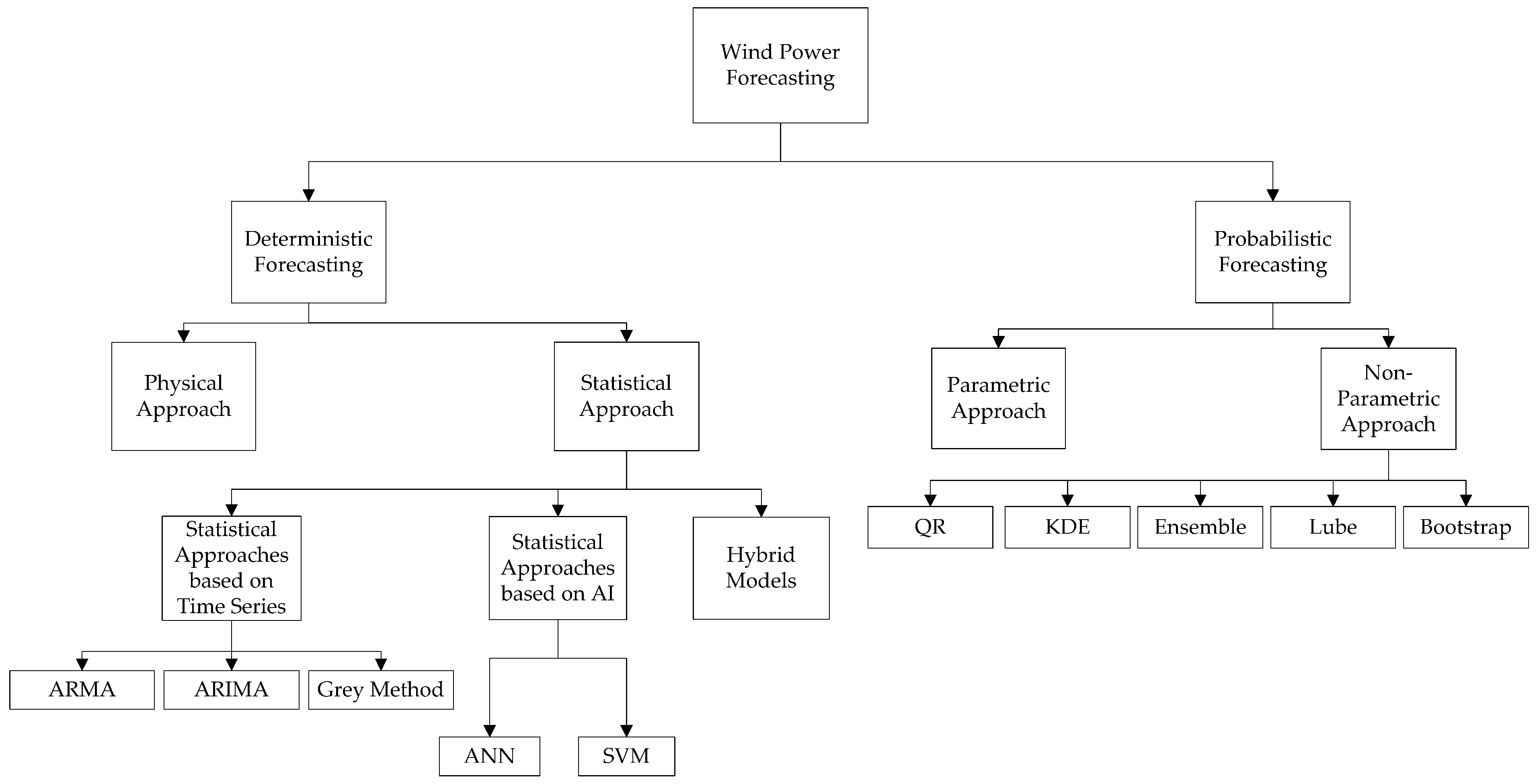
Table 1.
Taxonomy of the statistical approaches used for wind power deterministic forecasting.
| Approach | Reference |
|---|---|
| ARMA | [17,18,19,20,21,22,23] |
| ARIMA | [24,25] |
| Grey Method | [26,27,28] |
| ANN | [29,30,31,32,33] |
| SVM | [34,35,36,37,38,39] |
| Hybrid | [40,41,42,43,44,45,46,47] |
Table 2.
Taxonomy of the approaches used for wind power probabilistic forecasting.
| Approach | Method | Reference |
|---|---|---|
| Parametric | Parametric | [49,50,51,52,53,54] |
| Non-Parametric | QR | [55,56,57,58,59,60] |
| KDE | [61,62,63,64,65,66,67] | |
| Ensemble | [68,69,70,71,72,73,74,75] | |
| LUBE | [76,77,78,79,80,81] | |
| Bootstrap | [82,83,84] |
Table 3.
Contribution of the reviewed works in wind power deterministic forecasting.
| Reference | Published | Contribution |
|---|---|---|
| [34] | May 2004 | SVM was introduced for wind speed forecasting in order to examine its predictive abilities, compared to other NN models. |
| [30] | January 2009 | A comparison between four different ANN models for short-term wind speed forecasting was the main focus. Furthermore, selecting the appropriate parameters for the most suitable ANN model was also investigated. |
| [25] | May 2009 | The suitability of f-ARIMA models towards obtaining more accurate next hour wind speed forecasts is explored, due to their ability to include long range correlations. |
| [31] | November 2009 | An ANN model is proposed for short-term wind power forecasting in order to achieve high accuracy with low computational cost. |
| [29] | July 2010 | Three different types of NNs (FFBP, RBF and ADALINE) were used to investigate the behavior of different NNs while using multiple datasets and evaluation criteria. |
| [32] | October 2010 | A Neuro-fuzzy NN was proposed in order to create a powerful forecasting algorithm that could be integrated in an on-line wind power forecasting system. |
| [43] | December 2010 | Hybrid models based on ARIMA and ANN models were developed to forecast wind speed and wind power with increased accuracy. |
| [35] | March 2011 | An SVM-based model was proposed for short-term wind power forecasting. |
| [40] | April 2011 | A novel, hybrid model based on NN in combination with WT for short-term wind power forecasting was proposed, and its superiority in accuracy and computational cost over conventional forecasting models is shown. |
| [19] | October 2011 | The ARMA model along with the wavelet transform was used to enhance the accuracy of wind speed forecasts in order to reduce the negative effect of wind power to the power grid and supply system. |
| [37] | May 2012 | SVM models along with the wavelet transform were proposed in order to optimize the SVM model and improve its accuracy and computational cost. |
| [41] | June 2012 | The applicability of hybrid forecasting methodology for wind time series was investigated, in order to examine the hybrid models’ superiority over conventional forecasting models for wind speed and wind power forecasting. |
| [24] | July 2012 | An ARIMA-ARCH model was proposed in order to improve the accuracy of the ARMA methodology, taking into account the heteroscedasticity between the fluctuation of wind speed and the characteristics of the change of wind speed. |
| [19] | December 2012 | A comparison between two conventional statistical models, the ARMA model and the ANN, was researched, in order to evaluate their performance and applicability in wind forecasting. |
| [21] | June 2013 | To improve the ARMA model’s accuracy over the time, a combined ARMA-ARCH methodology was used for ultra-short-term forecasting. |
| [22] | November 2013 | The work investigated the efficiency of statistical time-series models in improving the accuracy of short-term forecasts. |
| [38] | February 2014 | A WT-SVM model was proposed and optimized by GA in order to further improve the efficiency and accuracy of the SVM model. |
| [42] | November 2015 | A hybrid EMD-SVM forecasting model was proposed, which improved the accuracy of the forecasts as well as reduced the non-stationary characteristics of the wind data on the predictive results. |
| [39] | January 2020 | A hybrid IDA-SVM model was proposed for short-term wind power forecasting. The systematic analysis with datasets in different seasons showed the increased accuracy of the proposed model. |
| [44] | February 2020 | A BaNN-based hybrid model was proposed for the forecasting process. A filtering and grouping model was also developed based on improved k-means for wind signal prediction. |
| [47] | March 2020 | Different statistical models were proposed and combined for short-term wind power forecasting, including ARIMAX, SVR and MCS power curve models. Via a spatial process, wind speed data from local NWP are adjusted for a specific wind farm and are further used as input for the forecasting process. |
| [46] | June 2020 | A double optimization approach was proposed based on NNs, PSO and GA. Based on these approaches, a WPF model was proposed, using data from a real power plant. |
| [33] | July 2020 | The proposed model used VMD to preprocess and decompose the wind power series. The ConvLSTM was used as the predictor engine in order to remove the noise and extract the spatio-temporal information of the sub-series. |
| [45] | September 2020 | A wind power forecasting model based on WD-LSTM and normalization was proposed to improve the prediction’s accuracy. Furthermore, the normalization and optimization of the input data further improved the predictive accuracy and the model’s convergence speed. |
Table 4.
Contribution of the reviewed works in wind power probabilistic forecasting.
| Reference | Published | Contribution |
|---|---|---|
| [53] | January 2002 | A phenomenological model was tested for the expected distribution of the forecast errors, in order to fully use the output of wind power forecasts. The application of an ANN was used to achieve bias free forecasts with reduced standard deviation. |
| [55] | March 2004 | A LQR model was used to specify the quantiles of the probability distribution of energy production in order to optimize the income function of the producer in energy markets. |
| [57] | December 2005 | Linear quantile regression together with spline bases were proposed to provide quantiles of the forecast error, using only predictable explanatory variables and indices. |
| [59] | March 2008 | A classification of different modeling approaches for probabilistic forecasting was proposed, in order to estimate the most efficient practices for using the available information for accurate on-line uncertainty estimation. |
| [70] | March 2009 | Focus was given to the methodology needed to converse meteorological variables to power generation data. Furthermore, the recalibration of the wind power ensembles to obtain accurate predictive densities was also studied. |
| [71] | March 2010 | Bayesian model averaging, a statistical ensemble postprocessing method that creates calibrated predictive probability density functions, was used to provide calibrated and sharp probabilistic forecasts. |
| [72] | April 2010 | Adaptive resampling approach was proposed in order to provide conditional interval forecasts, in order to successfully complement point forecasts with PIs and to avoid using a pre-assumed shape of the forecast error distribution. |
| [65] | June 2012 | A novel, robust, and time adaptive kernel density forecast algorithm was introduced in wind power forecasting. Apart from being a fully time adaptive model, it also adopted distinct kernels for different types of variables. |
| [51] | August 2012 | A generalized logit-normal distribution was introduced to deal with the non-linearity of wind power generation in wind power forecasting, as an efficient alternative of the conventional normal and beta distributions. |
| [84] | January 2013 | The application of two approaches for construction of PIs for wind farm power generation was proposed, in order to prove their efficiency in giving valid PIs, evading expensive forecasting tools. |
| [54] | March 2013 | The versatile probability distribution model was firstly formulated and its mathematical properties were presented. The model’s accuracy in solving a typical economic dispatch problem was analyzed. |
| [80] | September 2013 | An enhanced version of the nonparametric LUBE method was proposed, using multiple NN models to create PIs and then combining those PIs to obtain more reliable and informative PIs. |
| [81] | November 2013 | A hybrid intelligent algorithm based on interval forecasting approach was developed to produce prediction intervals based on the extreme learning machine and particle swarm optimization, in order to obtain optimal PIs without prior knowledge, statistical inference, or distribution assumption. |
| [83] | November 2013 | A new bootstrap-based ELM probabilistic wind power forecasting approach was proposed, considering the heteroscedasticity of wind power time series. The accuracy and speed of the model was also researched using only historical data. |
| [52] | December 2013 | A methodology was introduced and evaluated that allowed issuing probabilistic wind power forecasts optimally accounting for geographically dispersed information. The main focus was on time-adaptivity in order to reduce the computational cost. |
| [86] | January 2014 | A spatio-temporal analysis framework was proposed that analyzed the dynamics of wind generation by quantifying the statistical distribution and the level crossing rate. Wind power was modeled as a Markov chain and as a result the problem could be studied by Markovian state-space approaches. |
| [77] | February 2014 | A new problem formulation was proposed to create PIs. Furthermore, a new PI width evaluation index, suitable for training NN models, was used. A PSO-based LUBE method was implemented to increase the searching capability of the proposed methodology. |
| [58] | July 2014 | An accurate, efficient, and robust deterministic wind power forecasting model was developed, using a combination of a data filtering approach based on WT and a soft computing model based on FA network. Moreover, SQR was used to evaluate the effectiveness of the proposed deterministic model in a probabilistic sense. |
| [78] | January 2016 | A new fuzzy-based cost function was introduced to satisfy both PICP and PINAW criteria. BA was used for the first time to provide a solution for finding optimal lower and upper bounds of PIs. |
| [88] | March 2016 | An algorithm to determine the contribution of each meteorological station on the next forecasts was proposed. It was proved that combining WT with the proposed spatio-temporal method improved the forecasting model’s accuracy. |
| [73] | February 2017 | CNN was introduced to comprehensively extract the deep invariant structures and hidden high-level nonlinear features of any wind power frequency. A hybrid approach based on WT, CNN, and ensemble technique is proposed for the quantification of the wind power uncertainties. |
| [56] | July 2017 | A novel direct quantile regression approach was proposed for probabilistic forecasting using ELM and QR without prior knowledge, statistical inference, or distribution assumption. |
| [90] | February 2018 | A WPPF model was proposed based on SNN and LUBE, which did not require any prior knowledge or distribution assumption. Furthermore, a new PI optimization model was proposed based on the CPRS. The GSO was also implemented to solve the PI optimization model. |
| [91] | May 2018 | A novel MMC approach was proposed along with a two-step optimization framework. The comprehensive probabilistic combination model was applied for WPF. Evaluation in calibration and sharpness was presented in ten different farms. |
| [79] | December 2018 | The work combined local NWP with wind power generation data to achieve accurate wind power forecasts. Dimension reduction method was used to reduce the computational complexity. A complete hybrid CSS-LUBE model for probabilistic forecasting was developed that could simultaneously process both the historical and NWP data with low computational cost. |
| [87] | April 2019 | A forecasting model based on CNN and PSO was proposed. The wind data was preprocessed with VMD and PSR to give better suited data for CNN. |
| [60] | December 2019 | A joint QR model was proposed for the WPPF, which reduced the effect of the outlying observations and the occurrence of quantile curve crossings. Several conditional quantiles could be directly estimated. The MSSA algorithm was used for the optimization. |
| [94] | January 2020 | An advanced reservoir computing model, TWIESN, was introduced for deterministic and probabilistic WPF. Moreover, a hybrid selection strategy based on RReliefF algorithm and GCRT was selected for the system input. |
| [85] | May 2020 | The EWT method was used to preprocess wind speed time series. Deep NNs were used for the prediction process. The reinforcement learning algorithm was used to integrate three kinds of deep NNs. |
| [89] | July 2020 | A deep mixture density network (MDN) model was designed to provide statistical information in form of PDFs for look-ahead times. A deep network consisting of CNN and GRU was proposed. The reformulation of the MDN could directly construct predictive PDFs, thus gaining in computational cost. |
| [93] | July 2020 | An IDMDN model was proposed for wind power probabilistic forecasting in order to further improve the prediction results of conventional MDN and deep WPF models. |
| [75] | In press | A state-of-the-art methodology on hour-ahead WPPF was developed, that considered the effective preprocessing and postprocessing of the PI. NWP data were combined with measured wind speed data to improve the accuracy of the forecasts. The postprocessing of the PI was implemented to stabilize the forecasting model. |
| [92] | In press | A novel support vector machine model was introduced to improve the learning process of the wind farm active power. Furthermore, a novel FP algorithm was proposed in order to adjust the parameters of the support vectors. |
Table 5.
Comparative results of the deterministic forecasting models.
| Reference | Proposed Model | Compared Models | Parameters of Evaluation | Best Model |
|---|---|---|---|---|
| [20] | ARMA | ANN, Persistence | MAE, RMSE, MRE | ARMA had better performance than both ANN and Persistence |
| [21] | ARMA-Pattern Matching | ARMA | Real data, Relative tolerance | For 0–1 h forecasting horizon single ARMA had higher accuracy. For 1-6hour ARMA-Pattern Matching was better |
| [22] | Various ARMA models | Persistence | RMSE | All ARMA models surpassed the persistence model |
| [24] | ARIMA-ARCH | Single-ARIMA | MRE | ARIMA-ARCH was better with MRE = 11.2% over 17.4% of the single-ARIMA |
| [25] | f-ARIMA | Persistence, Single-ARIMA | DME, σ2, | f-ARIMA was overall better than single-ARIMA. Persistence was better for low wind speed excursions, while for higher ones f-ARIMA and ARIMA gave better results |
| [29] | FFBP, RBF, ADALINE | FFBP, RBF, ADALINE | MAE, MAPE, RMSE | For case 1, based on MAE and RMSE, FFBP was better; based on MAPE, ADALINE had better performance. In case 2, RBF surpassed the other two models. |
| [30] | Various ANN models | ANN1 (3 layers, 3 input, 3 hidden layers, 1output) ANN2(3 layers, 3 input, 2 hidden layers, 1output) ANN3(2 layers, 3 input, 1output) ANN4(2 layers, 2 input, 1output) | MAE, MSE | ANN 4(2 layers, 2 input, 1 output) was the bestmodel with a MAE of 0.0399 and MSE of 0.0016 |
| [31] | ANN | Persistence | MAPE | ANN model was better with a MAPE of 7.26% over 19.05% of the persistence model |
| [37] | WT-SVM | RBF-SVM | MRE, RMSE | WT-SVM outperformed RBF-SVM |
| [38] | WT-SVM-GA | Persistence, SVM-GA | MAE, MAPE | WT-SVM-GA outperformed the SVM-GA and persistence model |
| [35] | SVM | RBF-NN, Persistence | MAE, MAPE, Skill | For both very short-term and short-term forecasting SVM model had the best results |
| [39] | IDA-SVM | DA-SVM, GA-SVM, Grid-SVM, BPNN, GPR | NRMSE, NMAE, MAPE, R2 | The proposed model outperformed all the other models |
| [40] | WT-NN | Persistence, ARIMA, ANN | MAPE | WT-NN outperformed the rest of the models with a MAPE of 6.97% |
| [41] | ARIMA-ANN, ARIMA-SVM | ARIMA, ANN, SVM | MAE, RMSE | Based on MAE, for 1-step forecasting horizon, the ARIMA-ANN had the best results, while for 3-step to 9-step, the ANN and SVM models were better. Based on the RMSE, for 1-step and 7-step forecasting horizon, the best model was ARIMA-ANN, while for the rest, ANN and SVM had the best results |
| [42] | EMD-SVM | SVM | RMS | EMD-SVM had the best results with an RMS value of 15.63% while the SVM had 35.40% |
| [43] | ARIMA-ANN | ARIMA, ANN | ME, MAE, MSE | The ARIMA-ANN surpassed all the other models |
| [45] | WD-LSTM | BMA-EL, MRMLE-AMS, SVR-IDA | MAPE | The proposed model had a significantly improved MAPE value |
| [46] | PSO-PSO-ANN, GA-PSO-ANN | PSO-ANN, Adam-ANN | MSE, MAPE | Both models managed to outperform the PSO-ANN and the Adam-ANN models |
Table 6.
Comparative results of the probabilistic forecasting models.
| Reference | Proposed Model | Compared Models | Parameters of Evaluation | Best Model |
|---|---|---|---|---|
| [55] | LQR Hirlam10, LQR climate | LQR Hirlam10, LQR climate | Sharpness | LQR Hirlam10 had better results from the LQR climate as it gave narrower PIs. |
| [56] | DQR | Persistence, BELM-normal, BELM-Beta, RBFNN | Reliability, Sharpness | Based on reliability, DQR had an APD of less than 2%. As for sharpness, DQR was 25% better than persistence model and 20% better than the RBFNN |
| [58] | Spline-QR-WT-FA-FF-SVM | Spline-QR-BPNN | Reliability, Sharpness, Skill score | Based on reliability, Spline-QR-WT-FA-FF-SVM had lower deviation overall. According to sharpness, the Spline-QR-BPNN gave better results; however based on the final skill score, the proposed model was overall better, especially for a confidence level of 5–35% |
| [59] | SQR, QRF, linear-QR, KDE | SQR, QRF, linear-QR, KDE | Reliability, Sharpness | According to reliability, the QRF and KDE models had close performance, better than the rest of the models. Based on sharpness evaluation, for less than 50% confidence level, all models were equal, but for more than 50%, SQR model had the best results, while linear-QR had the worst |
| [70] | Ensemble forecasts with AKD | Raw ensemble forecasts, ideal values | Reliability, Sharpness | The proposed model showed overall lower deviation and gave narrower PIs |
| [71] | Ensemble forecasts with BMA | Raw ensemble forecasts, Climatology model | CPRS, MAE | The proposed model outperformed the other two based on CPRS and MAE of the point forecasts of the median values of the PIs |
| [72] | 3 pointprediction methods (M1, M2, M3) with adaptive resampling | M1, M2, M3 | Reliability, Sharpness | All three models had a deviation of less than 1.5%. Based on sharpness results, for less than 5 h forecasting horizon, M1 model gave the most accurate results, while for more than 5 h, the M2 model was the most accurate |
| [73] | WT-CNN-Ensemble | Persistence, BR-QR, SVM-QR | ACE, IS, CPRS | The ACE value of the proposed model was improved by 50.84% than the SVM. The IS value was improved by 40.51% than the SVM. As for the CPRS, the proposed method showed the best results in all seasons. |
| [77] | LUBE-PSO | ARIMA, ES, naïve | PICP, PINAW, CWC | Based on CWC, the proposed model had a value of 72.57% while all other models had more than 75%. Furthermore, the LUBE-PSO model had a PINAW value of 72.57% while again the rest of the models were above 75%. As for the PICP, only the ES model, with 92.7% slightly surpassed the proposed model with 91.80% |
| [78] | LUBE-NN-MBA | PSO, BA | PICP, PINAW | In the first study, the proposed method outperformed the other two models. According to the PICP evaluation, the LUBE-NN-MBA had a value of 93.5%, while the BA model had a 90% and the PSO 83.8%. Based on the PINAW evaluation, the LUBE-NN-MBA had a value of 32.96%, while the BA model had a 33.7% and the PSO 38.22% |
| [79] | LUBE-CSS | Persistence | PICP, PINAW, CWC | For a confidence level of 50–90%, the proposed model was better than the persistence model |
| [83] | BELM | Persistence, Climatology, ESM, BELM-Beta | PICP, ACE | According to ACE evaluation, for 95–99% confidence level the value of the proposed model was less than 1%, surpassing the other models. Based on PICP evaluation, for 90−99% confidence level, the BELM model was better than the compared models |
| [84] | MBB-NN | LUBE-NN | PICP, PINAW, CWC | Based on the evaluation metrics, for forecasting horizon of less than 10 min, the MBB model gave better results, while for more than 15 min the LUBE model was more accurate |
Table 7.
Basic features of deterministic models for wind power forecasting.
| Method | Feature |
|---|---|
| Physical | Based on atmospheric conditions; directly connected to the stability of weather conditions |
| ARMA-ARIMA | Can predict future values of a time series through linear regression of the observed values of those time series |
| Grey Method | Powerful tool for forecasting with insufficient data |
| ANN | Evaluation and re-evaluation of input data and their weighed connections |
| SVM | Maps a set of data into high dimensional feature space through a nonlinear mapping process in order to simplify the linear regression process |
| Hybrid | Uses the advantages of combined methods to increase the accuracy of the forecasts |
Table 8.
Basic features of probabilistic models for wind power forecasting.
| Method | Feature |
|---|---|
| Parametric | Assumes a specific distribution shape of the forecasts |
| KDE | Does not assume a specific distribution shape of the forecasts; requires large number of data |
| QR | Gives the uncertainty estimation in the form of predictive quantiles |
| LUBE | Simplifies the PI prediction in one step; low computational cost |
| Bootstrap | Resampling of original data; simplified PI construction |
| Ensemble | Diversity; uses NWP models; gives better results in short and mid-term forecasting |
Publisher’s Note: MDPI stays neutral with regard to jurisdictional claims in published maps and institutional affiliations. |
© 2021 by the authors. Licensee MDPI, Basel, Switzerland. This article is an open access article distributed under the terms and conditions of the Creative Commons Attribution (CC BY) license (http://creativecommons.org/licenses/by/4.0/).
Share and Cite
MDPI and ACS Style
Bazionis, I.K.; Georgilakis, P.S. Review of Deterministic and Probabilistic Wind Power Forecasting: Models, Methods, and Future Research. Electricity 2021, 2, 13-47. https://0-doi-org.brum.beds.ac.uk/10.3390/electricity2010002
AMA Style
Bazionis IK, Georgilakis PS. Review of Deterministic and Probabilistic Wind Power Forecasting: Models, Methods, and Future Research. Electricity. 2021; 2(1):13-47. https://0-doi-org.brum.beds.ac.uk/10.3390/electricity2010002
Chicago/Turabian StyleBazionis, Ioannis K., and Pavlos S. Georgilakis. 2021. "Review of Deterministic and Probabilistic Wind Power Forecasting: Models, Methods, and Future Research" Electricity 2, no. 1: 13-47. https://0-doi-org.brum.beds.ac.uk/10.3390/electricity2010002