Reconstructing the Changes in Sedimentation and Source Provenance in East African Hydropower Reservoirs: A Case Study of Nyumba ya Mungu in Tanzania

Abstract

This study aimed to reconstruct the sedimentation rates over time and identify the changing sources of sediment in a major hydropower reservoir in Tanzania, the Nyumba ya Mungu (NYM). Fallout ²¹⁰Pb measurements were used to estimate age of sediment deposits and broad changes in sedimentation rates were reconstructed. Sedimentation peaks were cross referenced to geochemical profiles of allogenic and autogenic elemental constituents of the sediment column to confirm a causal link. Finally, geochemical fingerprinting of the sediment cores and potential sources were compared using a Bayesian mixing model (MixSIAR) to attribute the dominant riverine and land use sources to the reservoir together with changes through recent decades. Reservoir sedimentation generally increased from 0.1 g cm⁻² yr⁻¹ in the lower sediment column to 1.7 g cm⁻² yr⁻¹ in the most recent deposits. These results correlated to changes in allogenic and autogenic tracers. The model output pointed to one of two major tributaries, the Kikuletwa River with 60.3%, as the dominant source of sediment to the entire reservoir, while the other tributary, Ruvu River, contributed approximately 39.7%. However, downcore unmixing results indicated that the latest increases in sedimentation seem to be mainly driven by an increased contribution from the Ruvu River. Cultivated land (CU) was shown to be the main land use source of riverine sediment, accounting for 38.4% and 44.6% in Kikuletwa and Ruvu rivers respectively. This study explicitly demonstrated that the integration of sediment tracing and dating tools can be used for quantifying the dominant source of sediment infilling in East African hydropower reservoirs. The results underscore the necessity for catchment-wide management plans that target the reduction of both hillslope erosion reduction and the sediment connectivity from hillslope source areas to rivers and reservoirs, which will help to maintain and enhance food, water and energy security in Eastern Africa.

1. Introduction

Hydropower reservoirs support both water and energy security, providing essential services required for development in East Africa [1,2,3]. They are essential for the production of climate neutral energy [4] that guarantees the long-term energy security for economic development in developing countries. Moreover, reservoirs in East Africa provide a source of irrigation and drinking water sources for agriculture purposes and aquatic habits that are beneficial for fisheries and recreation [4,5]. Hydropower reservoirs, however, are increasingly threatened by changing hydrological and sediment dynamics in their wider catchments [6,7]. The driving processes behind the observed increases in sediment delivery in the reservoirs are land use changes, climate change and natural climate variability [8], resulting in accelerating reservoir sedimentation. Subsequently, the water storage capacity is decreasing and energy production capacity also deteriorating [9]. Although dams reduce floods, siltation can cause flooding that may lead to loss of life and property, disruption of the local infrastructure and involuntary resettlement [10,11]. Additionally, siltation of reservoirs can also trigger eutrophication of surface water bodies through release of associated nutrients but also limits sediment transfer to the downstream reaches, thus leading to loss of biodiversity.

The changing demographics of East Africa create increased demand for land, food and water, leading to changes in land and water use [10,11,12]. These land use changes increase the vulnerability of soils to the impacts of hydroclimatic drivers of erosion by water [13]. An increased rate of soil erosion is one of the main drivers of land degradation in East Africa’s agropastoral landscapes [14], which often severe impacts on community resilience and socioeconomic development [15,16]. Furthermore, changes in precipitation under global climate change also alter the dynamics of river flow and discharge [17,18]. While some exploratory work has been performed on the potential impacts of climate change and land use in East African hydropower reservoirs [3,19,20,21,22] and the estimations of the sedimentation rate [19,23,24], there is little quantitative evidence available on the changing sedimentation rates and sediment sources contributing to the infilling of reservoirs. In this context, some pressing questions remain regarding hydropower management now and in the future. What are the major potential sources of sediments contributing to the infilling of the reservoir? What are the best techniques to assess reservoir sedimentation rates? What approaches can reduce the quantity of sediment incoming to the reservoirs from upstream? How might future climate change affect sediment supply? Radiometric dating using fallout radionuclides (FRNs) and geochemical fingerprinting (sediment tracing technique) can fill in this caveat in empirical data. These empirical models can subsequently be coupled with information on changing land use and climate to make meaningful deductions on the driving processes of increased sediment delivery. The present study therefore will reconstruct the sedimentation rate over time in the Nyumba ya Mungu reservoir (NYM) using fallout radionuclide (FRN)-based nuclear techniques (¹³⁷Cs and ²¹⁰Pb dating techniques) and quantify the main riverine and land use sources to the sediment using geochemical fingerprinting.

Reconstructing changes in rates of reservoir sedimentation since dam closure is crucial for evaluating the extent of siltation problems and therefore the durability of hydropower reservoirs. Sediment tracing techniques evaluate the similarities and dissimilarities between the physical or chemical traits of downstream sediments and the catchment potential sediment sources [25,26,27]. Consequently the geochemical composition of downstream reservoir sediments depends on the relative contributions and geochemical properties of different tributaries [28,29,30]. The proportional attribution of the tributary sources to downstream sediment can therefore be obtained through integration of the multivariate source and mixture geochemical fingerprints within mixing models [30,31,32,33]. This is, however, only possible when the eroded soils of the fine particle fraction (e.g., particle size < 63 μm) transported from different watershed areas behaves conservatively from detachment, transport, deposition and after deposition.

The FRNs, ²¹⁰Pb and ¹³⁷Cs, can be employed to study erosional records of a catchment via dating of downstream sediment accumulation (e.g., in a reservoir) and, therefore, the effects of land use and climate by presenting data from different time windows during the last 100–150 years [34]. The fundamental ability of ²¹⁰Pb_ex to provide evidence on the chronology of a sediment deposit and thus estimate the sedimentation rate depends on its source in relation to local geology, its moderately long half-life, and its retrospective assessment that provides a longer-term (ca. 100 year) chronology or age–depth relationship [35]. The anthropogenic radionuclide, ¹³⁷Cs, is from weapon testing fallout that peaked in early 1960s. However, its fallout in tropical Africa was low, challenging its application [36]; ²¹⁰Pb is a natural geogenic radionuclide—its deposition is continuous and basically constant from year-to-year [36]. Generally, the rate of decrease of ²¹⁰Pb_ex activity with depth in a sediment core offers the foundation for developing an age–depth correlation and for estimating sediment accumulation rates (SAR) [37]. From its activity profile, it is feasible to determine the sedimentation rate and in some conditions to reconstruct environmental changes [36] through time using numerous models comprising a variety of assumptions [36,38,39,40].

2. Materials and Methods

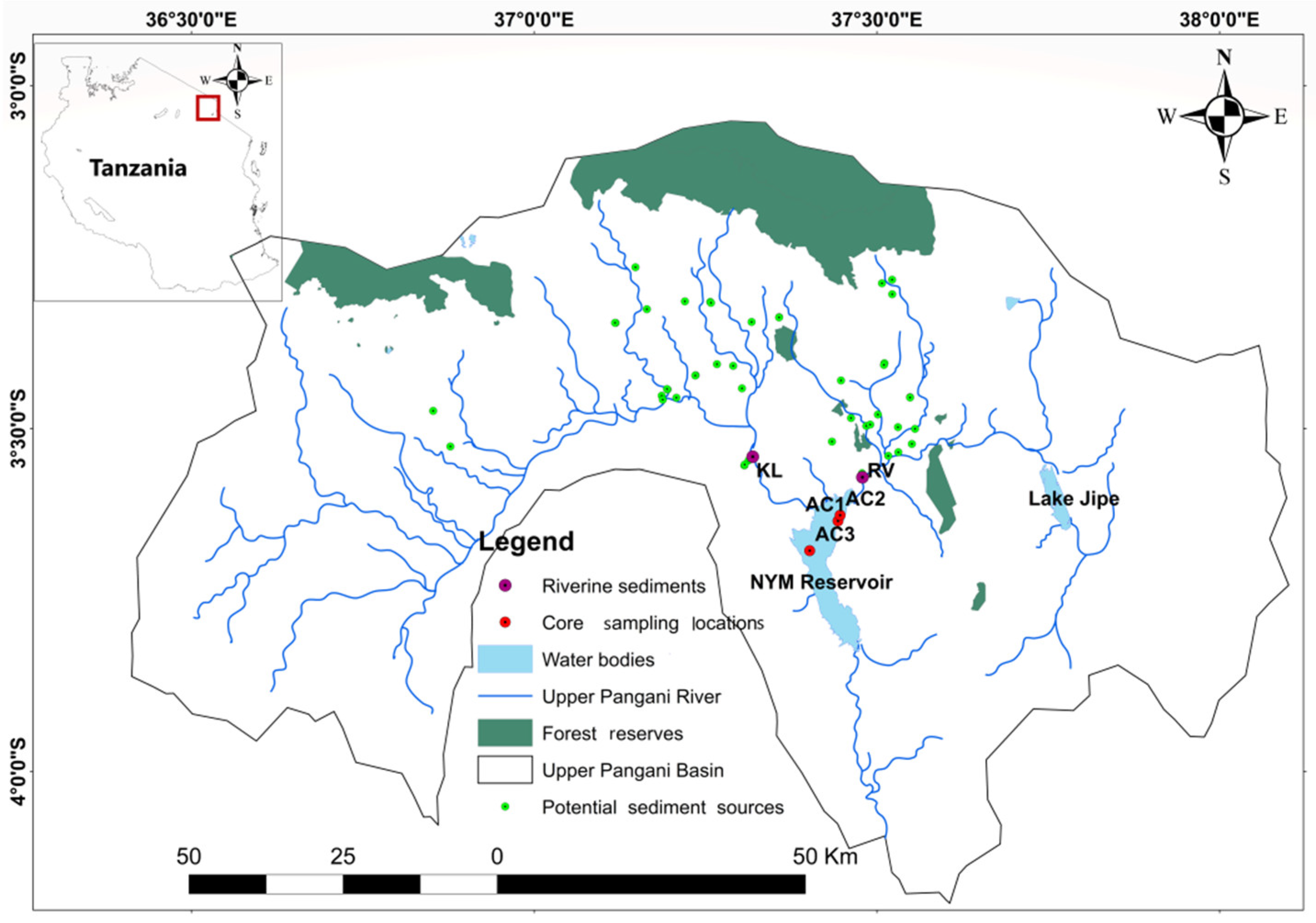
2.1. Description of the Study Area

NYM is a constructed reservoir that largely replaced a natural wetland when the river was impounded. The NYM catchment includes the highlands of Africa’s highest peak, Mt. Kilimanjaro (5985 m), and fifth highest peak, Mt. Meru (4566 m). The reservoir is part of the upper Pangani River Basin (PRB) and receives water from two main tributaries, the Kikuletwa and the Ruvu rivers (Figure 1). The Kikuletwa subcatchment covers about 6650 km² out of 12,000 km² and the Ruvu approximately 5350 km² of the total catchment. The dam was erected in 1965 for hydropower generation but in later years, irrigation potential was realized and integrated into strategies [23,41,42]. The NYM reservoir is about 150 km², has a live-storage capacity of about 875 million m³ [43] and has a maximum depth of 40 m [44,45]. However, due to highly variable climate and changing sedimentation, these factors fluctuate seasonally and between years.

The catchment of the NYM reservoir is located between latitudes 3°00′00″ and 4°3′50″ south, and longitudes 36°20′00″ and 38°00′00″ east, and its altitude ranges between 700 and 5825 m.a.s.l. The ice cap at the peak of Mount Kilimanjaro forms the highest ground in the catchment. The catchment occupies a total land and water area of about 13,000 km² [46] and experiences a tropical climate that provides high levels of precipitation with average annual rainfall (AAR) of 900–2200 mm/year at 800 m.a.s.l and 2200 m.a.s.l, respectively [44,45,47,48], (Appendix A). The catchment experiences bimodal rainfall, occurring mainly in March to May with short rains in November and December [49,50]. The temperature gradient of the catchment is closely related to altitude, ranging from 15 to 33 °C, with the maximum and minimum temperatures occurring during February and July, respectively [48] (Appendix B). The catchment land cover types change in response to the changing elevation, ranging from montane forests on the higher altitudes to semiarid in the lower slopes. The major land cover types include natural forests, woodlands, grassland thickets with emergent trees, bushland and plantation forests [51]. The geology upstream of the dam is characterized by volcanic rocks composed of the olivine and alkaline basalts, phonolites, trachytes, nephelinites and pyroclastics [43,48,52]. The majority of the population settlements are located on the lower slopes between 900 and 1800 m.a.s.l, where most agricultural activities are concentrated. The ever increasing demand for food with an increasing population in the NYM catchment within the Pangani River Basin, Northern Tanzania, has led to rapid expansion of agricultural land, thus accelerating soil loss rates and downstream siltation of the reservoir [30,53,54,55,56,57].

2.2. Sampling Strategy

Three 28 to 32 cm cores were taken from the reservoir, two close to the mouth of the adjacent river input and one more distant (Figure 2). The core locations were limited by logistics and chosen so that they included a temporal record of sediment deposited in the reservoir. Frequent flooding to the villages nearest the headwaters of the reservoir was an indication of the high siltation in the inlets. Shallow depth in the middle of the lake and presence of mostly coarse (sand to gravel) sediments in some locations in the middle was the reason for the abandonment in sampling in the middle of the reservoir. In addition, due to the presence of hippopotamus, certain areas in the lake were also avoided. To this end, efforts were mostly concentrated close to the inlets to account for spatially specific and localized sedimentation effects. Water depths of the core locations spanned between 1.6 and 3.0 m (site AC1 = 1.8 m; AC2 =1.6 m; AC3 = 3.0 m). A corer, fixed inside with PVC tubes (60 cm length and 8 cm in diameter) was manually pushed into the sediment by divers. The cores were kept in upright positions in the boat for some hours where their overlying waters were gently decanted. The PVC tubes were consequently opened from one end, after which each core was subsectioned at 2 cm intervals to obtain a sufficient temporal resolution, while keeping a high analytical accuracy [58]. The core sections were stored in polyethylene bags and transported to the laboratory where they were weighed wet and then oven-dried at 50 °C to constant weight, in order to determine dry bulk density. The dried sliced cores were subsequently disaggregated using a mortar and pestle and then sieved.

The tributary riverbed sediment samples (DS) were collected from lower reaches of the two major tributaries, Kikuletwa (KL) and Ruvu (RV), assuming that the transported and deposited sediments offer a representative sample of the composite mixture from their respective sources in the entire catchment. Fourteen and eighteen samples of the respective tributaries were collected over a range length of about 200 m to include potential spatial differences in riverine sediment deposition [30,59,60]. DS sample collection depended on the environmental and logistical constraints in the system. Due to the ephemeral nature of the rivers, DS samples were generally collected in the dry season from the exposed beds. Land use soil samples were recovered from agricultural topsoil (CU), bushland topsoil (BS), channel banks (CB) and mainstem river banks (RB). The agricultural and bushland topsoils involved surface soil (0–5 cm) sampled from areas presumed vulnerable to water erosion and their connectivity to river network. Sampling of subsurface/channel bank material was done in upstream areas characterized by exposed banks devoid of vegetation with actively eroding bank sections due to flow incision by high water energy released during heavy rainfall. Eroding mainstem river banks were also sampled. Sampling locations for the land use samples depended on the accessibility, necessary permits and safety. At each site, samples comprised a composite of 10 to 15 random scoops pooled into a single composite sample to ensure the representativeness of the corresponding fingerprint property datasets. A total of 57 samples were collected to characterize four main potential sediment sources: (i) bushland (BS, n = 15), (ii) channel banks (CB, n = 15), (iii) cultivated agricultural land (CU, n = 14) and (iv) mainstem river banks (RB, n = 15), all collected in one-year season. Soil and tributary sediments were also oven-dried at 55–60 °C to constant weight and consequently disintegrated using a mortar and pestle and then sieved.

2.3. Radiometric and Geochemical Laboratory Analysis

Radiometric analysis and the geochemical analysis of the cores in loose powder form were done at the Consolidated Radioisotope Facility (CoRiF) Laboratory of the University of Plymouth certified under ISO9001:2018, while the geochemical analysis of the potential sediment sources in pressed pellets was done at the Tanzania Atomic Energy Commission (TAEC).

2.3.1. Radiometric Analysis

The sliced sections of the sediment cores were filled into aluminum canisters and sealed for a minimum of 21 days to account for the secular equilibrium between ²²⁶Ra and its progenies. The activity concentrations of the radionuclides in the subsequent section cores were analyzed using low-background EG&G Ortec planar (GMX50–83-LB-C-SMN-S) and well (GWL-170-15-S) HPGe gamma spectrometers. Sediment cores were counted for 24 h, analyzing the gamma spectra of the natural radionuclides ²¹⁰Pb (46.5 keV), ²²⁶Ra (via ²¹⁴Pb and ²¹⁴Bi peaks at 352 and 609 keV, respectively) and for the anthropogenic radionuclide ¹³⁷Cs (662 keV). The samples with low masses were counted for 48 h, and their results were cited with a 2σ counting error. Excess ²¹⁰Pb (²¹⁰Pb_ex) activity was determined as the difference between total ²¹⁰Pb and supported ²¹⁰Pb (in equilibrium with the parent radionuclide ²²⁶Ra). A natural homogenized soil, with low background activity and spiked with a radioactive traceable standard solution (80717-669 supplied by Eckert & Ziegler Analytics, Atlanta, GA, USA), was used to perform the calibration of the gamma spectrometer. GammaVision software was used to establish the geometry-specific calibration relationships. Analytical performance was assessed by participation in IAEA worldwide proficiency using example soils (IAEA-CU-2009-03 and soil IAEA-TEL-2012-03).

2.3.2. Geochemical Analysis

Before analysis, all dried samples were homogenized and sieved to <63 μm fraction to minimize particle size effects on tracer signals that can bias fingerprint property [13,32,61,62]. The elemental concentrations are generally enriched in the fine, < 63 μm, particle size fraction in comparison to <2 mm bulk fraction of the soil [13,63,64]. For comprehensive reviews on issues of particle size effects on sediment fingerprinting, readers are referred to [61]. Subsequently, about 4 g of dried and sieved sample material was mixed with about 0.9 g of cellulose binder (FLUXANA^®), homogenized in a pulverizer and pressed into a pellet of approximately 32 mm diameter. The method was validated by using the IAEA Soil 7 certified reference materials (CRM) described in [65].

The core samples were analyzed for minor and major elemental geochemistry by wave length dispersive X-ray fluorescence (WD-XRF; PANalytical Axios Max; OMNIAN application) as loose powder. The sediment certified reference material was used to validate the analyses (GBW07318, LGC, Middlesex, UK). The dried soil and tributary potential sediment sources were analyzed by an energy dispersive X-ray fluorescence (EDXRF) spectrometer coupled with Xlab ProTM software as pressed pellets. For assessment of the analytical variability and sample homogeneity, triplicates were made from arbitrarily selected samples about once every 3 samples. Only those elements returning measurements above the limit of detection (DL) were employed in the analysis (DL varies with the element and depends upon several factors including the sample matrix). The difference in the analytical methods for the major and minor elements may have influenced the accuracy of the model.

2.4. Data Analysis

2.4.1. Sediment Chronology and Mass Accumulation Rates

The rate of change in ²¹⁰Pb activity with mass depth in a sediment core provides the basis for an age–depth relationship and for estimating sediment mass accumulation rates (MARs) [30,41,66,67]. The comparatively long half-life of ²¹⁰Pb (t_1/2 = 22.23 years) provides the basis for the age determination processes of up to 5–6 half-lives, i.e., ~100 years. For the purpose of reconstructing variations in sedimentation rates over time, the constant rate of supply (CRS) model was used because it assumes a constant ²¹⁰Pb flux but allows the sediment supply to vary [38] (Appendix C). This model was successfully applied in a nearby complex catchment that had experienced catchment-wide environmental changes [30]. However, a major limitation of this technique in complex East African catchments is that a significant fraction of ²¹⁰Pbex supply to the sediment deposits may originate from older catchment material [68]. In large catchments there might be natural variability in the terrestrial geological prevalence of ²³⁸U that can influence the ²¹⁰Pbex activity from the secondary ²¹⁰Pbex activity. In addition, the natural variability might be caused by the dissimilarity in prevalent erosion processes [69] that can change the fraction of topsoil vs. subsoil in the transported sediment material, affecting the ²¹⁰Pbex activity [30,36,70,71]. Consequently, whether the atmospheric ²¹⁰Pbex flux to the reservoir environment acts steadily stable over time, the arriving secondary ²¹⁰Pbex fingerprints from deposited sediment might differ significantly [68]. Owing to potential differences in ²¹⁰Pbex fluxes, the CRS model outcomes were scrutinized through comparison with another independent marker, ¹³⁷Cs (t_1/2 = 30.17 years), from its 1965 peak fallout [72] in the southern hemisphere using the fitting approach (CRS-fitted) as described in Appleby [34] (Appendix D). However, due to the low levels of ¹³⁷Cs fallout in tropical Africa and the known date of dam construction, the deepest sediment layers were also fitted to the reference date of 1969 using the fitting approach (CRS-fitted) as described in Appleby [34] and in Appendix C and Appendix D. Finally, the geochemical profiles of the cores were also scanned for distinct changes or peaks that could be linked to hydrological or sedimentological changes [30,73].

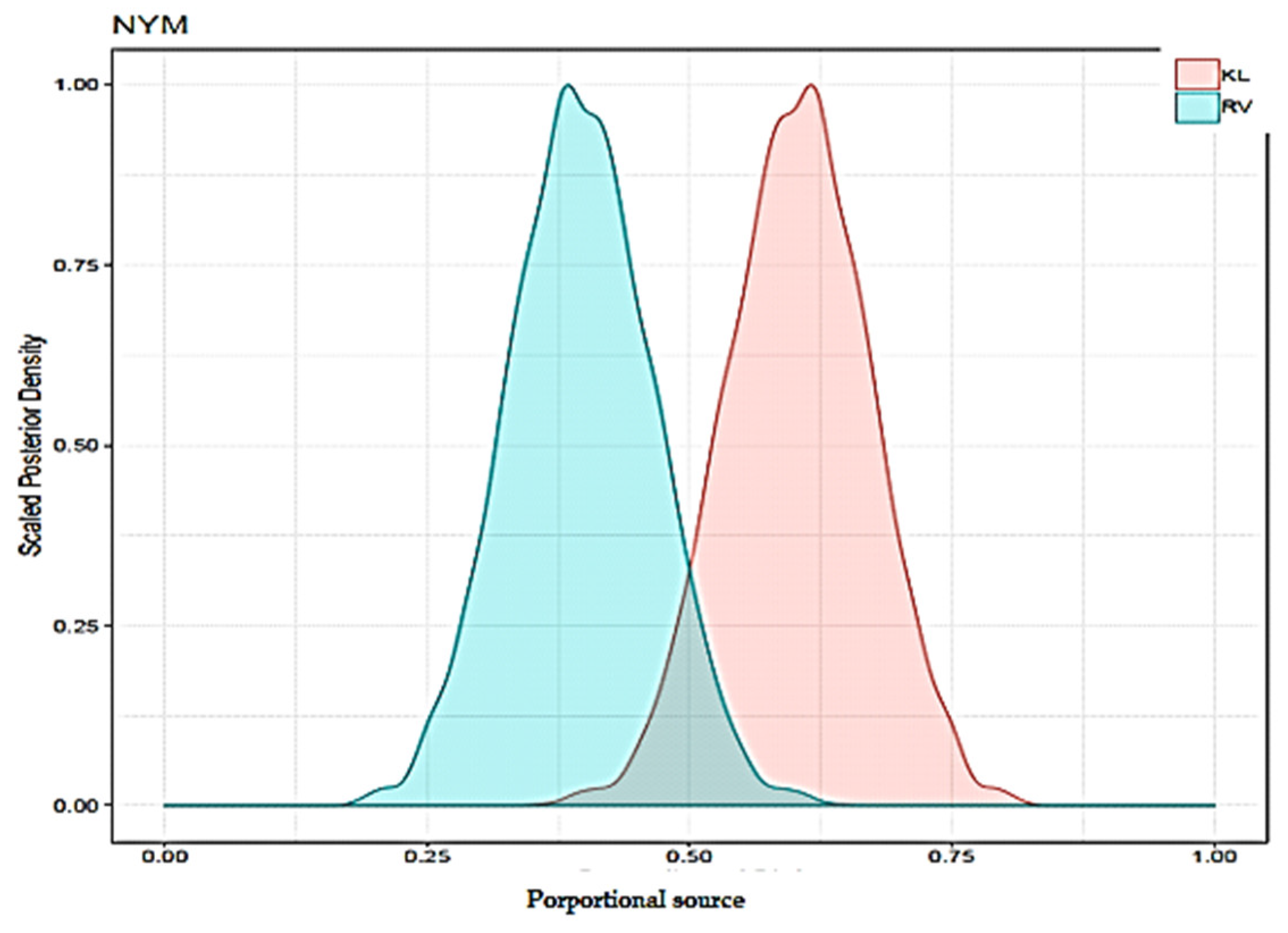
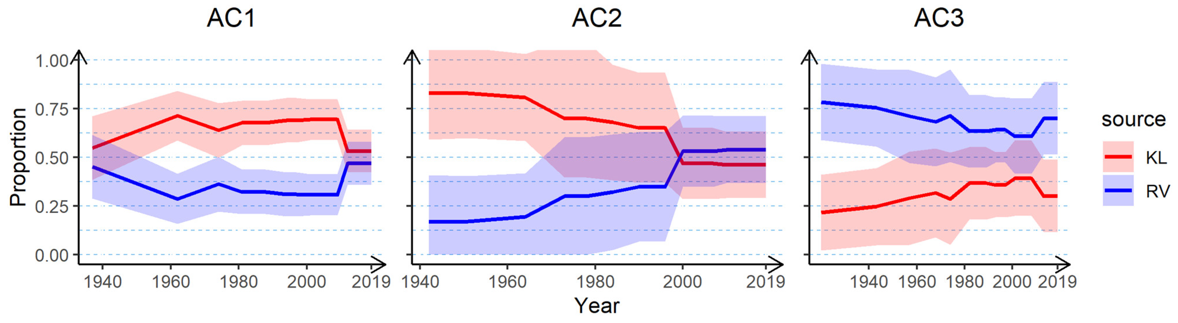
2.4.2. Bayesian Mixing Model (BMM) for Source Apportionment

After the broad spectrum geochemical analysis, each sample can be represented as a multielemental concentration data point. The fingerprints of the potential sediment sources and the lake mixture form multivariate concentration matrices on which the model is drawn to quantitatively compare different sources with the lake mixture. A Bayesian mixing model was built in the open-source MixSIAR framework [74,75,76], as first demonstrated by Blake et al. [31] for river basin sediment source apportionment. For comprehensive details of the mathematical formulation of MixSIAR, readers are referred to Stock et al. [74]. The deconvolutional MixSIAR (D-MixSIAR) methodology was used to hierarchically unmix the tributary sediment against the core sediments and subsequently unmix the land use source fingerprints against the tributary sediment. For the BMM to accurately represent the system, it depends on the following four assumptions: (1) the model includes all dominant sources contributing to the sediment, (2) the value of the tracers are known in both sources and mixture, (3) tracers behave conservatively throughout the mixing processes and (4) fingerprint variability between sources is larger than within sources.

Tracer Conservation Test

In order to make a direct comparison of the properties of the sediment samples with those of the potential source materials, tracers need to behave independently and conservatively (assumption 3) in the environment [31,77]. This implies that the chemical composition of the tracers does not alter during detachment, transport or after deposition [61,78,79].

The source apportionment results were achieved using a tracer selection procedure that only excluded tracers on the basis of nonconservative behavior from literature evidence of potential mobility in aquatic systems [80]. Initially, all elemental concentrations from the depositional samples that fell outside the minimum detection limits were removed. Thereafter, the basic tracer screening approach of Blake et al. [31] and Sherriff et al. [81] was adopted with additional evaluation of geochemical behavior. For each set of sources and associated mixtures for all tracers, boxplots were produced and the means of the mixture data assessed to see if they largely fell within or outside of the mean concentrations of the different sources [31] (Appendix E). Tracers wherein the mixture fell outside the source range were removed. In addition, the tracers that were found to be higher in intrasource variance than the intersource variance were also removed. Finally, the normality assessment using the Shapiro–Wilk test for the individual tracer mixtures was done because the model assumes normal distribution of the mixture tracer data [74]. Seven tracers passed the range test (P, Ti, Mn, Fe, Zn, Sr, Nb) and 7 borderline tracers (S, Co, Ni, Cu, Ga, Ba, Hf) were also retained and engaged. Model efficacy was evaluated using the Gelman–Rubin diagnostics [82]. Seventeen tracers (Na, Mg, Al, Si, Cl, K, Ca, Cr, Br, Rb, Zr, Ce, Pb, Th, La, Y, Sn) were eliminated from the analysis based on the evidence of nonconservative behavior or high intrasource variability. These exclusions warrant some geochemical clarification. Sr and Rb may have been caused by their known variability in the soil depth as a function of weathering processes and mixing of soil horizons by cultivation [83]. Nonconservative behavior of Mg, Na, Ca, Cl, F, K and Br can be explained by their tendency to form highly soluble salts [31] driven by evaporation in the lake [84]. La, Ce and Th were removed because of the observed intersource variability, which are potentially an artifact of analytical challenges due to low abundance or high variability in the terrestrial source concentrations [30]. Various elements, such as Al, are known to exhibit nonconservative behavior during fluvial transport and short-term storage in river channels [85], while other tracers (Si Cr, Y, Pb and Zr) are known to undergo transformations in medium- to long-term storage elements such as floodplains, lakes and wetlands due to changes in redox, pH, salinity and other environmental conditions [86,87,88]. Concentrations of Al, Si and Zr may be due to wider fluvial sorting, e.g., textural controls on mineral composition, i.e., changing proportions of silt versus clay minerals in mixtures, which has been shown to exert a strong influence on sediment concentrations [89]. The older sediment deposits, however, may have undergone diagenetic processes within the sediment column [90].

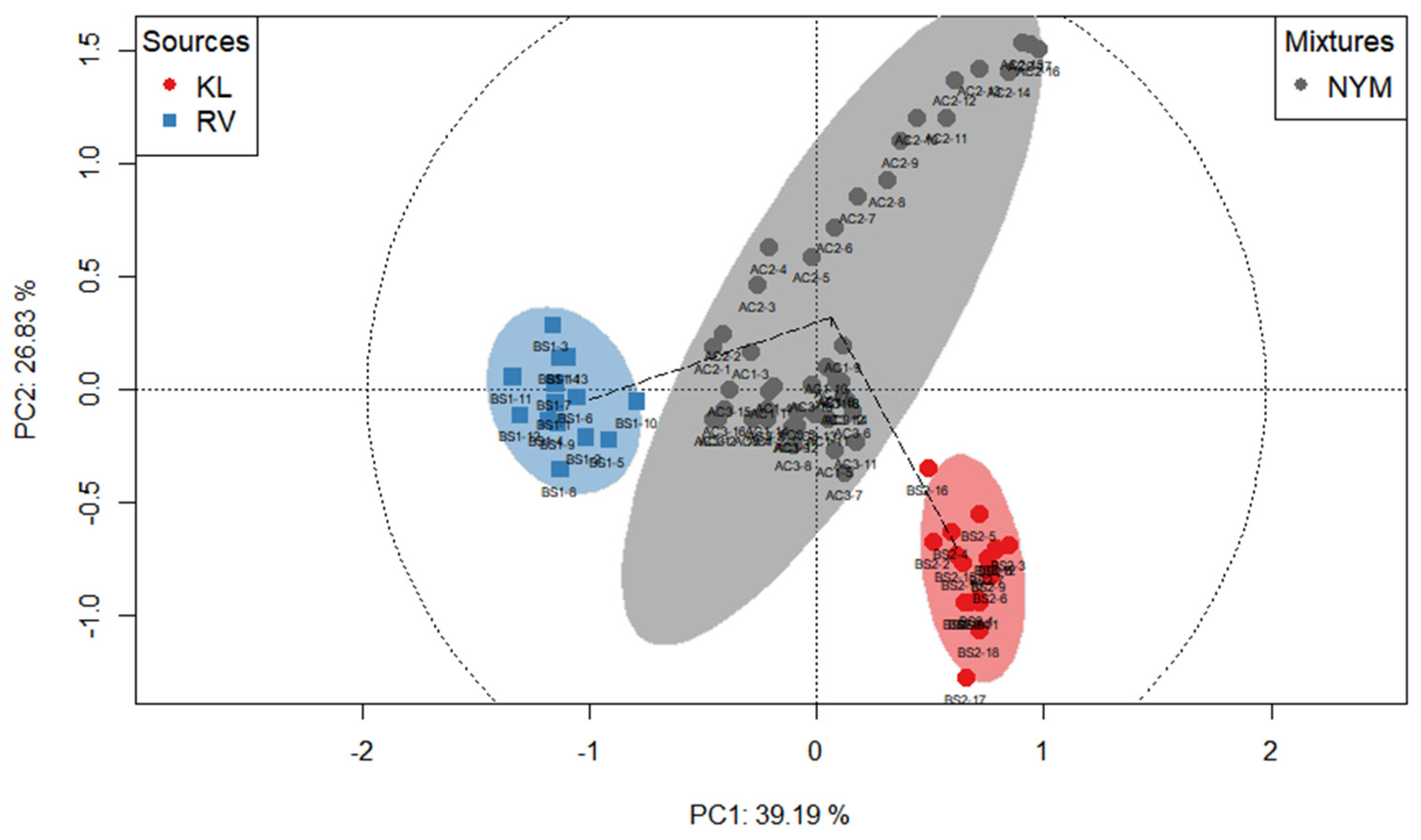
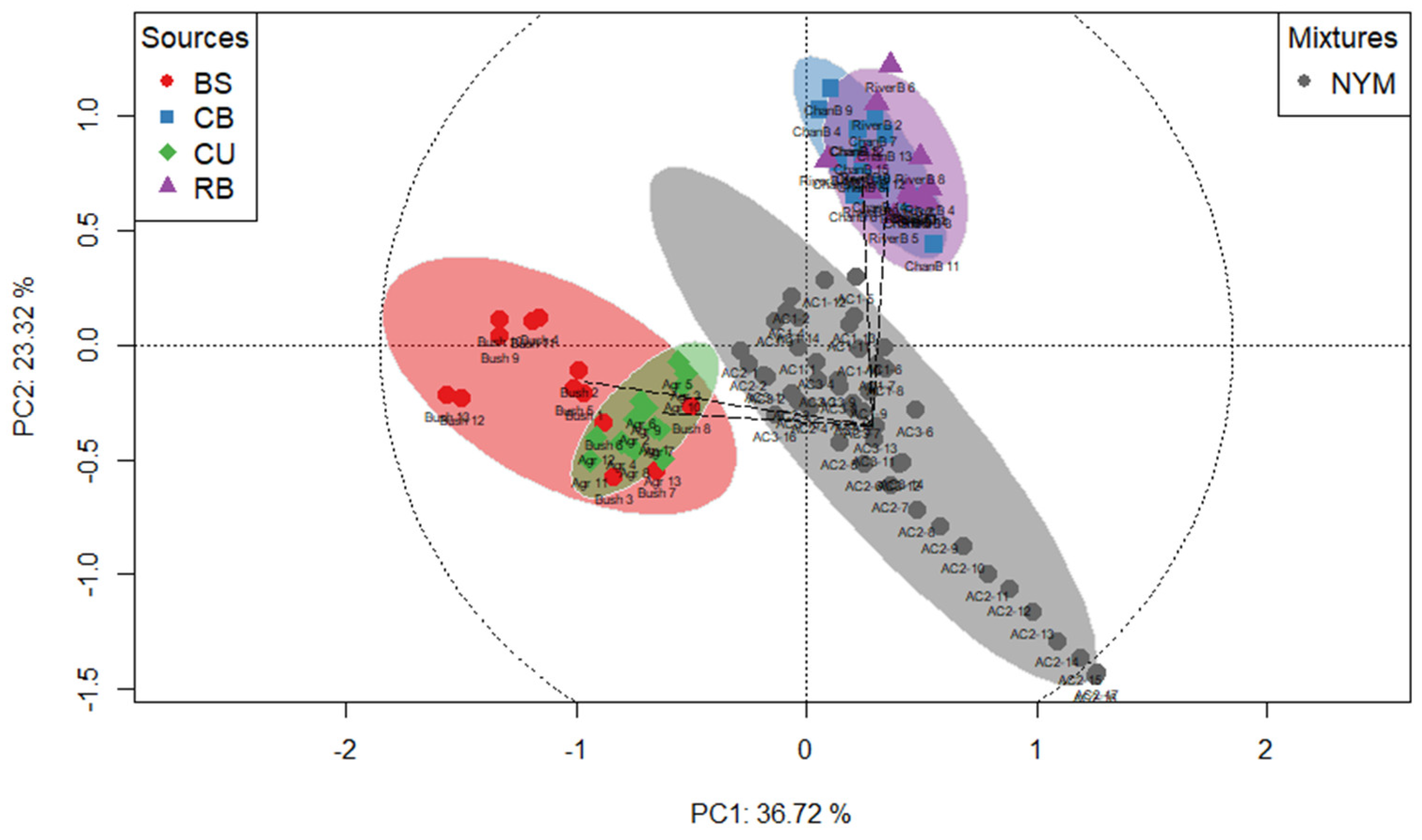
Principal Component Analysis (PCA)

PCA was performed to accommodate assumption 4, which requires the intersource differences of fingerprints to be larger than the intrasource differences in fingerprints. It is in this context that the PCA was performed to analyze variance in multitracer datasets and reduce dimensionality [90] from the potential sediment sources data into land use specific and tributary categories according to their geochemical composition.

Model Build and Running Protocols

(1) Error formulation: Eroded soils with distinct geochemical properties form the wider catchment mix from the source to a mixture through mixing process. However, in these complex systems it is impossible to capture the total variability in sediment source sample by sampling. Therefore, a “residual error” formulation was integrated in the model. Since the transport of sediment from channel networks to the reservoir is random and constant, a “process error” was not included [74,75].

(2) Since there are no other sources of empirical information concerning the sediment source contributions to the reservoir, an uninformative prior was used: (1, 1, 1, 1) and (1, 1) for land use and tributary sources, respectively.

(3) A mixture of sediment samples was analyzed without fixed or random effects to infer the proportions of the tributaries and land uses to the “total” reservoir sediment. Afterward, a fixed categorical effect of the sediment mixture from reservoir sampling locations was established to infer the proportions of different land uses and tributaries to the specific sampling location in the reservoir. The ascription of sediment delivery over time was inspected by using individual sediment cores whereby the “age” was introduced as a fixed continuous effect. Subsequently, the sediment core slice samples were grouped into distinct classes whereby the depth was established as fixed categorical effect. The model outputs were assessed under different modes of covariate structure.

For all model runs, the following stipulations were used: a residual error term only and an uninformative Dirichlet prior (α = 1). Model convergence was assessed by the Gelman–Rubin diagnostic (variables < 1.05), rejecting model output if >5% of total variables were above 1.05. Model convergence indicates that the model found a singular solution to the problem. The MIXSIAR model using the selected 14 tracer fingerprints on the sediment sources passed the Gelman–Rubin convergence diagnostic with the parameters of the Markov chain Monte Carlo (MCMC) chain run length set as follows: chain length = 1,000,000, burn = 700,000, thin = 300, chains = 3.

3. Results and Discussion

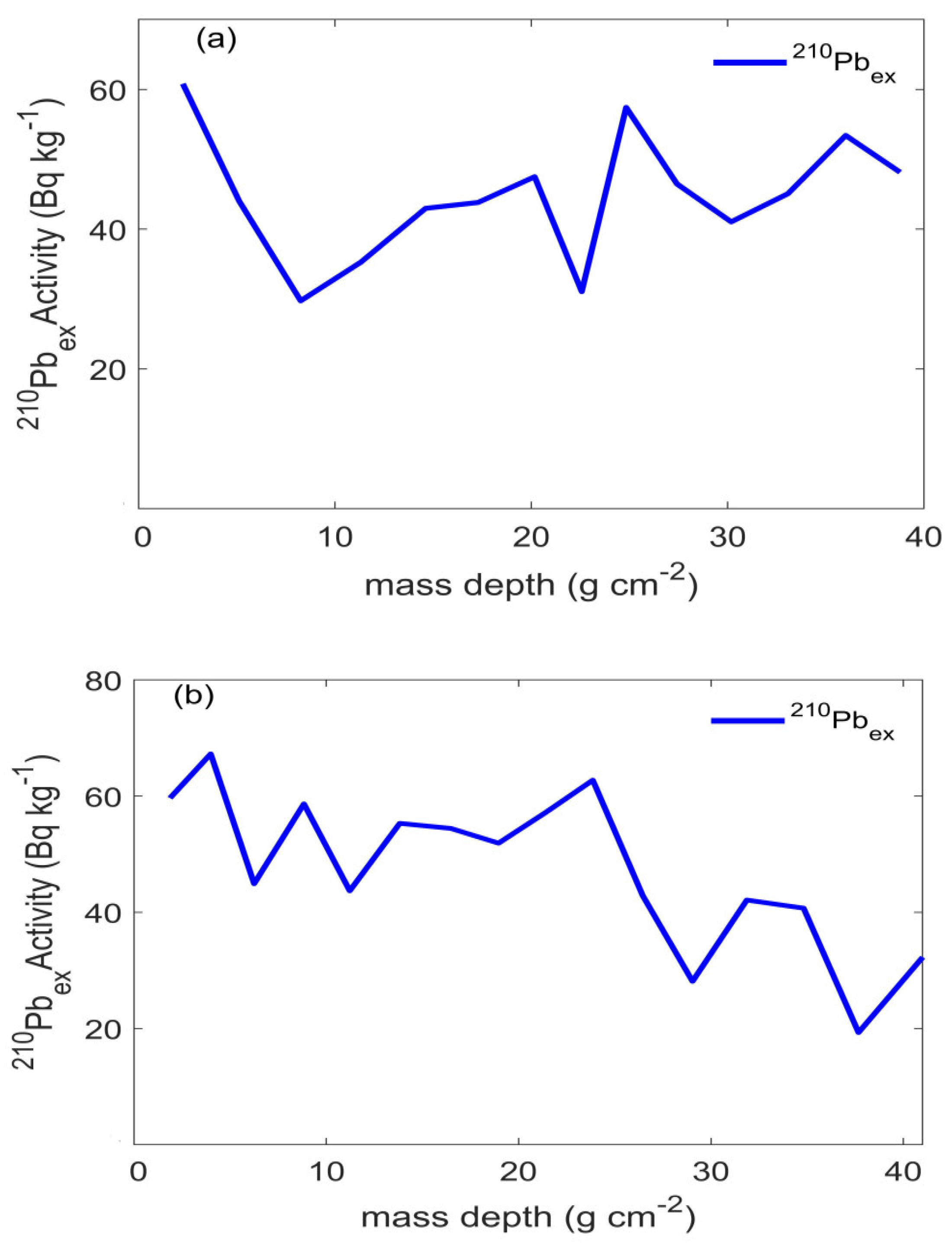
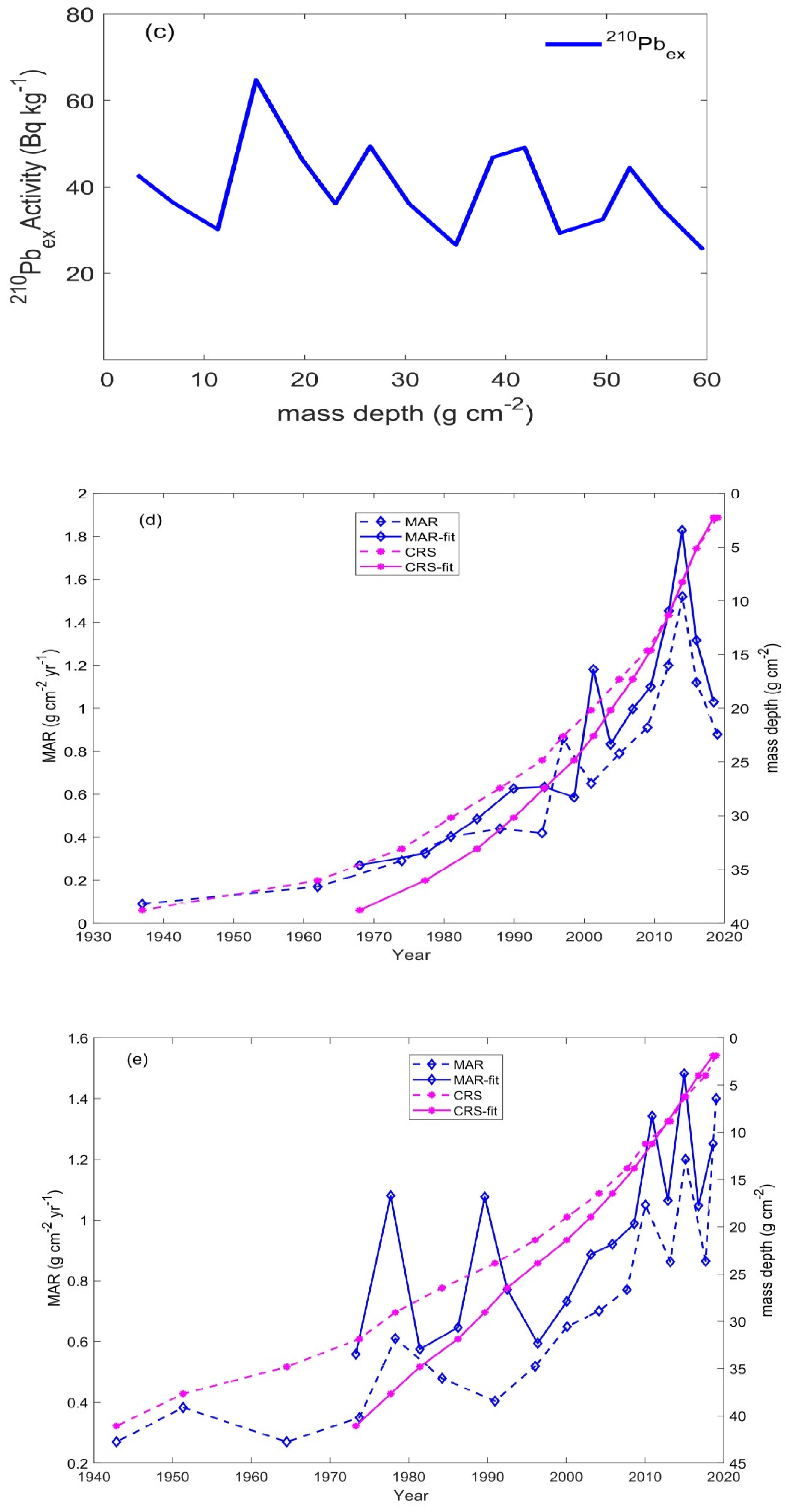
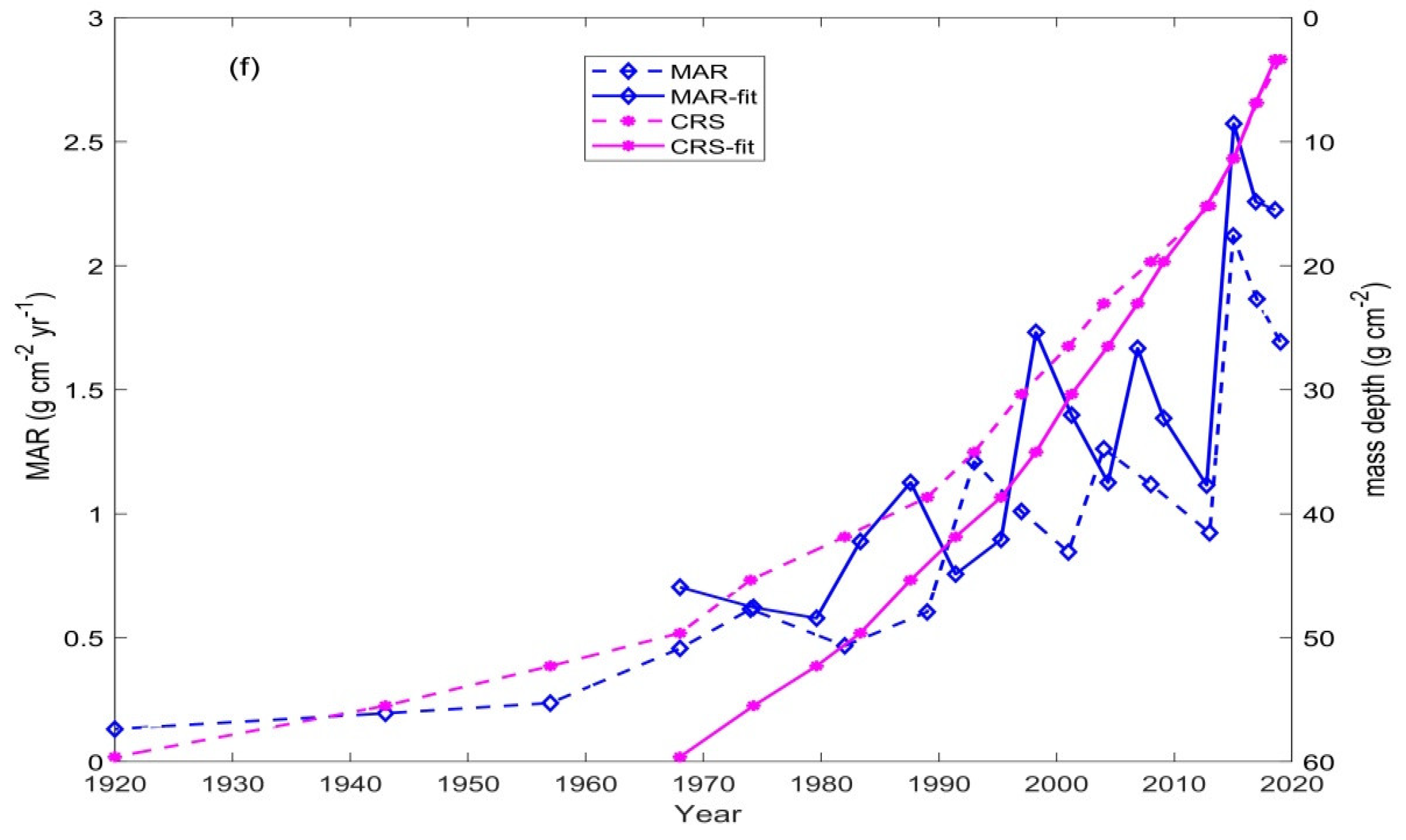
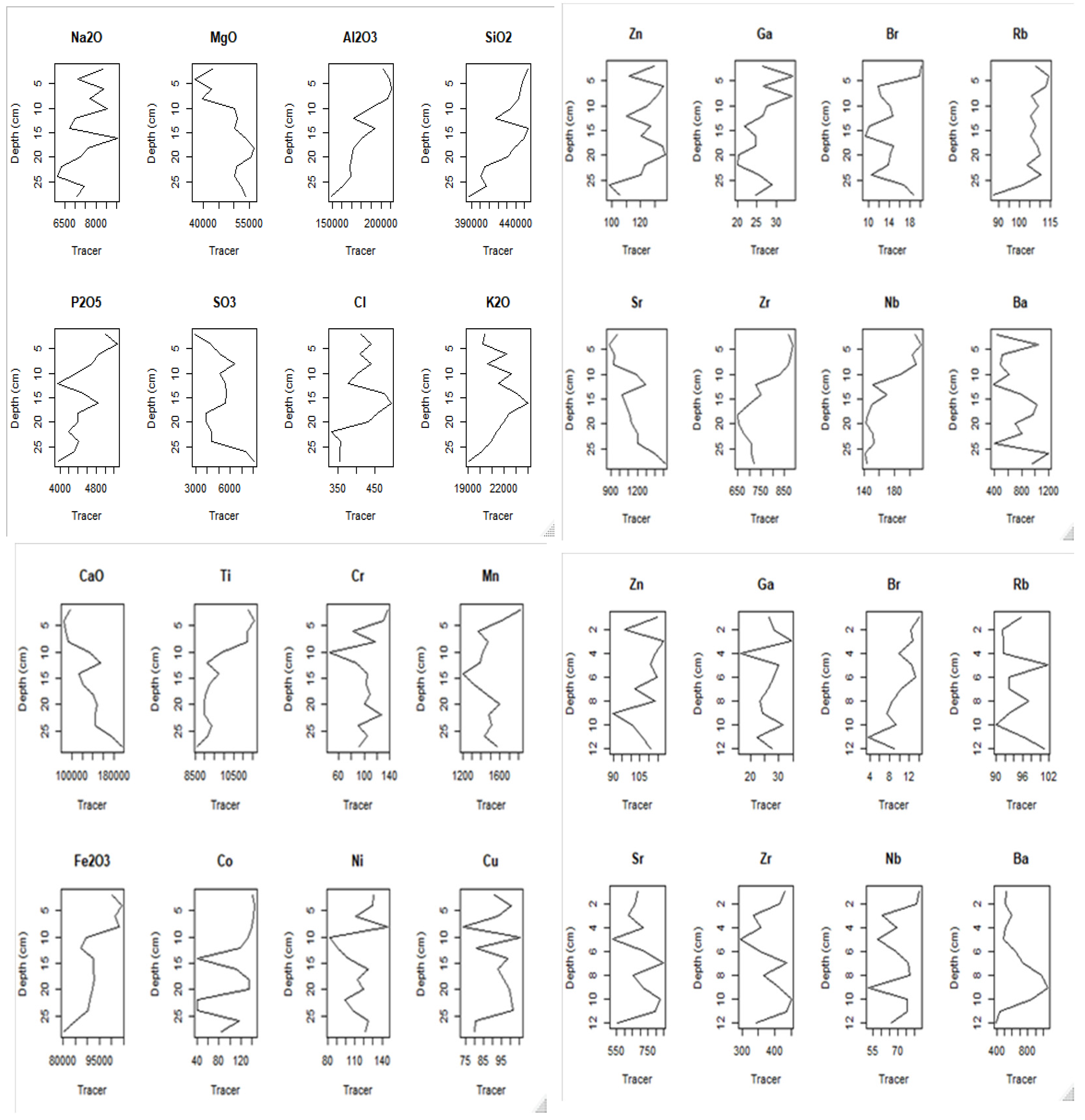
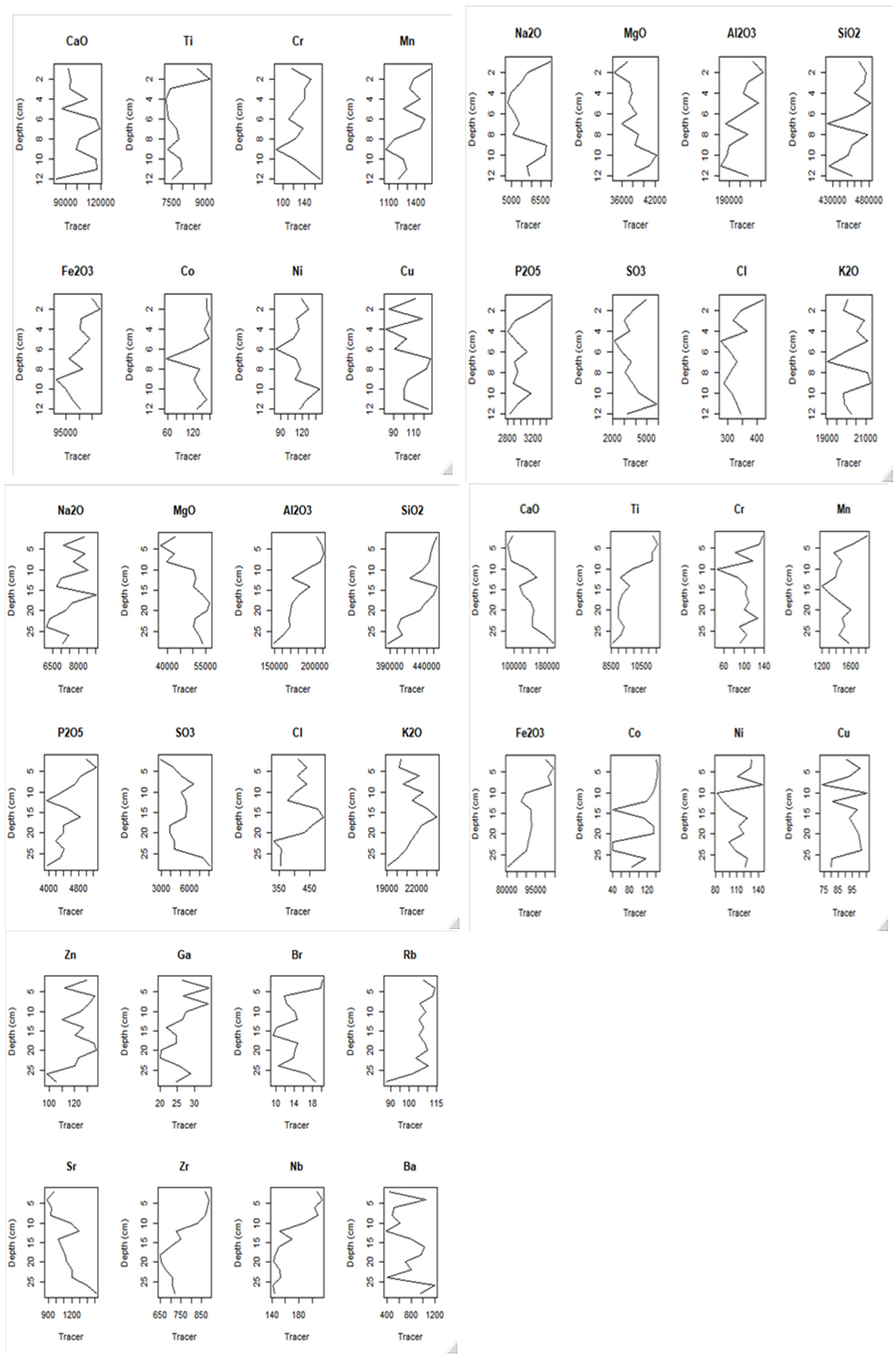
3.1. ²¹⁰Pb_ex and ¹³⁷Cs Vertical Profiles

The ²¹⁰Pb_ex profiles (Figure 3a–c) of all three cores did not follow an exponential decline with depth and were instead characterized by multiple peaks and troughs indicating episodic increase in sedimentation rate, which would have diluted the ²¹⁰Pb_ex activities of the more recently deposited sediments [30,34]. However, a number of processes could have also resulted in the vertical mixing in the sediment cores. First, high energy water flows and wave action at the river inlets could have led to vertical mixing of the sediment deposits and a flattening of the ²¹⁰Pb_ex. Second, human and biological activities might also have led to mixing of the upper sediment layers in the shallow parts of the reservoir. Third is the variation in the remineralization of sediment particles downcore. Furthermore, previously discussed variations in the direct atmospheric depositional flux of ²¹⁰Pb due to fluctuations in the annual amount of rainfall and variation in the secondary input of the ²¹⁰Pb from the catchment could have influenced the ²¹⁰Pb_ex profile [68].

The ¹³⁷Cs activity concentration, where detected, was low in all of the cores, with most of the sections below the limit of detection. These results are similar to the global ¹³⁷Cs fallout estimates in tropical regions [35]. The low ¹³⁷Cs activities obstructed the assessment of ¹³⁷Cs peak integrity and the comparison of ²¹⁰Pb radiometric dates with independent ¹³⁷Cs peaks [3]. Contrary to core AC2 and AC3, core AC1 had a significant single measure of ¹³⁷Cs activity above the detection limit (Appendix F). The detectable layer was assumed to be the 1965 southern hemisphere peak deposition [35,91]; however, the ”peak” might also be related to secondary transport of catchment surface material to the reservoir, meaning that it could be younger than 1965 [68,92]. For these reasons, the ¹³⁷Cs dating and fitting the CRS models of the NYM reservoir cores using the ¹³⁷Cs dates would result in a high level of uncertainty. Therefore, two versions of the CRS model were run. The first “standard” approach estimated dates based solely on fallout ²¹⁰Pb_ex. In a second “fitted” model, it was opted to fit the deepest sediment layers to the construction date of the dam. In the former case, the assumption is that the core penetrates the post impoundment soft sediment into the original substrate. In the latter, there is an assumption that the coring captured the full soft sediment profile.

Under CRS standard approach model version, the observed changes in sedimentation dynamics could be associated with the construction of the dam, but also by higher levels of soil erosion following deforestation and agricultural degradation. The changes in 1970s correspond with the adoption of the “villagization policy” in Tanzania, which led to practicing of a cooperative economy (communal production) through collective farming [93,94,95]. The sharp MAR peaks 0.86 and 1.01 g cm⁻² yr⁻¹ in the mid 1990s in cores AC1 and AC3, respectively, may be linked to ENSO, specifically, the 1997/1998 El Niño events [96] (Figure 3d,f). These general trends of sedimentation dynamics in cores AC1, AC2 and AC3 in the 2000s to 2010s is related to growing urbanization, extension of agricultural activities and the loss of permanent vegetation through the rapid expansion of agricultural land [12,22,96,97,98].

The alternative CRS-fitted geochronology model approach of Appleby [34], using 1969 as a fixed date, showed a similar trend of changing sedimentation dynamics as the CRS-standard approach. While the MAR of cores AC1, AC2 and AC3 and age–depth relationship using the standard CRS approach were found to be relatively similar (Figure 3d–f), the MAR-fitted trends were also found to be similar between the different cores. There were some interesting differences observed between the CRS-standard and CRS-fitted approaches in each individual core. For instance, the MAR-fitted trends in core AC3 were higher than those in core AC1 and core AC2. Due to the smaller time range, the MAR-fitted rates and peaks were much higher, giving rise to a more punctuated profile. However, the general observed trend of increasing sedimentation over time was observed in both approaches. While extreme rainfall during the ENSO 1997/1998 El Niño events [95] seems to have contributed to higher rates of sedimentation in the NYM reservoir, this was not observed for the higher rainfall in 1978/79 (Appendix A). Under this model scenario, this seems to confirm that the increase in sedimentation in the NYM reservoir was driven by a complex interaction between natural rainfall variability and increasing vulnerability to soil erosion through land use change. The differences observed in the timing and heights of the MAR peaks between the cores might be due to spatial differences in sedimentation due to the dynamics of sediment transport from the dominant riverine sources, as will be further explored in Section 3.3. Difference in particle settling velocity due to different locations of the cores might be another reason for the variations in sedimentation rates. However, the main limitation of the CRS-fitted approach fitting the curve to 1969 is that it might have included the activities from the floodplain of the natural wetland before the date the reservoir was commissioned in 1969.

The geochemical profiles of the sediment cores offer a useful indication of changes in tributary sediment delivery to NYM reservoir over time to help constrain and interpret the different geochronological models. Comparing the broad trends of the CRS output of all model versions with their geochemical profiles allowed for catchment-based contextualization of the modeled MARs [30]. The recent MAR peaks in all cores closely matched with peaks in many elements connected to allogenic sediment origins and minima in elements linked to evaporative autogenic tracers, as shown in Appendix G [84]. The allogenic tracers Fe, Ti, Zr and Nb, Rb, Ba and Ga and the evaporative autogenic tracers Mg, K, Na, Ca and Sr have corresponding maxima and minima at the same depth (4 cm) in 2016 and 2017 for cores AC1 and AC3, respectively, as the MAR peak. However, in core AC2, the allogenic tracers Al, Ti, Ni, Cr and Fe and the autogenic tracers Na, S, Cl, Sr and Ca have distinct maxima and minima at 2 cm in 2019 and 5 cm in 2016, respectively, while the evaporative autogenic tracers Mg and Na have the minima corresponding to maxima of the allogenic tracers. This high correlation between geochemical tracers of allogenic sediment delivery and reconstructed sedimentation peaks in both cores reciprocally validates both evidence bases, making it highly likely that NYM reservoir recently experienced extreme sedimentation rates driven by increased erosion and sediment transport from the catchment. The difference in concentrations was observed between the cores; the variation in geochemical concentration is not only caused by changes in absolute sediment delivery, it may be attributed by the difference in source contribution (e.g., from different tributaries) and erosion process (e.g., subsurface vs. surface) which also cause changes in profile. The difference in concentration can also be due to location-specific sedimentation effects (e.g., more or less sedimentation and/or higher contribution from one of the tributaries). Interestingly, the difference in concentrations was also observed between the deepest older sections and upper recent sections of the autogenic (Na, S, Cl, Sr, Ca) and the allogenic (Al, Ti, Ni, Cr, Fe) tracers. The concentrations of the autogenic tracers were much higher in the deepest sections and lower in the upper recent sections and vice versa for the allogenic tracers. The possible reason is that the deepest core sections are from before reservoir construction, i.e., “standard” geochronology model, or the older sediment deposits may have undergone diagenetic processes within the sediment column [90].

An additional consideration to the limitations of ascribing exact dates to the sediment column is that the²¹⁰Pb_ex profiles are vulnerable to sediment reworking through biological and physical activities such as bioturbation and fishing [99]. Following these occasional events, the ²¹⁰Pb_ex profiles are interspersed and might be difficult to determine [100]; however, in many cases, an indication of broad rates of SAR change can still be determined with notable evidence for changes in sediment provenance being a key observation [37].

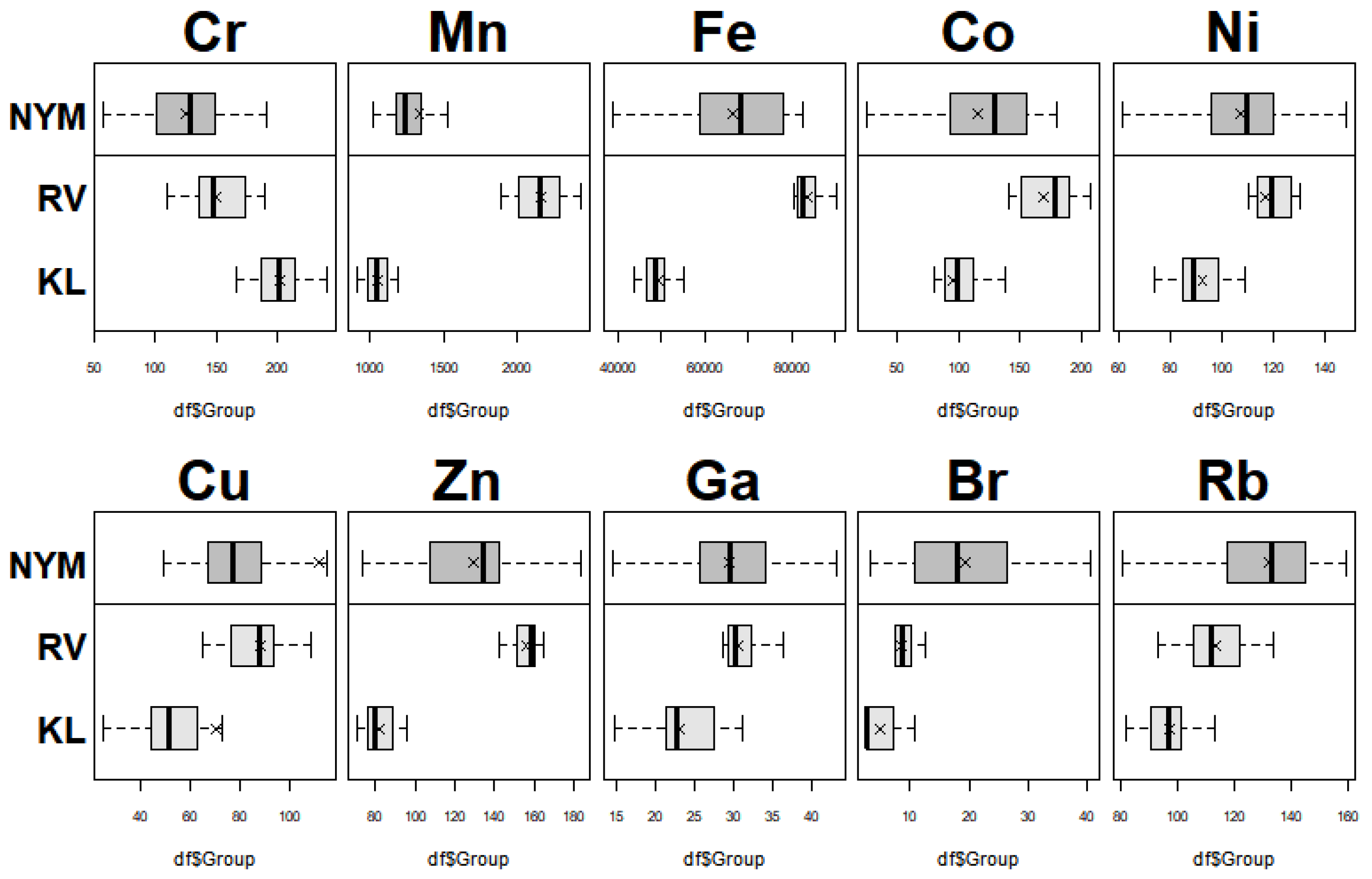
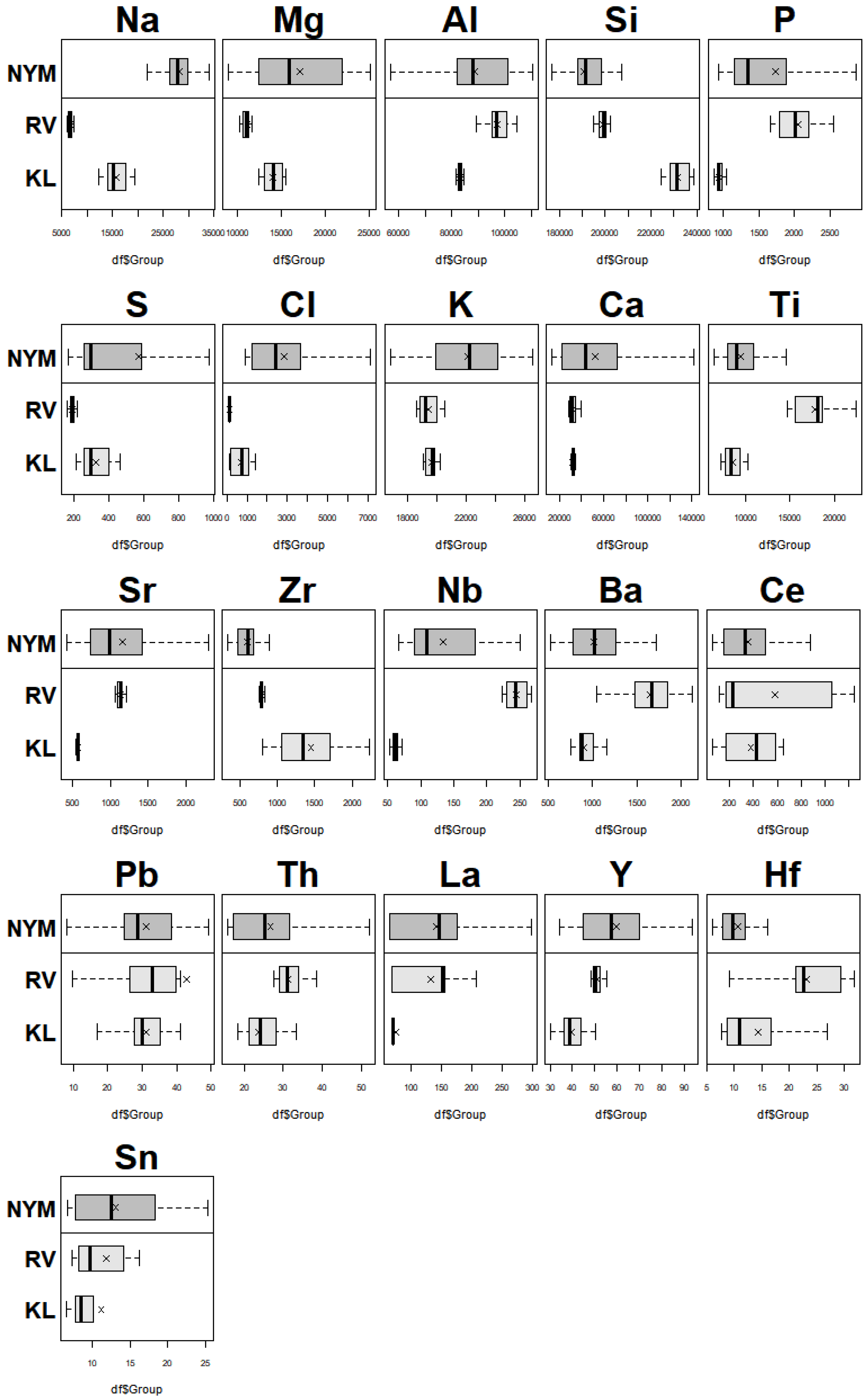
3.2. PCA for Statistical Analysis of Data

The temporal and spatial distinctiveness of the source fingerprints identified show distinct fingerprint clusters between the two tributaries (Figure 4) and a low level of overlap between the land use sources, the RB and CB, while CU and BS show distinct fingerprints (Figure 5). The reduced discrimination between the RB and CB may be due to source signatures to resemble a mix of RB and CB, given both are subsurface materials and presumably less weathered. Overall, however, the signatures provide a clear basis for sediment attribution [101,102].

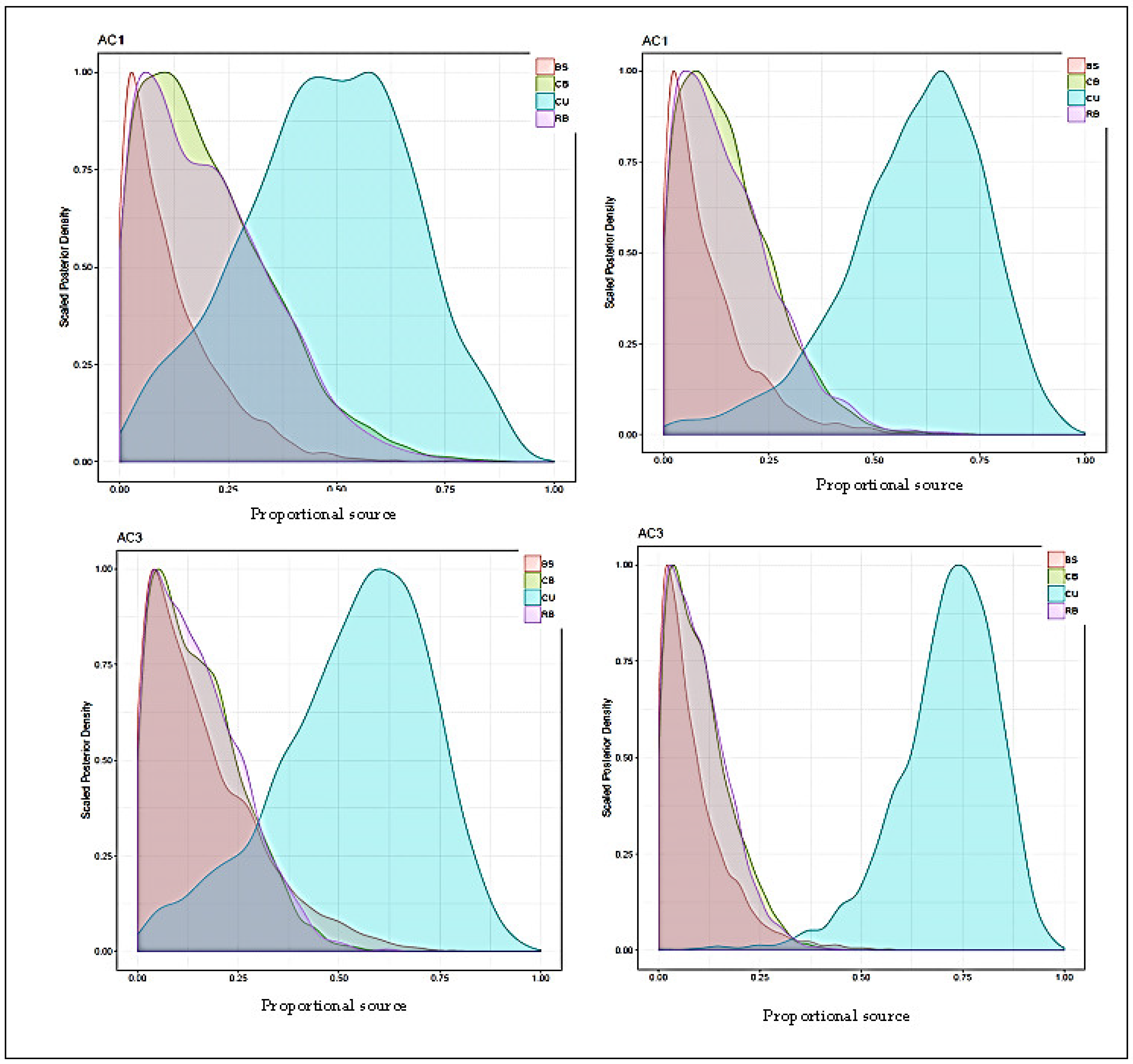
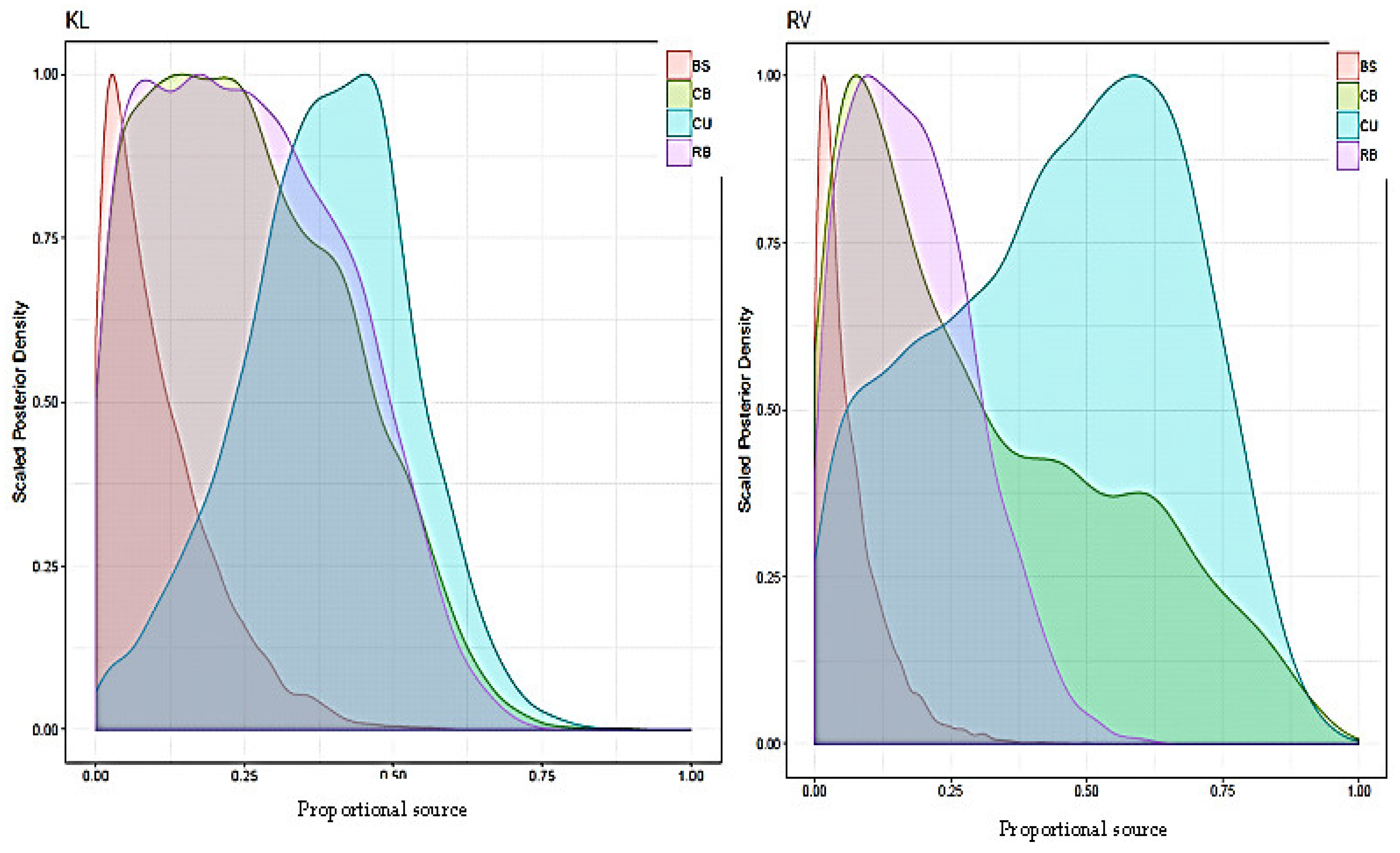
3.3. Proportional Tributary and Land Use Contribution

The BMM outputs revealed that the Kikuletwa River contributed 60.3% of ”total” reservoir sediment and the Ruvu River 39.7% (Figure 6). While the Kikuletwa River is the dominant contributing tributary to the total reservoir sediment, cores AC2 and AC3 have a higher proportional contribution of Ruvu sediment with 55.4% and 51.8%, respectively (Appendix H). The dominance of Ruvu in AC3 is counterintuitive since the location of AC3 is farther from the Ruvu inlet. However, sedimentation dynamics are also regulated by other factors besides distance to the inlet, such as the dominant flow direction and velocity at the river inlets. Overall, the contribution seems to be well balanced between both rivers.

The sign of changes in tributary sediment delivery to the NYM reservoir over time is evidenced by the geochemical stratigraphic record of the sediment cores that experienced distinct periods of high and low sedimentation associated with changes in tributary sediment delivery (Figure 7). Unmixing the core sections over time yielded changing proportional contributions of the river systems. The proportional contribution of KL in core AC1 seemed to have increased in the lower core before reverting back to almost 50%. RV decreased from the lower to mid core and then remained stable over time before a slight increase in the upper core. In core AC2, the proportion of KL showed a continuous decrease from 83.1% in the lower core to approximately 50% in the upper, and vice versa for RV. Core AC3 also shows an increase of KL over time, after experiencing a distinct drop in contribution in the upper core (Appendix H). Integration of the changing proportional contribution and reconstructed MAR seems to indicate that the most recent increase in sedimentation is mostly driven by increased sediment delivery from the RV system. This finding seems to indicate that increased erosion and sediment transport from the RV system are driven by increased land use change in the catchment. This result corresponds with previous research by Mzuza et al. [43] using magnetic properties showing that RV is the most recent contributing tributary. This association of land use change was also observed using the older and the recent core sections of AC1 and AC3, respectively (Appendix H). The comparison was made following the trend of increasing sedimentation rate in core AC1 and AC3 (Figure 4e,f) with the relative source contribution (Appendix H) and (Figure 8).

Unmixing of the core sections directly against the land use pattern demonstrated a significant increase of sediment contribution from the agricultural land (CU) and decrease of the BS, CB and RB in older and younger sections of cores AC1 and AC3. CU increased from 47.6% (lower core) to 59.6% (upper core) while BS, CB and RB decreased from 11.6%, 20.5%, and 20.3% to 10.1%, 15.4% and 14.9%, respectively, in core AC1 (Appendix H) and (Figure 8). A similar trend was observed in core AC3 where CU increased from 53.5% to 71.0% while BS, CB and RB decreased from 16.1%, 15.1% and 15.3% to 8.7%, 10.3% and 10.0%, respectively (Appendix H) and (Figure 8). The increase in contribution from CU corresponds to the previous studies that observed high levels of deforestation and the loss of permanent vegetation through the rapid expansion of agricultural land and growing urbanization [12,22,96,97,98]. The decrease in the contribution of the BS, CB and RB is proportional to the increase in CU and the increase in sedimentation in younger core sections, increasing the evidence for changing dynamics of soil erosion and sediment deposition in the reservoir during recent years.

Unmixing of the land use types against the riverine sediment revealed that the Kikuletwa tributary had a greatest contribution of sediments from CU (38.4%), and the other types also had significant contribution, RB with 25.6%, CB with 25.5% and BS with 10.5% (Figure 9, left, and Appendix H). The CU on Ruvu River accounted for 44.6% of the sediment contribution, CB with 31.0%, RB with 18.0% and BS with 6.4% (Figure 9, right, and Appendix H). These findings corroborate with previous research showing that both subcatchment have high soil erosion risk due to unsustainable farming practices [12,22,47,96,97,98]. The farming practices in both subcatchments may have increased the sediment connectivity to the channel networks due to less buffering of the soil [103]. Although most of the irrigated large-scale plantations are located on the lowlands, sediment sources might have originated from the sloped small-scale agricultural plots and not from the lowland irrigation agriculture. In addition, the use of floodplains for agriculture might have increased the sediment routing to the lake. The evidence of eroding river and channel banks as important sediment sources in fluvial systems [104,105,106,107] is underscored by the concentration of the geochemical tracers in the Ruvu River (Appendix H). The steady increase in the concentration of the Mn, Sr and S [85,108,109] with depth supports the hypothesis of the channel banks and gully erosion. The anthropogenic land use changes or natural alteration of geomorphology dynamics of channel and river bank dimension in the watershed may have influenced the subsurface erosion of the allogenic sediment delivery to the reservoir. In addition, the changes in the catchment land cover types from montane forests on mountain slopes to semiarid grasslands [12] in response to climate change impacts [15] and land use pressures [17,18] may have increased the hillslope erosion, thus increasing the structural sediment connectivity to the channel networks.

Overall, the fingerprinting analysis shows that cultivated land was the dominant source of the riverine and total reservoir sediment. However, these results should be inferred as estimates and not complete observations because of the temporally and spatially constrained representations of geochemical fingerprints, the geochronological model assumptions and structure and tracer selection protocols. Nevertheless, the compatibility of model output proves the general strength of the methods and the significance of sediment input from this system.

A major challenge of the approach used here is that the riverine sediment fingerprint originates from samples spanning one year, while the cores integrate >60 years. The riverine sediment thus does not include potential variations in sediment fingerprint over time. However, given the strong difference in signature between the Kikuletwa and Ruvu river sediment, it is assumed that intrasource variations will remain smaller than intersource difference. In addition, the model may have difficulty in distinguishing between clusters with similar geochemical fingerprints. For example, RB samples are often a natural integration due to deposition from upstream sources, often leading to large overlaps with other sources. Differences in tracer concentrations between land uses replicated the processes distinguishing physical and chemical properties of subsurface soils. The prevalence of deeply weathered soils at the study site could have led to the overlap between CB and RB [110,111]. CB comprised mostly subsurface soil; however, due to sampling of the entire bank profile it might include a mixture of some surface and subsurface soil.

4. Conclusions

This study demonstrated the potential use of geochemical profiles as a valuable alternative tool for independent confirmation of changing sedimentation rates in the context of disturbance in East African hydropower catchments. The allogenic maxima and autogenic minima of NYM reservoir freshwater have reciprocally aligned with ²¹⁰Pb_ex reconstruction of sedimentation dynamics over time. This study successfully deployed a quantitative sediment fingerprinting technique to apportion recent potential sediment sources in relation to land use change. The integration of geochemical fingerprinting within a BMM framework pointed toward one of two tributaries, the Kikuletwa River, as the dominant contributing tributary to the total reservoir sediment. In addition, the fingerprinting analysis shows that cultivated land was the dominant source of the riverine and total reservoir sediment. Moreover, the integration of the changing proportional contribution and reconstructed accumulation rates seems to indicate that the most recent increase in sedimentation is mostly driven by increased sediment delivery from the other tributary, the RV system. This result corresponds with previous research by Mzuza et al. [43] using magnetic properties that RV is the most recent contributing tributary, which indicates the pace of land use change in this system is having a profound effect on sediment supply. The assertion is also backed by sedimentary evidence from cores AC2 and AC3, which had a higher proportional contribution of Ruvu-derived sediment, 55.4% and 51.8%, respectively. This finding seems to indicate that increased erosion and sediment transport from the RV system are driven by increased land use change in the catchment. Overall, the study revealed major changes in the sedimentation dynamics over time, which is probably driven by a complex interaction between land use changes, climate changes and natural rainfall variability. Since sedimentation is always highly localized in large reservoirs, evaluation of localized sedimentation effects would provide a full representation of spatially specific sedimentation issues and a deeper understanding of the driving processes within the catchment. To this end, future studies using BMM in large reservoirs should aim to include spatial factors in the model setup concerning receptor sediment mixtures; thus, a better representation of complex sedimentation dynamics in space could be obtained. Furthermore, sediment control strategies require confirmation on the relative and absolute contributions of sediment from different sources. The information on the sediment sources and sedimentation rate in the reservoir alone are not enough since the sediment delivery process is complex; it involves the interaction of multiple factors and processes on different spatial and temporal scales. Therefore, understanding the processes that result in erosion and its connectivity to the river channel, storage in hillslopes, floodplains and sediment accumulation in the reservoirs is vital for the sustainable management of the reservoir. For instance, not all eroded materials reach the reservoir; some is stored in the hillslopes and floodplains. The sediment budget approach provides such a holistic perspective by accounting for the various sediment sources, transport, sinks and redistribution when the sediment is routed through that catchment. Thus, this study recommends the integration of several different techniques such as remote sensing GIS models, sediment source fingerprinting, FRNs for dating and soil redistribution etc. The integration of the techniques will mutually offer the required information on sediment mobilization, redistribution, transport and storage within a catchment. The results underscore the necessity for targeted erosion mitigation strategies on the potential sources to limit soil erosion and reduce further impact on the reservoir water quality.

References

1. Goldsmith, E.; Hildyard, N. The Social and Environmental Effects of Large Dams. Volume 1: Overview; Wadebridge Ecological Centre: Cornwall, UK, 1984. [Google Scholar]
2. Khagram, S. Dams and Development: Transnational Struggles for Water and Power; Cornell University Press: New York, NY, USA, 2004. [Google Scholar]
3. Ehsani, N.; Vörösmarty, C.J.; Fekete, B.M.; Stakhiv, E.Z. Reservoir operations under climate change: Storage capacity options to mitigate risk. J. Hydrol. 2017, 555, 435–446. [Google Scholar] [CrossRef]
4. EU. Directive 2009/28/EC of the European parliament and of the council of 23 April 2009 on the promotion of the use of energy from renewable sources and amending and subsequently repealing directives 2001/77/Ec and 2003/30/EC. Off. J. Eur. Union 2009, 5, 2009. [Google Scholar]
5. Vörösmarty, C.J.; McIntyre, P.B.; Gessner, M.O.; Dudgeon, D.; Prusevich, A.; Green, P.; Glidden, S.; Bunn, S.E.; Sullivan, C.A.; Liermann, C.R. Global threats to human water security and river biodiversity. Nature 2010, 467, 555–561. [Google Scholar] [CrossRef]
6. Kondolf, G.M.; Gao, Y.; Annandale, G.W.; Morris, G.L.; Jiang, E.; Zhang, J.; Cao, Y.; Carling, P.; Fu, K.; Guo, Q. Sustainable sediment management in reservoirs and regulated rivers: Experiences from five continents. Earths Future 2014, 2, 256–280. [Google Scholar] [CrossRef]
7. Palmieri, A.; Shah, F.; Annandale, G.; Dinar, A. Reservoir Conservation: Economic and Engineering Evaluation of Alternative Strategies for Managing Sedimentation in Storage Reservoirs. Vol. 1: The Rescon Approach; World Bank: Washington, DC, USA, 2003. [Google Scholar]
8. Lumbroso, D.; Woolhouse, G.; Wallingford, H. Using climate information for large-scale hydropower planning in sub-saharan Africa. 2015. Available online: file:///C:/Users/hp/Downloads/Future_Climate_For_Africa_PolicyBrief_hydropower (accessed on 13 March 2015).
9. Lumbroso, D.; Woolhouse, G.; Jones, L. A review of the consideration of climate change in the planning of hydropower schemes in sub-saharan africa. Clim. Chang. 2015, 133, 621–633. [Google Scholar] [CrossRef] [Green Version]
10. Foley, R.D.; DeFries, R.; Asner, G.P.; Barford, C.; Bonan, G.; Carpenter, S.R.; Chapin, F.S.; Coe, M.T.; Daily, G.C.; Gibbs, H.K.; et al. Global consequences of land use. Science 2005, 309, 570–574. [Google Scholar] [CrossRef] [PubMed] [Green Version]
11. Byerlee, D.; Stevenson, J.; Villoria, N. Does intensification slow crop land expansion or encourage deforestation? Glob. Food Secur. 2014, 3, 92–98. [Google Scholar] [CrossRef] [Green Version]
12. Said, M.; Komakech, H.C.; Munishi, L.K.; Muzuka, A.N.N. Evidence of climate change impacts on water, food and energy resources around Kilimanjaro, Tanzania. Reg. Environ. Chang. 2019, 19, 2521–2534. [Google Scholar] [CrossRef]
13. Stenfert Kroese, J. Understanding Sediment Dynamics and Hydrology to Manage Water Resrouces in A Tropical Montane Forest of Kenya; Lancaster University: Lancaster, UK, 2020. [Google Scholar]
14. Wynants, M.; Kelly, C.; Mtei, K.; Munishi, L.; Patrick, A.; Rabinovich, A.; Nasseri, M.; Gilvear, D.; Roberts, N.; Boeckx, P. Drivers of increased soil erosion in east Africa’s agro-pastoral systems: Changing interactions between the social, economic and natural domains. Reg. Environ. Chang. 2019, 19, 1909–1921. [Google Scholar] [CrossRef] [Green Version]
15. Blake, W.H.; Rabinovich, A.; Wynants, M.; Kelly, C.; Nasseri, M.; Ngondya, I.; Patrick, A.; Mtei, K.; Munishi, L.; Boeckx, P. Soil erosion in east africa: An interdisciplinary approach to realising pastoral land management change. Environ. Res. Lett. 2018, 13, 124014. [Google Scholar] [CrossRef] [Green Version]
16. Brown, K. Resilience, Development and Global Change; Routledge: London, UK, 2015. [Google Scholar]
17. Neff, R.; Chang, H.; Knight, C.G.; Najjar, R.G.; Yarnal, B.; Walker, H.A. Impact of climate variation and change on mid-atlantic region hydrology and water resources. Clim. Res. 2000, 14, 207–218. [Google Scholar] [CrossRef]
18. Hemp, A. Climate change and its impact on the forests of Kilimanjaro. Afr. J. Ecol. 2009, 47, 3–10. [Google Scholar] [CrossRef]
19. Ndomba, P.M. Modeling of Erosion Processes and Reservoir Sedimentation Upstream of Nyumba Ya Mungu Reservoir in the Pangani Basin; University of Dar es Salaam: Dar es Salaam, Tanzania, 2007. [Google Scholar]
20. Msuya, T.S.; Kajembe, G.C.; Ngana, J.O. Developing Integrated Institutional Framework for Sustainable Watershed Management in Pangani River Basin, Tanzania; Sokoine University of Agriculture: Morogoro, Tanzania, 2010. [Google Scholar]
21. Notter, B. Water-Related Ecosystem Services and Options for Their Sustainable Use in the Pangani Basin, East Africa; Geographisches Institut der Universität Bern: Bern, Switzerland, 2010. [Google Scholar]
22. Tadross, M.; Wolski, P. Climate change modelling for the pangani basin to support the iwrm planning process. In Pangani Basin Water Board, Moshi and IUCN Eastern and Southern Africa Regional Programme, Nairobi, Kenya; IUCN: Gland, Switzerland, 2010. [Google Scholar]
23. Ndomba, P.M.; Mtalo, F.W.; Killingtveit, Å. A guided swat model application on sediment yield modeling in Pangani river basin: Lessons learnt. J. Urban Environ. Eng. 2008, 2, 53–62. [Google Scholar] [CrossRef]
24. Valimba, P. In Spatial variation of hydrological floods during the short rains in northeast Tanzania. In Proceedings of the International Conference on Climate and Water, Helsinki, Finland, 3–6 September 2007. [Google Scholar]
25. Collins, A.L.; Walling, D.E. Documenting catchment suspended sediment sources: Problems, approaches and prospects. Phys. Geogr. 2004, 28, 159–196. [Google Scholar] [CrossRef]
26. Pulley, S.; Foster, I.; Antunes, P. The uncertainties associated with sediment fingerprinting suspended and recently deposited fluvial sediment in the nene river basin. Geomorphology 2015, 228, 303–319. [Google Scholar] [CrossRef] [Green Version]
27. Nosrati, K.; Fathi, Z.; Collins, A.L. Fingerprinting sub-basin spatial suspended sediment sources by combining geochemical tracers and weathering indices. Environ. Sci. Pollut. Res. 2019, 26, 28401–28414. [Google Scholar] [CrossRef]
28. Haddadchi, A.; Ryder, D.S.; Evrard, O.; Olley, J. Sediment fingerprinting in fluvial systems: Review of tracers, sediment sources and mixing models. Int. J. Sediment. Res. 2013, 28, 560–578. [Google Scholar] [CrossRef] [Green Version]
29. Walling, D.E. The evolution of sediment source fingerprinting investigations in fluvial systems. J. Soils Sediments 2013, 13, 1658–1675. [Google Scholar] [CrossRef]
30. Wynants, M.; Millward, G.; Patrick, A.; Taylor, A.; Munishi, L.; Mtei, K.; Brendonck, L.; Gilvear, D.; Boeckx, P.; Ndakidemi, P.; et al. Determining tributary sources of increased sedimentation in east-African rift lakes. Sci. Total Environ. 2020, 717, 137266. [Google Scholar] [CrossRef]
31. Blake, W.H.; Boeckx, P.; Stock, B.C.; Smith, H.G.; Bodé, S.; Upadhayay, H.R.; Gaspar, L.; Goddard, R.; Lennard, A.T.; Lizaga, I. A deconvolutional bayesian mixing model approach for river basin sediment source apportionment. Sci. Rep. 2018, 8, 1–12. [Google Scholar]
32. Collins, A.L.; Pulley, S.; Foster, I.D.L.; Gellis, A.; Porto, P.; Horowitz, A.J. Sediment source fingerprinting as an aid to catchment management: A review of the current state of knowledge and a methodological decision-tree for end-users. J. Environ. Manag. 2017, 194, 86–108. [Google Scholar] [CrossRef] [PubMed] [Green Version]
33. Collins, A.; Walling, D.; Webb, L.; King, P. Apportioning catchment scale sediment sources using a modified composite fingerprinting technique incorporating property weightings and prior information. Geoderma 2010, 155, 249–261. [Google Scholar] [CrossRef]
34. Appleby, P. Chronostratigraphic techniques in recent sediments. In Tracking Environmental Change Using Lake Sediments. Basin Analysis, Coring, and Chronological Techniques; Kluwer: Dordrecht, The Netherlands, 2001; pp. 171–203. [Google Scholar]
35. Walling, D.; He, Q. The global distribution of bomb-derived 137cs reference inventories. Final. Rep. IAEA Tech. Contract 2000, 10361, 1–11. [Google Scholar]
36. Du, P.; Walling, D.E. Using 210pb measurements to estimate sedimentation rates on river floodplains. J. Environ. Radioact. 2012, 103, 59–75. [Google Scholar] [CrossRef] [PubMed]
37. Mabit, L.; Benmansour, M.; Abril, J.; Walling, D.; Meusburger, K.; Iurian, A.; Bernard, C.; Tarján, S.; Owens, P.; Blake, W. Fallout 210 pb as a soil and sediment tracer in catchment sediment budget investigations: A review. Earth Sci. Rev. 2014, 138, 335–351. [Google Scholar] [CrossRef]
38. Appleby, P.G.; Oldfield, F. The calculation of lead-210 dates assuming a constant rate of supply of unsupported 210 pb to the sediment. Catena 1978, 5, 1–8. [Google Scholar] [CrossRef]
39. Sanchez-Cabeza, J.; Ruiz-Fernández, A. 210pb sediment radiochronology: An integrated formulation and classification of dating models. Geochim. Cosmochim. Acta 2012, 82, 183–200. [Google Scholar] [CrossRef]
40. Krishnaswamy, S.; Lal, D.; Martin, J.; Meybeck, M. Geochronology of lake sediments. Earth Planet. Sci. Lett. 1971, 11, 407–414. [Google Scholar] [CrossRef]
41. Lein, H. Migration, irrigation and land-use changes in the lowlands of Kilimanjaro, Tanzania. In Water Resources Management, the Case of Pangani River Basin. Issues and Approaches; Dar es Salaam University Press: Dar es Salaam, Tanzania, 2002; pp. 28–38. [Google Scholar]
42. Lalika, M.C.; Meire, P.; Ngaga, Y.M.; Chang’a, L. Understanding watershed dynamics and impacts of climate change and variability in the Pangani river basin, Tanzania. Ecohydrol. Hydrobiol. 2015, 15, 26–38. [Google Scholar] [CrossRef]
43. Mzuza, M.K.; Zhang, W.; Kapute, F.; Selemani, J.R. Magnetic properties of sediments from the Pangani river basin, Tanzania: Influence of lithology and particle size. J. Appl. Geophys. 2017, 143, 42–49. [Google Scholar] [CrossRef]
44. Hellar-Kihampa, H.; Potgieter-Vermaak, S.; Van Meel, K.; Rotondo, G.G.; Kishimba, M.; Van Grieken, R. Elemental composition of bottom-sediments from Pangani river basin, Tanzania: Lithogenic and anthropogenic sources. Toxicol. Environ. Chem. 2012, 94, 525–544. [Google Scholar] [CrossRef]
45. Shaghude, Y.W. Review of water resource exploitation and landuse pressure in the pangani river basin. West. Indian Ocean. J. Mar. Sci. 2006, 5, 195–208. [Google Scholar] [CrossRef] [Green Version]
46. Ndomba, P.M.; Mtalo, F.W.; Killingtveit, Å. A proposed approach of sediment sources and erosion processes identification at large catchments. J. Urban. Environ. Eng. 2007, 1, 79–86. [Google Scholar] [CrossRef]
47. Rohr, P.C.; Killingtveit, A. Rainfall distribution on the slopes of MT Kilimanjaro. Hydrol. Sci. J. 2003, 48, 65–77. [Google Scholar] [CrossRef] [Green Version]
48. IUCN/PBWO. Scenario Report: The Analysis of Water Allocation Scenarios for the Pangani River Basin; The World Conservation Union (IUCN) and Pangani Basin Water Office (PBWO): Moshi, Tanzania, 2008. [Google Scholar]
49. Kijazi, A.L.; Reason, C. Analysis of the 2006 floods over northern Tanzania. Int. J. Climatol. A J. R. Meteorol. Soc. 2009, 29, 955–970. [Google Scholar] [CrossRef]
50. Mahongo, S.B.; Shaghude, Y.W. Modelling the dynamics of the Tanzanian coastal waters. J. Oceanogr. Mar. Sci. 2014, 5, 1–7. [Google Scholar]
51. Turpie, J.; Ngaga, Y.M.; Karanja, F. Catchment Ecosystems and Downstream Water: The Value of Water Resources in the Pangani Basin, Tanzania; Lao PDR. IUCN Water, Nature and Economics Technical Paper No. 7; IUCN—The World Conservation Union, Ecosystems and Livelihoods Group Asia: Gland, Switzerland, 2005. [Google Scholar]
52. Schlüter, T. Geological Atlas of Africa; Springer: Berlin, Germany, 2008; p. 307. [Google Scholar]
53. Awulachew, S.B.; McCartney, M.; Steenhuis, T.S.; Ahmed, A.A. A Review of Hydrology, Sediment and Water Resource Use in the Blue Nile Basin; IWMI: Battaramulla, Sri Lanka, 2009; Volume 131. [Google Scholar]
54. Hathaway, T. What Cost Ethiopia’s DAM Boom. A Look Inside the Expansion of Ethiopia’s Energy Sector: International Rivers, People Water, Life. 2008. Available online: https://archive.internationalrivers.org/sites/default/files/attached-files/ethioreport06feb08.pdf (accessed on 25 November 2020).
55. Amundson, R.; Berhe, A.A.; Hopmans, J.W.; Olson, C.; Sztein, A.E.; Sparks, D.L. Soil and human security in the 21st century. Science 2015, 348. [Google Scholar] [CrossRef] [PubMed] [Green Version]
56. Borrelli, P.; Robinson, D.A.; Fleischer, L.R.; Lugato, E.; Ballabio, C.; Alewell, C.; Meusburger, K.; Modugno, S.; Schütt, B.; Ferro, V. An assessment of the global impact of 21st century land use change on soil erosion. Nat. Commun. 2017, 8, 1–13. [Google Scholar] [CrossRef] [Green Version]
57. FAO. Production/Crops Statistics. Food and Agriculture Organization of the United Nations Statistics Division. 2015. Available online: http://faostat3.Fao.Org/browse/q/qc/e (accessed on 26 February 2015).
58. Kirchner, G. 210Pb as a tool for establishing sediment chronologies: Examples of potentials and limitations of conventional dating models. J. Environ. Radioact. 2011, 102, 490–494. [Google Scholar] [CrossRef]
59. Gellis, A.C.; Noe, G.B. Sediment source analysis in the linganore creek watershed, maryland, USA, using the sediment fingerprinting approach: 2008 to 2010. J. Soils Sediments 2013, 13, 1735–1753. [Google Scholar] [CrossRef]
60. Wilkinson, S.N.; Hancock, G.J.; Bartley, R.; Hawdon, A.A.; Keen, R.J. Using sediment tracing to assess processes and spatial patterns of erosion in grazed rangelands, Burdekin river basin, Australia. Agric. Ecosyst. Environ. 2013, 180, 90–102. [Google Scholar] [CrossRef]
61. Laceby, J.P.; Evrard, O.; Smith, H.G.; Blake, W.H.; Olley, J.M.; Minella, J.P.; Owens, P.N. The challenges and opportunities of addressing particle size effects in sediment source fingerprinting: A review. Earth Sci. Rev. 2017, 169, 85–103. [Google Scholar] [CrossRef]
62. Owens, P.; Blake, W.; Gaspar, L.; Gateuille, D.; Koiter, A.; Lobb, D.; Petticrew, E.L.; Reiffarth, D.; Smith, H.; Woodward, J. Fingerprinting and tracing the sources of soils and sediments: Earth and ocean science, geoarchaeological, forensic, and human health applications. Earth Sci. Rev. 2016, 162, 1–23. [Google Scholar] [CrossRef] [Green Version]
63. Laceby, J.P.; Olley, J.; Pietsch, T.J.; Sheldon, F.; Bunn, S.E. Identifying subsoil sediment sources with carbon and nitrogen stable isotope ratios. Hydrol. Proc. 2015, 29, 1956–1971. [Google Scholar] [CrossRef] [Green Version]
64. Rawlins, B.; Turner, G.; Mounteney, I.; Wildman, G. Estimating specific surface area of fine stream bed sediments from geochemistry. Appl. Geochem. 2010, 25, 1291–1300. [Google Scholar] [CrossRef] [Green Version]
65. IAEA. IAEA-Soil-7 Reference Sheet; International Atomic Energy Agency: Vienna, Austria, 2000. [Google Scholar]
66. Goldberg, E.D. Geochronology with <210> pb. In Radioactive Dating; International Atomic Energy Agency: Vienna, Austria, 1963; pp. 121–131. [Google Scholar]
67. Robbins, J.A. Geochemical and geophysical applications of radioactive lead. In Biogeochemistry of Lead in the Environment; Elsevier Scientific: Amsterdam, The Netherlands, 1978; pp. 285–393. [Google Scholar]
68. Appleby, P.; Semertzidou, P.; Piliposian, G.; Chiverrell, R.; Schillereff, D.; Warburton, J. The transport and mass balance of fallout radionuclides in Brotherswater, Cumbria (UK). J. Paleolimnol. 2019, 62, 389–407. [Google Scholar] [CrossRef] [Green Version]
69. He, Q.; Walling, D.E. The distribution of fallout 137cs and 210pb in undisturbed and cultivated soils. Appl. Radiat. Isot. 1997, 48, 677–690. [Google Scholar] [CrossRef]
70. Aalto, R.; Nittrouer, C.A. 210pb geochronology of flood events in large tropical river systems. Philos. Trans. R. Soc. A 2012, 370, 2040–2074. [Google Scholar] [CrossRef]
71. Baskaran, M.; Miller, C.J.; Kumar, A.; Andersen, E.; Hui, J.; Selegean, J.P.; Creech, C.T.; Barkach, J. Sediment accumulation rates and sediment dynamics using five different methods in a well-constrained impoundment: Case study from Union Lake, Michigan. J. Great Lakes Res. 2015, 41, 607–617. [Google Scholar] [CrossRef]
72. Appleby, P. Three decades of dating recent sediments by fallout radionuclides: A review. Holocene 2008, 18, 83–93. [Google Scholar] [CrossRef]
73. .Łokas, E.; Wachniew, P.; Ciszewski, D.; Owczarek, P.; Chau, N.D. Simultaneous use of trace metals, 210 pb and 137 cs in floodplain sediments of a lowland river as indicators of anthropogenic impacts. Wat. Air Soil Pollut. 2010, 207, 57–71. [Google Scholar] [CrossRef]
74. Stock, B.C.; Jackson, A.L.; Ward, E.J.; Parnell, A.C.; Phillips, D.L.; Semmens, B.X. Analyzing mixing systems using a new generation of bayesian tracer mixing models. PeerJ 2018, 6, e5096. [Google Scholar] [CrossRef]
75. Stock, B.C.; Semmens, B.X. Unifying error structures in commonly used biotracer mixing models. Ecology 2016, 97, 2562–2569. [Google Scholar] [CrossRef]
76. Stock, B.; Semmens, B. Mixsiar Gui User Manual V3. 1; Scripps Institution of Oceanography: San Diego, CA, USA, 2017. [Google Scholar]
77. Motha, J.; Wallbrink, P.; Hairsine, P.; Grayson, R. Tracer properties of eroded sediment and source material. Hydrol. Proc. 2002, 16, 1983–2000. [Google Scholar] [CrossRef]
78. Belmont, P.; Willenbring, J.K.; Schottler, S.P.; Marquard, J.; Kumarasamy, K.; Hemmis, J.M. Toward generalizable sediment fingerprinting with tracers that are conservative and nonconservative over sediment routing timescales. J. Soils Sediments 2014, 14, 1479–1492. [Google Scholar] [CrossRef]
79. Koiter, A.J.; Lobb, D.A.; Owens, P.N.; Petticrew, E.L.; Tiessen, K.H.; Li, S. Investigating the role of connectivity and scale in assessing the sources of sediment in an agricultural watershed in the canadian prairies using sediment source fingerprinting. J. Soils Sediments 2013, 13, 1676–1691. [Google Scholar] [CrossRef]
80. Smith, H.G.; Karam, D.S.; Lennard, A.T. Evaluating tracer selection for catchment sediment fingerprinting. J. Soils Sediments 2018, 18, 3005–3019. [Google Scholar] [CrossRef]
81. Sherriff, S.C.; Franks, S.W.; Rowan, J.S.; Fenton, O.; Ó’hUallacháin, D. Uncertainty-based assessment of tracer selection, tracer non-conservativeness and multiple solutions in sediment fingerprinting using synthetic and field data. J. Soils Sediments 2015, 15, 2101–2116. [Google Scholar] [CrossRef]
82. Gelman, A.; Carlin, J.B.; Stern, H.S.; Dunson, D.B.; Vehtari, A.; Rubin, D.B. Bayesian Data Analysis; CRC Press: Boca Raton, FL, USA, 2013. [Google Scholar]
83. Tyler, G. Vertical distribution of major, minor, and rare elements in a haplic podzol. Geoderma 2004, 119, 277–290. [Google Scholar] [CrossRef]
84. Horowitz, A.J. A Primer on Sediment-Trace Element Chemistry; Lewis Publishers: Chelsea, MI, USA, 1991; Volume 2. [Google Scholar]
85. Withers, P.; Jarvie, H. Delivery and cycling of phosphorus in rivers: A review. Sci. Total Environ. 2008, 400, 379–395. [Google Scholar] [CrossRef]
86. Hudson-Edwards, K.; Macklin, M.; Curtis, C.; Vaughan, D. Chemical remobilization of contaminant metals within floodplain sediments in an incising river system: Implications for dating and chemostratigraphy. Earth Surf. Process. Landf. 1998, 23, 671–684. [Google Scholar] [CrossRef]
87. Owens, P.N.; Walling, D.E.; Leeks, G.J. Use of floodplain sediment cores to investigate recent historical changes in overbank sedimentation rates and sediment sources in the catchment of the River Ouse, Yorkshire, UK. Catena 1999, 36, 21–47. [Google Scholar] [CrossRef]
88. Pulley, S.; Foster, I.; Antunes, P. The application of sediment fingerprinting to floodplain and lake sediment cores: Assumptions and uncertainties evaluated through case studies in the Nene Basin, UK. J. Soils Sediments 2015, 15, 2132–2154. [Google Scholar] [CrossRef] [Green Version]
89. Cuven, S.; Francus, P.; Lamoureux, S.F. Estimation of grain size variability with micro X-ray fluorescence in laminated lacustrine sediments, Cape Bounty, Canadian high arctic. J. Paleolimnol. 2010, 44, 803–817. [Google Scholar] [CrossRef]
90. D’Haen, K.; Verstraeten, G.; Degryse, P. Fingerprinting historical fluvial sediment fluxes. Phys. Geogr. 2012, 36, 154–186. [Google Scholar] [CrossRef] [Green Version]
91. Cambray, R. Radioactive Fallout in Air and Rain: Results to the End of 1988; AERE-R 13575; Atomic Energy Authority: London, UK, 1989.
92. Mabit, L.; Benmansour, M.; Walling, D.E. Comparative advantages and limitations of the fallout radionuclides 137cs, 210pbex and 7be for assessing soil erosion and sedimentation. J. Environ. Radioact. 2008, 99, 1799–1807. [Google Scholar] [CrossRef] [PubMed]
93. Bryceson, D.F. Multiplex livelihoods in rural africa: Recasting the terms and conditions of gainful employment. J. Mod. Afr. Stud. 2002, 40, 1–28. [Google Scholar] [CrossRef]
94. Fouéré, M.-A. Julius nyerere, ujamaa, and political morality in contemporary Tanzania. Afr. Stud. Rev. 2014, 57, 1–24. [Google Scholar] [CrossRef]
95. Kane, R. Some characteristics and precipitation effects of the el nino of 1997–1998. J. Atmos. Sol. Terr. Phys. 1999, 61, 1325–1346. [Google Scholar] [CrossRef]
96. Mbonile, M.; Misana, S.; Sokoni, C. Land Use Change Patterns and Root Causes on the Southern Slopes of Mountain Kilimanjaro, Tanzania; LUCID Working Paper, no. 25; Lucid International Ltd.: Nairobi, Kenya, 2003. [Google Scholar]
97. NBS. Population and Housing Census: Population Distribution by Administrative Areas; Ministry of Finance: Dar es Salaam, Tanzania, 2012.
98. National Bureau of Statistics, Tanzania (NBS, T). Population Estimates by Districts for the Year 2016 and 2017; Ministry of Finance: Dar es Salaam, Tanzania, 2018.
99. Hu, Y.; Zhen, L.; Zhuang, D. Assessment of land-use and land-cover change in Guangxi, China. Sci. Rep. 2019, 9, 1–13. [Google Scholar] [CrossRef] [Green Version]
100. Krishnaswami, S.; Lal, D. Radionuclide limnochronology. In Lakes; Springer: New York, NY, USA, 1978; pp. 153–177. [Google Scholar]
101. Smith, H.G.; Blake, W.H. Sediment fingerprinting in agricultural catchments: A critical re-examination of source discrimination and data corrections. Geomorphology 2014, 204, 177–191. [Google Scholar] [CrossRef]
102. Smith, H.G.; Evrard, O.; Blake, W.H.; Owens, P.N. Preface—Addressing challenges to advance sediment fingerprinting research. J. Soils Sediments 2015, 15, 2033–2037. [Google Scholar] [CrossRef]
103. Jobbágy, E.G.; Jackson, R.B. The uplift of soil nutrients by plants: Biogeochemical consequences across scales. Ecology 2004, 85, 2380–2389. [Google Scholar] [CrossRef]
104. Lawler, D. River bank erosion and the influence of frost: A statistical examination. Trans. Inst. Br. Geogr. 1986, 11, 227–242. [Google Scholar] [CrossRef] [Green Version]
105. Lawler, D.; Grove, J.; Couperthwaite, J.; Leeks, G. Downstream change in river bank erosion rates in the swale–ouse system, northern england. Hydrol. Proc. 1999, 13, 977–992. [Google Scholar] [CrossRef]
106. Collins, A.; Walling, D.; Leeks, G. Source type ascription for fluvial suspended sediment based on a quantitative composite fingerprinting technique. Catena 1997, 29, 1–27. [Google Scholar] [CrossRef]
107. De Rose, R.; Wilson, D.J.; Bartley, R.; Wilkinson, S. Riverbank erosion and its importance to uncertainties in large scale sediment budgets. In Proceedings of the Sediment budgets Proceedings of 7th IAHS Scientific Assembly, Foz do Igunzu, Brazil, 3–9 April 2005; pp. 85–92. [Google Scholar]
108. Marques, J.J.; Schulze, D.G.; Curi, N.; Mertzman, S.A. Major element geochemistry and geomorphic relationships in Brazilian cerrado soils. Geoderma 2004, 119, 179–195. [Google Scholar] [CrossRef]
109. McLaughlin, R. Iron and titanium oxides in soil clays and silts. Geochim. Cosmochim. Acta 1954, 5, 85–96. [Google Scholar] [CrossRef]
110. Dawson, B.S.; Fergusson, J.E.; Campbell, A.S.; Cutler, E.J. Depletion of first-row transition metals in a chronosequence of soils in the reefton area of New Zealand. Geoderma 1991, 48, 271–296. [Google Scholar] [CrossRef]
111. Cornu, S.; Lucas, Y.; Lebon, E.; Ambrosi, J.P.; Luizão, F.; Rouiller, J.; Bonnay, M.; Neal, C. Evidence of titanium mobility in soil profiles, manaus, central Amazonia. Geoderma 1999, 91, 281–295. [Google Scholar] [CrossRef]
Figure 1. Location of the NYM catchment detailing the catchment major tributary inlets, the Kikuletwa (KL) and Ruvu (RV) rivers, the riverine sampling locations (purple), sediment cores sampling locations (red marks) and potential sediment sources (green).
Earth 02 00029 g001
Figure 2. Sediment cores sampling locations (red marks).
Earth 02 00029 g002
Figure 3. 210Pbex mass depth profiles for cores (a) AC1, (b) AC2 and (c) AC3, and their respective age–depth relationships in (df). Lines are defined in the legend.
Earth 02 00029 g003aEarth 02 00029 g003bEarth 02 00029 g003c
Figure 4. Ordinance biplots visualization of the geochemical drivers of variance in the fingerprint of the tributary sources detailing the intra- and intervariance from a mixture pool.
Earth 02 00029 g004
Figure 5. Ordinance biplots visualization of the geochemical drivers of variance in the fingerprint of land use sources detailing the intra- and intervariance from a mixture pool.
Earth 02 00029 g005
Figure 6. Sediment source apportionment using MixSIAR, where KL accounted with 60.3% and RV with 39.7%.
Earth 02 00029 g006
Figure 7. Changing proportional sediment contributions of tributary rivers over time to cores AC1, AC2 and AC3, based on age estimates from the standard CRS model used here as relative age markers.
Earth 02 00029 g007
Figure 8. Changing proportional contribution of land use from older to the recent core sections of sediment cores in AC1 and AC3.
Earth 02 00029 g008
Figure 9. D-MixSIAR of the landuse from KL and RV tributaries where CU accounted for 38.4%, CB with 25.5%, RB with 25.6% and bushland with 10.5% for KL (left) and where CU accounted for 44.6%, CB with 31.0%, RB with 18.0% and BS with 6.4% of the total RV sediment (right).
Earth 02 00029 g009
Publisher’s Note: MDPI stays neutral with regard to jurisdictional claims in published maps and institutional affiliations.