Transformation of Water Wave Spectra into Time Series of Surface Elevation

Abstract

Spectral wave modelling is widely used to simulate large-scale wind–wave processes due to its low computation cost and relatively simpler formulation, in comparison to phase-resolving or hydrodynamic models. However, some applications require a time-domain representation of sea waves. This article proposes a methodology to transform the wave spectrum into a time series of water surface elevation for applications that require a time-domain representation of ocean waves. The proposed method uses a generated phase spectrum and the inverse Fourier transform to turn the wave spectrum into a time series of water surface elevation. The consistency of the methodology is then verified. The results show that it is capable of correctly transforming the wave spectrum, and the significant wave height of the resulting time series is within 5% of that of the input spectrum.

1. Introduction

Spectral simulation of water waves is a widely used technique to study large-scale wind–wave processes. The wave spectrum is assumed to be a stationary function as long as the conditions that generate the sea state remain stationary [1,2]. This allows one to use rougher space and time discretisation in spectral models, considerably reducing the computational cost of these simulations.

However, for some applications the frequency-domain nature of the wave spectrum is undesirable. Such applications include, for instance, the sea-state modelling of smaller areas and periods in shallow waters using Boussinesq-type wave models [3]; the fluid dynamics simulation of wave flumes and tanks using irregular wave data as boundary conditions; the physical modelling of such flumes and tanks; numerical modelling of sea ice and its interaction with the marine environment [4,5], etc. In these cases, a time-domain representation of the waves is necessary to represent the water surface.

Some effort has been made to use more than monochromatic waves, especially for numerical modelling, since regular waves usually cannot represent the complexity of the ocean surface. In some cases, irregular wave data is available from buoy measurements [6] or physical models [7], but these are rare, mainly due to the elevated cost of the equipment involved.

Some other approaches were already employed, such as the superposition of linear wave components into a polychromatic wave [8,9,10,11], or the numerical solution of the Korteweg–de Vries partial differential equation for the water surface [12]. Another similar approach was developed, which uses the random amplitude scheme to evaluate the power output of wave energy converters [13]. However, as far as the authors are aware, there were no attempts so far to use the transformation proposed here to generate irregular wave data from wave spectra.

Therefore, this article shows a method to generate time-varying sea surface height data based on stochastic realisations of the wave spectrum at a given point in space and time. Such data are useful in the cases mentioned above, where the temporal behaviour of the water surface is important, and other situations in which the water surface elevation caused by the waves is needed as a function of time, but there is no data available from in situ measurements.

The main goal of the methodology developed in this article is to serve as a fast and affordable way to generate time-domain data that represents a wave spectrum (either modelled or measured in situ) to use as data input (for instance, as boundary condition) for small-scale wave modelling. More specifically, this methodology was initially developed to simulate realistic sea states in wave energy conversion devices by means of computational fluid dynamics (CFD), using wave spectra simulated by the wave model Tomawac [14,15]. One such application of this methodology can be found in Machado et al. [16], who used the generated realistic irregular waves for the numerical analysis of wave energy converters. Another application can be found in Tavares et al. [17], who compared the hydropneumatic power available in an oscillating water column device when subject to monochromatic and to irregular waves.

2. Fourier Analysis Background

The transformation of a function from frequency to time domain is usually done with an inverse Fourier transform (IFT). However, just feeding the wave spectrum to the IFT does not return a usable result because the algorithm returns a complex result for any real input. This is true due to the reciprocity relationship for a Hermitian function. A Hermitian function is one whose complex conjugate equals the original function with its domain sign changed [18]:

$$x^{★}\left(t\right)=x(-t)$$

(1)

This implies that the real part of a Hermitian function is an even function and the imaginary part is odd. In Equation (1), x is an arbitrary function and t is its domain. A Hermitian function subject to a Fourier transform then follows the reciprocity relationship [18]:

Axiom 1:

x is a real-valued function if and only if the Fourier transform of x is Hermitian;

Axiom 2:

x is a Hermitian function if and only if the Fourier transform of x is real-valued.

In light of this, it is possible to understand the output of the Fourier transform (and of its inverse). When feeding a real-valued function, such as a time series of water surface height, to the Fourier transform, the result is a complex-valued function that represents the Fourier coefficients of that function. With these coefficients, it is possible to obtain the variance spectrum of such function with:

$$\mathcal{S}={\left|\mathcal{F}\left(x\right)\right|}^2$$

(2)

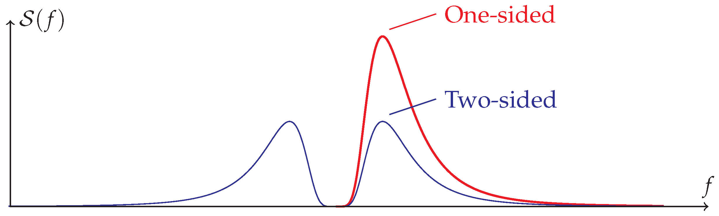
where $\mathcal{F}\left(x\right)$ is the Fourier transform of the function x, and $\left|\mathcal{F}\left(x\right)\right|$ denotes the absolute value of the given complex variable, in this case, $\mathcal{F}\left(x\right)$. Another point to note is that due to the symmetry of the Fourier transform’s result, the second half of $\mathcal{S}$ is equal to the first half, mirrored, thus the first half is usually multiplied by two and the second discarded, making the spectrum one-sided.

3. Transformation of the Spectrum

To transform the wave spectrum using the IFT it is necessary to first adequate the input of the algorithm so that its output is a real-valued function that represents the water surface height. It is known, from Axiom 1 of the Hermitian reciprocity relationship discussed in Section 2 that the water surface height, denoted henceforth by $\eta$, will only be a real-valued function if the Fourier transform of $\eta$, $\mathcal{F}\left(\eta \right)$, is a complex Hermitian function. In the case of $\mathcal{F}\left(\eta \right)$ being a Hermitian function, one can input it to the IFT algorithm to obtain $\eta$.

Usually, the spectrum is presented as a one-sided spectrum, in which case it has to be mirrored with respect to the frequency domain and divided by two, reversing the process previously described, as shown in Figure 1.

With the two-sided spectrum one can reverse Equation (2) to make $\mathcal{F}\left(x\right)$ explicit, which in the case at hand is $\mathcal{F}\left(\eta \right)$, and introduce, $\Delta f$, which roots from the frequency discretisation of the function:

$$\left|\mathcal{F}\left(\eta \right)\right|=\sqrt{{\mathcal{S}}_t\Delta f}$$

(3)

where ${\mathcal{S}}_t$ denotes specifically the two-sided spectrum.

The right-hand side of Equation (3) consists of just the original spectrum, rescaled by $\Delta f$, which is still a real-valued function because the product ${\mathcal{S}}_t\Delta f$ is always positive.

The only unknown left in Equation (3) is the absolute-value operator on $\mathcal{F}\left(\eta \right)$, which turns the complex-valued result of the Fourier transform into the real-valued right-hand side of Equation (3). Therefore, to remove the absolute-value operator of the equation, and make $\mathcal{F}\left(\eta \right)$ explicit, the right-hand side has to be made a complex-valued Hermitian function.

To complete the complex-valued function it is necessary to include the missing phase spectrum in Equation (3). Sea waves are modelled by their variance spectrum under the closure hypothesis that their phase spectrum is randomly and uniformly distributed in the interval $[0,2\pi ]$ [1,2,19], and the sea surface elevation due to such waves approximately fits a Gaussian distribution [19]. Adding up these two pieces makes it possible to assert that the missing phase spectrum can be modelled by a stream of normally-distributed random numbers with null average and unit standard deviation, with the same size (the length of the vector, denoted as n) as the original two-sided spectrum.

At this point, there are two real-valued functions, the amplitude and phase spectra, which need to be merged into one complex Hermitian function. As previously discussed, the real part of a Hermitian function is an even function and the imaginary part is odd.

Splitting the random number stream from before into two parts of the same size, $\alpha$ and $\beta$, and mirroring them with respect to the frequency domain as previously done for the spectrum, then changing the sign of the second half of $\beta$:

$$\begin{array}{cc}\hfill \alpha (n..n/2+1)& =+\alpha (1..n/2)\hfill \end{array}$$

(4a)

$$\begin{array}{cc}\hfill \beta (n..n/2+1)& =-\beta (1..n/2)\hfill \end{array}$$

(4b)

returns the real ($\alpha$) and imaginary ($\beta$) components of a complex Hermitian function. In Equations (4a) and (4b) the notation $a..b$ represents the integer range from a to b. If $a>b$ then the range is from b to a, reversed.

Finally, with $\alpha$ and $\beta$, the complex Hermitian function can be written as $\alpha +\mathrm{i}\beta$. Given that, Equation (3) can be rewritten with the Hermitian function in place and the Fourier transform of $\eta$ completely explicit:

$$\mathcal{F}\left(\eta \right)=\left[\alpha +\mathrm{i}\beta \right]\sqrt{{\mathcal{S}}_t\Delta f}$$

(5)

finally yielding a suitable definition for $\mathcal{F}\left(\eta \right)$, which now can be input to the IFT, resulting in the real-valued function $\eta$.

The generated time series of the water surface height, as computed with Equation (5), will be one random realisation of the wave spectrum used in the process. The variance spectrum will be embedded in the time series of $\eta$ as the amplitude of the oscillations, and the relative positions of such oscillations will reflect the random number stream used to generate the time series.

Reproducing the procedure with a different variance spectrum will produce a visually similar time series with changed amplitudes, while changing the random number stream will produce a rather different time series, but one which contains the same information when averaged over larger time scales.

An example implementation of the methodology to transform a water wave spectrum into a time series of surface elevation is available online: https://gist.github.com/PhelypeOleinik/39803f2385a18d0e86dc3ff8fe02af7b (accessed on 18 September 2021). The theoretical description of the methodology should cite this paper, and the code can be cited as:

Oleinik, P.H.; Tavares, G.P.; Machado, B.N.; Isoldi, L.A. Transformation of Water Wave Spectra into Time Series of Surface Elevation: base implementation. Earth 2021, 1, 1–9. Available online: https://gist.github.com/PhelypeOleinik/39803f2385a18d0e86dc3ff8fe02af7b (accessed on 18 September 2021).

4. Verification of the Method

The verification dataset for this method will be a set of 5000 discrete spectra from randomly selected points and time intervals from the simulation performed by Oleinik et al. [20]. Since this article does not feature a case study, this simulation was chosen only due to its relatively large space and time coverages to evaluate the method proposed here. The significant wave height of the sea states represented by the sampled spectra ranges between approximately 0.15 to  4 $\mathrm{m}$.

All the analyses in this section will use time series of $\eta$ generated from the sampled spectra above, each with 65,536 ($n=2^{16}$) points over a time interval of 3600 $\mathrm{s}$. The length of  1 $\mathrm{h}$ for the time series was chosen to be long enough to make statistical bias due to random numbers negligible, and to be short enough so that the sea state can be considered a stationary function in that period (although the latter would not influence here, since the usage of the spectrum already implies a stationary sea state).

Uniformly-distributed random number streams were generated using the GNU Fortran (5.4.0) random_number intrinsic function, which uses the xorshift1024∗ algorithm [21]. These were then transformed into normally-distributed random number streams using the polar form [22] of the Box–Muller transform [23].

4.1. Verification of Average Values

The first, most straightforward, verification of the proposed method is the fact that once the IFT is applied to the result of Equation (5), the imaginary part of the result is zero, as it should be to comply with Axiom 2 of the Hermitian reciprocity relationship from Section 2.

Another trivial verification is that, since the spectrum does not carry any information of the average sea surface height, the constant term of the Fourier transform is zero, therefore the average of $\eta$ is also zero. Figure 2 shows that the average of the time series for the sampled spectra is approximately zero. In fact, the residuals are below the precision limit for a double-precision variable, so it can be safely assumed as zero.

The most widely known and used spectral wave parameter is the significant wave height ($H_{\mathrm{s}}$). This parameter can be obtained by a number of different means. From the wave spectrum, the significant wave height is obtained from the zeroth-order moment ($m_0$) of the wave spectrum, which can be computed using the equation for the nth-order moment [24]:

$$m_n={\int }_0^{\infty }{f}^n\mathcal{S}\left(f\right)\mathrm{d}f$$

(6)

with $n=0$. Geometrically, $m_0$ represents the area under the graph of the spectrum, which can be proven by replacing $n=0$ in Equation (6), and $m_0$ also represents the total variance of the spectrum $\mathcal{S}\left(f\right)$. From $m_0$, the significant wave height can be approximated with [2]:

$$H_{m_0}=4.004\sqrt{m_0}$$

(7)

In this article, a simple integration with the Midpoint rule was used. Equation (7) is valid in this case because the wave phase spectrum is assumed to have a Gaussian distribution (see Section 3) and in the time scales used the sea state is considered stationary [1].

With $\eta$, the significant wave height can be computed using two different methods. The first is by computing the variance of $\eta$, which should be equal to the total variance of the spectrum, and is also computed using Equation (7), replacing $m_0$ bywith the variance of $\eta$ ($\sigma$). The second method is by using the zero up- or down-crossing methods, which consist in splitting a time series into individual waves, measuring their heights, and taking the average of the highest one-third of the wave heights.

The significant wave height was obtained from the 5000 spectra by evaluating Equation (7) with the total variance of each spectrum. The obtained values were taken to be the reference values of significant wave height for the following analyses since all results are derived from the spectra. The significant wave height of $\eta$ was then calculated using the aforementioned methods: using the variance of $\eta$ in Equation (7) to obtain $H_{\sigma }$, using the zero-up crossing method to obtain $H_{{}^1{/}_3\uparrow }$, and the zero-down crossing method to obtain $H_{{}^1{/}_3\downarrow }$.

Due to the amount of data a direct comparison of the four parameters does not provide a good measure of their correlation. The Pearson correlation coefficient (r) between $H_{m_0}$ (the significant wave height calculated from the spectra) and the other three metrics ranges between 0.9981 and 0.9985, and the linear regression coefficients are $A=1.0017$ (linear coefficient) and $B=-0.0032$ (intercept), so a scatter plot will not show much either.

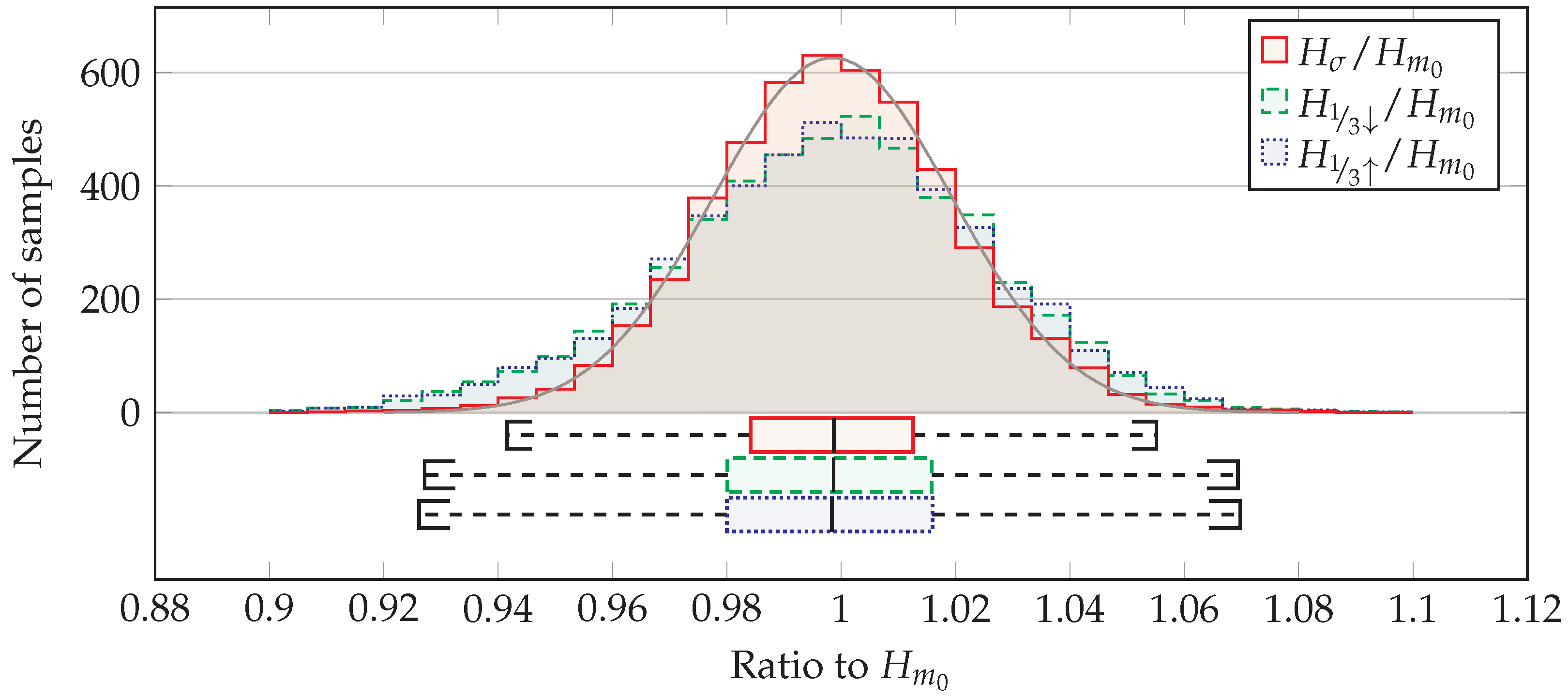
Therefore, the comparison of the three computed significant wave heights with $H_{m_0}$ was accomplished by taking the ratio between each of $H_{\sigma }$, $H_{{}^1{/}_3\uparrow }$, and $H_{{}^1{/}_3\downarrow }$, and the reference value $H_{m_0}$. Figure 3 shows the computed histogram of these ratios for the 5000 sampled spectra. The horizontal axis of Figure 3 represents the ratio between each of the analysed variables and the reference $H_{m_0}$. It represents how much the reference value is over- or under-estimated by each other method.

Figure 3 shows that $H_{\sigma }$ provides the best estimation of $H_{m_0}$ because it has more values closer to 1 (where $H_{\sigma }=$$H_{m_0}$). Both $H_{{}^1{/}_3\uparrow }$ and $H_{{}^1{/}_3\downarrow }$ yield slightly more scattered values, although the majority of the data points are still close to $H_{m_0}$. The better fitness of $H_{\sigma }$ is explained by the fact that it is computed using the variance of the variable of interest and Equation (7), as is $H_{m_0}$, so both are different measures of the same quantity. What makes $H_{\sigma }$ not identical to $H_{m_0}$ are the random number streams used in the generation of $\eta$ from the spectrum, as explained in Section 3.

$H_{{}^1{/}_3\uparrow }$ and $H_{{}^1{/}_3\downarrow }$ give more scattered values because they are not based on the variance of the sea surface elevation, as $H_{\sigma }$, they are derived from a different measurement of the surface height, so the estimate is not guaranteed to be the same. However the estimates of $H_{{}^1{/}_3\uparrow }$ and $H_{{}^1{/}_3\downarrow }$ are still mostly within 5% of $H_{m_0}$ and most of the fluctuation is possibly due to the random phase spectrum, as is the case with $H_{\sigma }$.

Below the histograms in Figure 3, the box plots show that on average all the estimates tend to the same value, as their ratio tends to 1. As expected, the estimation with $H_{\sigma }$ produces a narrower interquartile range, highlighting its higher accuracy. The box plots show that, except in the case of outliers, the significant wave height of the generated time series of $\eta$ will remain within 5% of the spectral significant wave height, thus showing that the transformation from the spectrum to the time series does not influence the underlying sea state.

It should also be noted that the distribution of $H_{\sigma }/$$H_{m_0}$ approximates a Gaussian distribution because the random number streams are normally distributed. The grey curve in Figure 3 shows a Gaussian curve fitted to the histogram of $H_{\sigma }/$$H_{m_0}$. The fitting resulted in a correlation coefficient of 0.9972.

4.2. Reversing the Process to Obtain the Spectrum from $\eta$

One final verification which can be made is whether after transforming the spectrum to a time series of $\eta$, this time series can be transformed back to the same spectrum. To reverse the process, Equation (5) has to be manipulated so that ${\mathcal{S}}_t$ is explicit on the left-hand side:

$${\mathcal{S}}_t=\Delta f^{-1}{\left(\frac{\mathcal{F}\left(\eta \right)}{\left[\alpha +\mathrm{i}\beta \right]}\right)}^2$$

(8)

where $\mathcal{F}\left(\eta \right)$ is the Fourier transform of $\eta$. However this approach uses the same random number streams $\alpha$ and $\beta$ as the forward transformation, and the result of ${\mathcal{S}}_t$ is trivial: the input spectrum.

In practical applications (data collected from a wave buoy, for instance) the phase spectrum (composed by $\alpha$ and $\beta$) is not available, only $\eta$ is. Equation (3), before the inclusion of the random number streams, directly relates ${\mathcal{S}}_t$ with $\eta$ through the Fourier transform. Rearranging Equation (3) to have ${\mathcal{S}}_t$ explicit:

$${\mathcal{S}}_t=\Delta f^{-1}{\left|\mathcal{F}\left(\eta \right)\right|}^2$$

(9)

results similar to Equation (8), but without $\alpha$ and $\beta$. It is worth noting that the absolute value operator which was removed from Equation (3) to obtain Equation (5) reappears here, after removing the random number streams.

Computing Equation (9) results in ${\mathcal{S}}_t$, a vector with the same number of elements as the time series of $\eta$. To obtain the one-sided spectrum, ${\mathcal{S}}_t$ should be truncated to the first $n/2$ elements (that is, half its length), and multiplied by two (see Figure 1).

To analyse the result of the process described above, one point was selected, taking into account the histogram in Figure 3, whose ratio $H_{\sigma }/$$H_{m_0}$ is approximately equal to one. Figure 4 shows the original spectrum, as described at the beginning of Section 4, taken from the point aforementioned. This spectrum was transformed into a 1 $\mathrm{h}$ long time series of $\eta$, using the methodology described in this article, and then Equation (9) was applied to this time series to obtain the spectrum from $\eta$.

However, it is clear from Figure 4 that, although the general behaviour of the result is consistent with the original spectrum, the direct application of Equation (9) is not enough to obtain the spectrum back due to the amount of noise in the result. This noise is intrinsic to the Fast Fourier Transform algorithm, which uses only one amplitude per frequency to estimate the variance density of the spectrum, yielding errors in the order of 100% [2].

One of the approaches to reduce this error is, instead of applying Equation (9) to the entirety of $\eta$ in one go, is to divide $\eta$ in a number (p) of non-overlapping segments, and then process each of these with Equation (9). The final spectrum is the frequency-wise average of each of these segments. This is referred to as the quasi-ensemble average of the spectrum [2], and it reduces the error by a factor of $\sqrt{p}$ at the expense of reducing the resolution of the data set by a factor of p. With a large enough time series of $\eta$, this should not be a problem, since the spectrum is usually discretised with around 50 frequencies, depending on the application.

Applying a quasi-ensemble average with $p=64$ segments to the data set being analysed reduces the error in the order of $12.5$%. Figure 4 also shows the final result after the noise reduction. It can be seen from Figure 4 that the result closely follows the original spectrum. The calculated root mean square error between the original spectrum and the result is $0.0198$ ${\mathrm{m}}^2$/$\mathrm{Hz}$.

5. Conclusions

In this article, a method is developed to transform a sea wave spectrum into a time series of sea surface elevation. The method is based on the definition of the variance spectrum from the result of a Fourier transform and uses the closure hypothesis that the phase spectrum of the waves is randomly distributed in the interval $[0,2\pi ]$. This allows providing both the amplitude and phase spectra to the IFT, which then returns the corresponding sea surface elevation.

The verification analyses of the method show that it is capable of correctly transforming a wave spectrum into a time series of sea surface elevation with maximum differences of around 5% due to the random phase spectrum inserted in the data. However, this difference in one realisation of the sea surface should not be considered as an error because, on average, it cancels out among other realisations. This difference is intrinsic to the usage of the spectrum as a predictor function for the sea surface elevation.

It should be noted, however, that the application of the IFT superimposes the individual components of the wave spectrum, without regard to nonlinear effects. Thus, for extreme sea states where the linear wave theory doesn’t hold, waves may be generated steeper than in reality, thus it is recommended attention be given to the generated results when applying this method to regions of very shallow water or extreme sea states. Further developments of this methodology may focus on detecting and avoiding these anomalies.

The methodology presented in this paper can be used to represent the sea state, provided the spectrum is known, in applications that require time-varying wave data, the most obvious one being the numerical modelling of wave flumes and tanks using CFD, but also as a boundary condition to other types of phase-solving wave models, and physical wave tanks. This method can also be used to generate wave data to simulate the load on offshore structures subject to wave action, or their fluid dynamic interactions, as done by Machado et al. [16], for example.

References

- Goda, Y. Random Seas and Design of Maritime Structures, 2nd ed.; Advanced Series on Ocean Engineering; World Scientific: Singapore, 2000; Volume 15. [Google Scholar]
- Holthuijsen, L.H. Waves in Oceanic and Coastal Waters, 1st ed.; Cambridge University Press: Cambridge, UK, 2007; p. 387. [Google Scholar]
- Boussinesq, J.V. Théorie des ondes et des remous qui se propagent le long d’un canal rectangulaire horizontal, en communiquant au liquide contenu dans ce canal des vitesses sensiblement pareilles de la surface au fond. J. Math. Pures Appl. 1872, 17, 55–108. [Google Scholar]
- Golden, K.M.; Bennetts, L.G.; Cherkaev, E.; Eisenman, I.; Feltham, D.; Horvat, C.; Hunke, E.; Jones, C.; Perovich, D.K.; Ponte-Castaneda, P.; et al. Modeling Sea Ice. Not. Am. Math. Soc. 2020, 67, 1. [Google Scholar] [CrossRef]
- Voermans, J.J.; Rabault, J.; Filchuk, K.; Ryzhov, I.; Heil, P.; Marchenko, A.; Collins, C.O., III; Dabboor, M.; Sutherland, G.; Babanin, A.V. Experimental evidence for a universal threshold characterizing wave-induced sea ice break-up. Cryosphere 2020, 14, 4265–4278. [Google Scholar] [CrossRef]
- Chen, W.; Dolguntseva, I.; Savin, A.; Zhang, Y.; Li, W.; Svensson, O.; Leijon, M. Numerical modelling of a point-absorbing wave energy converter in irregular and extreme waves. Appl. Ocean. Res. 2017, 63, 90–105. [Google Scholar] [CrossRef]
- Ransley, E.; Greaves, D.; Raby, A.; Simmonds, D.; Hann, M. Survivability of wave energy converters using CFD. Renew. Energy 2017, 109, 235–247. [Google Scholar] [CrossRef] [Green Version]
- Shen, Z.R.; Ye, H.X.; Wan, D.C. URANS simulations of ship motion responses in long-crest irregular waves. J. Hydrodyn. 2014, 26, 436–446. [Google Scholar] [CrossRef]
- Ferguson, T.M.; Fleming, A.; Penesis, I.; Macfarlane, G. Improving OWC performance prediction using polychromatic waves. Energy 2015, 93, 1943–1952. [Google Scholar] [CrossRef]
- Ferguson, T.M.; Penesis, I.; Macfarlane, G.; Fleming, A. A PIV investigation of OWC operation in regular, polychromatic and irregular waves. Renew. Energy 2017, 103, 143–155. [Google Scholar] [CrossRef]
- Horvat, C.; Tziperman, E. A prognostic model of the sea-ice floe size and thickness distribution. Cryosphere 2015, 9, 2119–2134. [Google Scholar] [CrossRef] [Green Version]
- Didenkulova, E.; Slunyaev, A.; Pelinovsky, E. Numerical simulation of random bimodal wave systems in the KdV framework. Eur. J. Mech. B/Fluids 2019, 78, 21–31. [Google Scholar] [CrossRef]
- Merigaud, A.; Ringwood, J.V. Free-Surface Time-Series Generation for Wave Energy Applications. IEEE J. Ocean. Eng. 2018, 43, 19–35. [Google Scholar] [CrossRef] [Green Version]
- Benoit, M.; Marcos, F.; Becq, F. Development of a Third Generation Shallow-Water Wave Model with unstructured spatial meshing. In Proceedings of the 25th International Conference on Coastal Engineering: Book of Abstracts, Orlando, FL, USA, 2–6 September 1996; American Society of Civil Engineers: New York, NY, USA, 1996; pp. 465–478. [Google Scholar]
- Awk, T. Tomawac User Manual Version 7.2. The Telemac-Mascaret Consortium. 2017. Available online: http://opentelemac.org (accessed on 18 September 2021).
- Machado, B.N.; Oleinik, P.H.; Kirinus, E.d.P.; dos Santos, E.D.; Rocha, L.A.O.; Gomes, M.d.N.; Paixão Conde, J.M.; Isoldi, L.A. WaveMIMO Methodology: Numerical Wave Generation of a Realistic Sea State. J. Appl. Comput. Mech. 2021, 7, 2129–2148. [Google Scholar] [CrossRef]
- Tavares, G.P.; Maciel, R.P.; dos Santos, E.D.; Gomes, M.N.; Rocha, L.A.O.; Machado, B.N.; Oleinik, P.H.; Isoldi, L.A. Estudo Numérico Comparativo da Potência Disponível Entre Ondas Regulares e Irregulares: Estudo de Caso de um Dispositivo de Coluna de Água Oscilante na Costa de Rio Grande–RS. Int. J. Dev. Res. 2021, 11, 23001. [Google Scholar] [CrossRef]
- Gentleman, W.M.; Sande, G. Fast Fourier Transforms—For Fun and Profit. In Proceedings of the Fall Joint Computer Conference on XX—AFIPS ’66, San Francisco, CA, USA, 7–10 November 1966; ACM Press: New York, NY, USA, 1966; p. 563. [Google Scholar] [CrossRef]
- Cavaleri, L.; Alves, J.H.; Ardhuin, F.; Babanin, A.; Banner, M.; Belibassakis, K.; Benoit, M.; Donelan, M.; Groeneweg, J.; Herbers, T.; et al. Wave modelling—The state of the art. Prog. Oceanogr. 2007, 75, 603–674. [Google Scholar] [CrossRef] [Green Version]
- Oleinik, P.H.; Kirinus, E.d.P.; Cristiano, F.; Marques, W.C.; Costi, J. Energetic Potential Assessment of Wind-Driven Waves on the South-Southeastern Brazilian Shelf. J. Mar. Sci. Eng. 2019, 7, 25. [Google Scholar] [CrossRef] [Green Version]
- Marsaglia, G. Xorshift RNGs. J. Stat. Softw. 2003, 8. [Google Scholar] [CrossRef]
- Knop, R.E. Remark on algorithm 334 [G5]: Normal random deviates. Commun. ACM 1969, 12, 281. [Google Scholar] [CrossRef]
- Box, G.E.P.; Muller, M.E. A Note on the Generation of Random Normal Deviates. Ann. Math. Stat. 1958, 29, 610–611. [Google Scholar] [CrossRef]
- Mackay, E. Resource Assessment for Wave Energy. In Comprehensive Renewable Energy; Elsevier: Amsterdam, The Netherlands, 2012; Volume 8, pp. 11–77. [Google Scholar] [CrossRef]
Figure 1.
Illustration of the one-sided and two-sided representation of the same spectrum.
Figure 2.
Mean values of the time series of the 5000 sampled spectra for the verification.
Figure 3.
Histogram and box plot of the ratio between , , and and the reference for the 5000 sampled spectra.
Figure 4.
Wave spectra at the point selected for analysis. “Original” is the original spectrum used for the analysis, “Equation (9)” is the result of Equation (9) applied on the time series of obtained from the original spectrum, and “Result” is the result of Equation (9) after noise removal treatment.
Publisher’s Note: MDPI stays neutral with regard to jurisdictional claims in published maps and institutional affiliations. |
© 2021 by the authors. Licensee MDPI, Basel, Switzerland. This article is an open access article distributed under the terms and conditions of the Creative Commons Attribution (CC BY) license (https://creativecommons.org/licenses/by/4.0/).
Share and Cite
MDPI and ACS Style