
Capitalization and Capital Return in Boreal Carbon Forestry


Lehtoi Research, 81235 Lehtoi, Finland
Earth 2022, 3(1), 204-227; https://0-doi-org.brum.beds.ac.uk/10.3390/earth3010014
Submission received: 1 January 2022
/
Revised: 26 January 2022
/
Accepted: 2 February 2022
/
Published: 7 February 2022
Abstract
:In this paper, an attempt is made to determine an intangible capitalization premium based on an expected further value increment of forest stands. Such premium cannot be determined through exponential interpolation. Firstly, any discount rate depending on maturity proposes clearcuttings soon after thinning as a computational artifact. Secondly, exponential interpolation with a constant discount rate violates an internal consistency criterion as the rotation age increases. Omitting the intangible capitalization premium, the carbon stock of boreal forest can be increased in a variety of ways (albeit at the expense of a capital return rate deficiency). A small excess volume can be economically gained by increasing sapling density. Greater excess volume is best achieved by restricting thinnings. A large excess volume is best achieved by omitting thinnings. Regardless of the technique used, enhanced carbon storage requires financial compensation in terms of a carbon rent. With the present European emission prices, there is no financial difficulty in establishing such a carbon rent arrangement.
1. Introduction
There are two large sinks of atmospheric carbon on planet Earth: the oceans and the forests [1,2,3,4]. It is difficult to manipulate oceans, whereas forests can be managed. By definition, a carbon sink is a system with a positive time change rate of stored carbon. This paper discusses the microeconomics of boreal forests as a carbon sink.
A particular benefit of the boreal forest is carbon storage in the soil. The amount of soil carbon may exceed the carbon storage in living biomass [5,6,7,8,9,10]. However, living biomass produces litter resulting in soil carbon accumulation and, consequently, the rate of carbon storage depends on the rate of biomass production on the site. The biomass production rate is related to the amount of living biomass [6,9,11,12]. As the time change rate of storage constitutes a sink, this paper focuses on changes in living biomass. In the case of trees, one of the most straightforward indicators of living biomass per surface area unit is the commercial volume of tree trunks.
The outcome of any process depends on the essential contributing mechanisms. Such mechanisms can often be described in terms of a process model. However, the outcome also depends on the occurring initial conditions, or more broadly, boundary conditions. In real-life applications, the initial conditions vary. Results of model-based investigations can be considered robust (or non-chaotic) if they are coherent under realistically varying sets of initial conditions [13]. In this paper, two different sets of initial conditions are used.
The objective functions discussed in this paper are partially microeconomic and partially of a physical character. The microeconomic objective function is the capital return rate [14,15,16,17,18]. The physical objective functions are carbon storage area densities, discussed in terms of living biomass, and measured in area densities of commercial trunk volumes.
There is a hierarchy between the objective functions. Firstly, the capital return rate is maximized. Then, deviations are introduced, and the relationship of capital return rate deficiency to excess commercial volume is investigated. The deviations are introduced in terms of additional sets of boundary conditions. These are constituted by sets of restrictions applied to intermediate harvesting practices or, in other words, thinning restrictions. Some of the restrictions may result in a favorable combination of carbon storage and capital return deficiency, in which case the deficiency could be compensated in terms of a carbon rent [19]. In addition to thinning restrictions, selection of sapling density retained after young stand tending is discussed, as well as the selection of tree species.
There are many previous investigations discussing the economic feasibility of thinning practices [20,21,22,23,24,25,26,27,28]. Some of them also discuss carbon storage features [9,12,29,30,31]. However, a few studies contain deficiencies restricting their applicability. Common deficiencies are unrealistic assumptions regarding the yield of various timber assortments, as well as pricing assumptions not adhering with reality [31,32,33,34,35]. It also appears that the optimal number of thinnings, thinning intensity, as well as selection between continuous-cover forestry and clearcuttings, depend on the applied discounting interest rate [20,21,22,23,24,25,26,27,28].
The capital return rate in forestry has been investigate sparsely [14,15,16,17,18,36,37]. Results regarding the relationship of capital return rate and carbon storage are still more sparse [14,15,16,17,18]. Again, some of the available results are deficient due to unrealistic yield assumptions [17,38]. Others have used financial boundary conditions not considered appropriate in this investigation [14,18]. There is an earlier study discussing capital return rate deficiency per excess volume unit appearing with the intent of carbon storage where the financial boundary condition meets that one here considered appropriate [15]. That study, however, did not discuss eventual thinning restrictions in detail [15].
In this paper, capital return rate and forest stand capitalization are discussed from the viewpoint of carbon storage and carbon sequestration. First, we present the financial techniques applied, as well as a few ways of determining forest stand capitalization. We attempt to include an intangible asset in the capitalization. Then, we apply two different datasets in the determination of stand capitalization and the corresponding capital return rate. Firstly, a growth model is applied in young stands as early as the inventory-based model is applicable. Secondly, the growth model is applied to observed wooded stands. Finally, the effect of management practices on the relationship between carbon storage and capital return rate is discussed. Three different thinning practices are discussed, as well as sapling density and choice of tree species.
2. Materials and Methods
2.1. Financial Considerations
We apply a procedure first mentioned in the literature in 1967, but applied only recently [14,15,16,17,18,36,37]. Instead of discounting revenues, the capital return rate achieved as relative value increment at different stages of forest stand development is weighed by current capitalization, and integrated.
The capital return rate is the relative time change rate of value. We choose to write
where in the numerator considers value growth, operative expenses, interests and amortizations, but neglects investments and withdrawals. In other words, it is the change of capitalization on an economic profit/loss basis. K in the denominator gives capitalization on a balance sheet basis, being directly affected by any investment or withdrawal. Technically, K in the denominator is the sum of assets bound on the property: bare land value, value of trees, and non-amortized value of investments. In addition, intangible assets may appear. The pricing of forest estates may include goodwill value. The intangible asset discussed in this paper is a premium applied to young stands due to their expected further value growth.
The momentary definition appearing Equation (1) provides a highly simplified description of the capital return rate. In reality, there is variability due to a number of factors. Enterprises often contain businesses distributed to a variety of production lines, geographic areas, and markets. In addition, quantities appearing in Equation (1) and are not necessarily completely known but may contain probabilistic scatter. Correspondingly, the expected value of capital return rate and valuation can be written, by definition,
where corresponds to the probability density of quantity i.
Let us then discuss, the determination of capital return rate in the case of a real estate firm benefiting from the growth of multiannual plant stands of varying ages. Conducting a change of variables in Equation (3) results as
where a refers to stand age. Equation (3) is a significant simplification of Equation (2) since all probability densities now discuss the variability of stand age. However, even Equation (3) can be simplified further.
In Equation (3), the probability density of stand age is a function of time, and correspondingly the capital return rate, as well as the estate value, evolve in time. A significant simplification would appear if the quantities on the right-hand side of Equations (2) and (3) would not depend on time. Within forestry, such a situation would be denoted “normal forest principle”, corresponding to evenly distributed stand age determining relevant stand properties [39].
The “normal forest principle” is rather useful when considering silvicultural practices, but seldom applies to the valuation of real-life real estate firms, with generally non-uniform stand age distribution. However, it has recently been shown [40] that the principle is not necessary for the simplification of Equation (3) into (4). This happens by focusing on a single stand, instead of an entire estate or enterprise, and considering that time proceeds linearly. Then, the probability density function p(a) is constant within an interval [0, τ]. Correspondingly, it has vanished from Equation (4).
2.2. Determination of Stand Capitalization
There is a variety of methods to determine the value K appearing in Equations (1)–(4). In the case of an incorporated company or a firm with equivalent reporting, an estimate can be found from the balance sheet. Such an outcome does depend on applied accounting practices. On the other hand, the value can be determined as a market value. The latter is straightforward in the case of publicly listed companies, or other companies with established share trading records. A third alternative for firm value determination is the computation of an “intrinsic value”, considering the prognosticated future development of the firm [41,42,43].
In the case of a real estate firm benefiting from the growth of multiannual plants of varying age, the asset value K within any stand may be approached as the sum of the value of the plants on the stand, the value of bare land, and the value of non-amortized investments. Such computation may be problematic if non-mature plants do not have any immediate sales value. In such a case, it is not uncommon to determine stand value by discounting expected future revenues [21,22,23]. The discount rate is sometimes taken arbitrarily, but often it can be determined as an internal rate of return [44]. Such discounting typically results as an intangible expectation premium in valuation, added to the immediate sales value of components.
Here, we provide a few examples of the determination of the value of forest stands by interpolation. It is not uncommon that planted seedlings may require several years to mature to young trees of commercial value. However, during those years, expected revenues become closer in time. Correspondingly, it would be unrealistic to assume the growth of saplings would not add value. The capitalization, including growth expectation premium, can be approximated by a smoothing function. One possibility could be
where r(t) is the capital return rate at stand age t, and τ is rotation age. A simpler version would be
Both of the above Equations converge to terminal capitalization , regardless of the capital return rate r(t) or . However, there is no guarantee of any definite convergence in a newly established stand. Such convergence could be approached by fitting an internal rate of return i which provides convergence. That would correspond to assuming that the bare land value includes any additional expectation value for a newly established stand, resulting as
It might be possible to determine capitalization indirectly by discounting revenue. This would result as
where BL denotes bare land value, and R(t) net revenue at time t. Again, the discount rate j shall be fitted for convergence .
Equations (6)–(8) above contain an apparently constant discount rate. In money market theory, increased duration of commitments tends to increase the risk experienced by the lender [45,46,47]. This could be considered by introducing a delay-dependent discount rate. One possibility is a spot discount rate
where d is time to maturity, and u and s are constants. Now, the constants u and s can be adjusted to gain the correspondence in Equation (8). On the other hand, it is only the constant u that determines the discount rate at maturity, and that can be determined through matching terminal discount rate to terminal capital return rate, determined as the ratio of terminal value increment rate to terminal capitalization. The terminal capital return rate, however, may depend on short-range disturbances such as thinning of forest stands. In particular, shortly after thinning, the capital return rate may be elevated; Equation (9) might contain negative values of s. Temporarily elevated capital return rate after thinning would reduce the estimate of capitalization, increase estimated capital return rate, and propose clearcutting soon after thinning (obviously a computational artifact). Such problems could be avoided by taking the constant u as the minimum short-term capital return rate appearing within a rotation. However, even this solution is problematical since the observable momentary capital return rate may be very low in young stands of saplings.
An important internal consistency criterion must be applied to Equations (5)–(9). A straightforward approximation for the current capitalization, excluding any intangible expectation premium, is
K(a) = bare land value + value of trees + value of non-amortized investments
The last term depends on investment intensity, as well as the amortization schedule. For the purposes of the internal consistency criterion, we define reduced current capitalization as
K′(a) = bare land value + value of trees
Approximations of capitalization established in Equations (5)–(9) are designed to include expectations of forthcoming value increment. Consequently, one can take for granted
A brief examination revealed that Equations (5)–(7) generally do not satisfy this internal consistency criterion and must thus be rejected. Equation (8), applied with or without Equation (9), often does satisfy the consistency criterion. However, this does not happen in all circumstances. Particularly, Equation (8) with a constant discount rate fails to comply with Equation (12) with large rotation ages.
Determining capitalization through the interpolation procedure given in Equation (8) does not require any knowledge of amortization schedule of investments. Instead, application of Equation (10) does require a definite amortization schedule. Here, with Equation (10), regeneration expenses are capitalized at the time of regeneration and amortized at the end of any rotation [15].
2.3. The Two Datasets Applied
The two different sets of initial conditions have been described in three earlier investigations [14,15,40]. Firstly, a group of nine setups was created computationally, containing three tree species and three initial sapling densities [15]. The idea was to apply the inventory-based growth model as early in stand development as it is applicable, to avoid approximations of stand development not grounded on the inventory-based growth model [48]. This approach also allowed an investigation of a wide range of stand densities, as well as a comprehensive description of the application of three tree species. The exact initial conditions here equal the ones recommended in [15].
The second set of initial conditions contains seven wooded, commercially unthinned stands located in Vihtari, Eastern Finland, first observed at the age of 30 to 45 years. The total stem count varied from 1655 to 2451 per hectare. A visual quality approximation was implemented. The number of stems deemed suitable for growing further varied from 1050 to 1687 per hectare. The basal area of the acceptable-quality trees varied from 28 to 40 m2/ha, in all cases dominated by spruce (Picea abies) trees.
3. Results
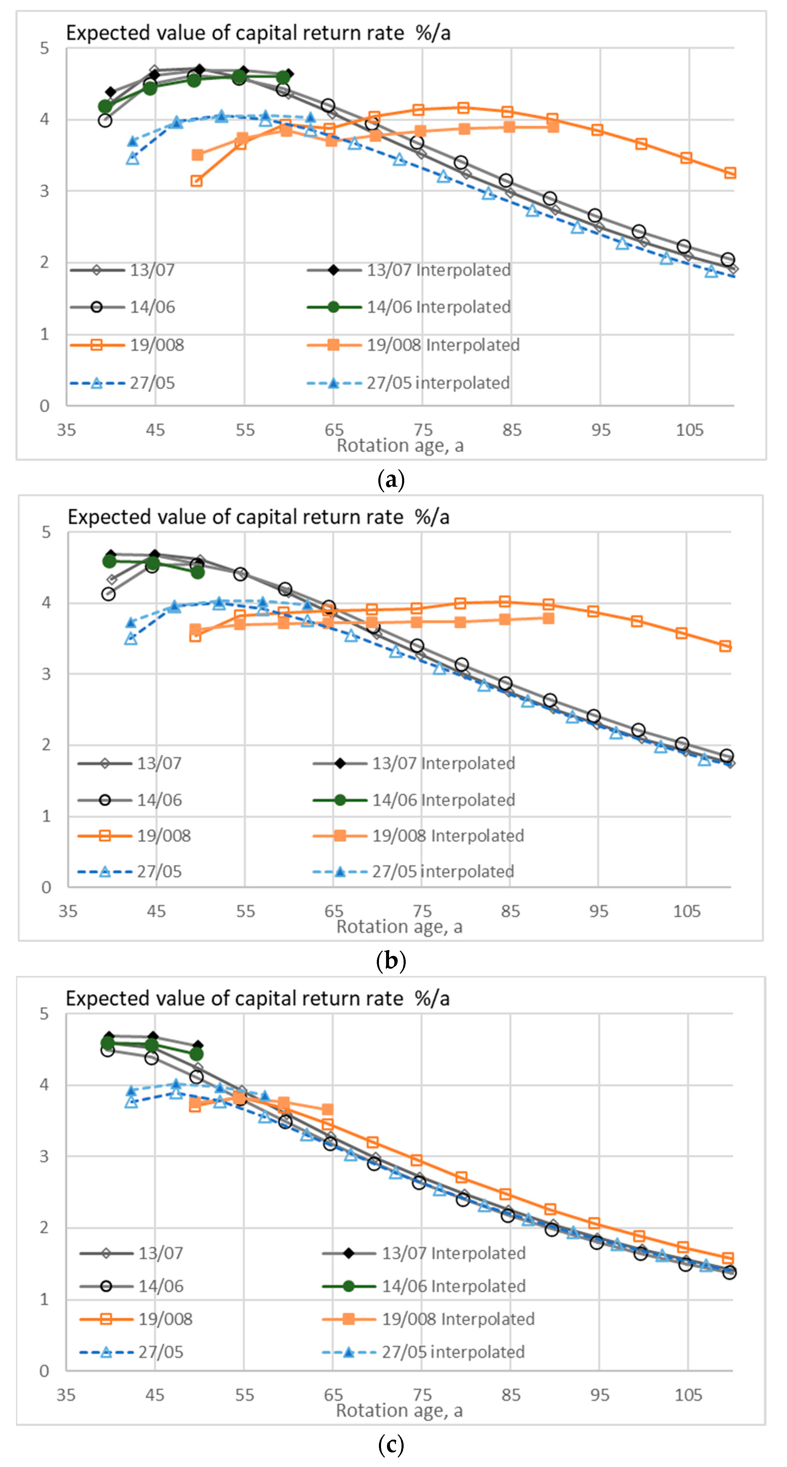
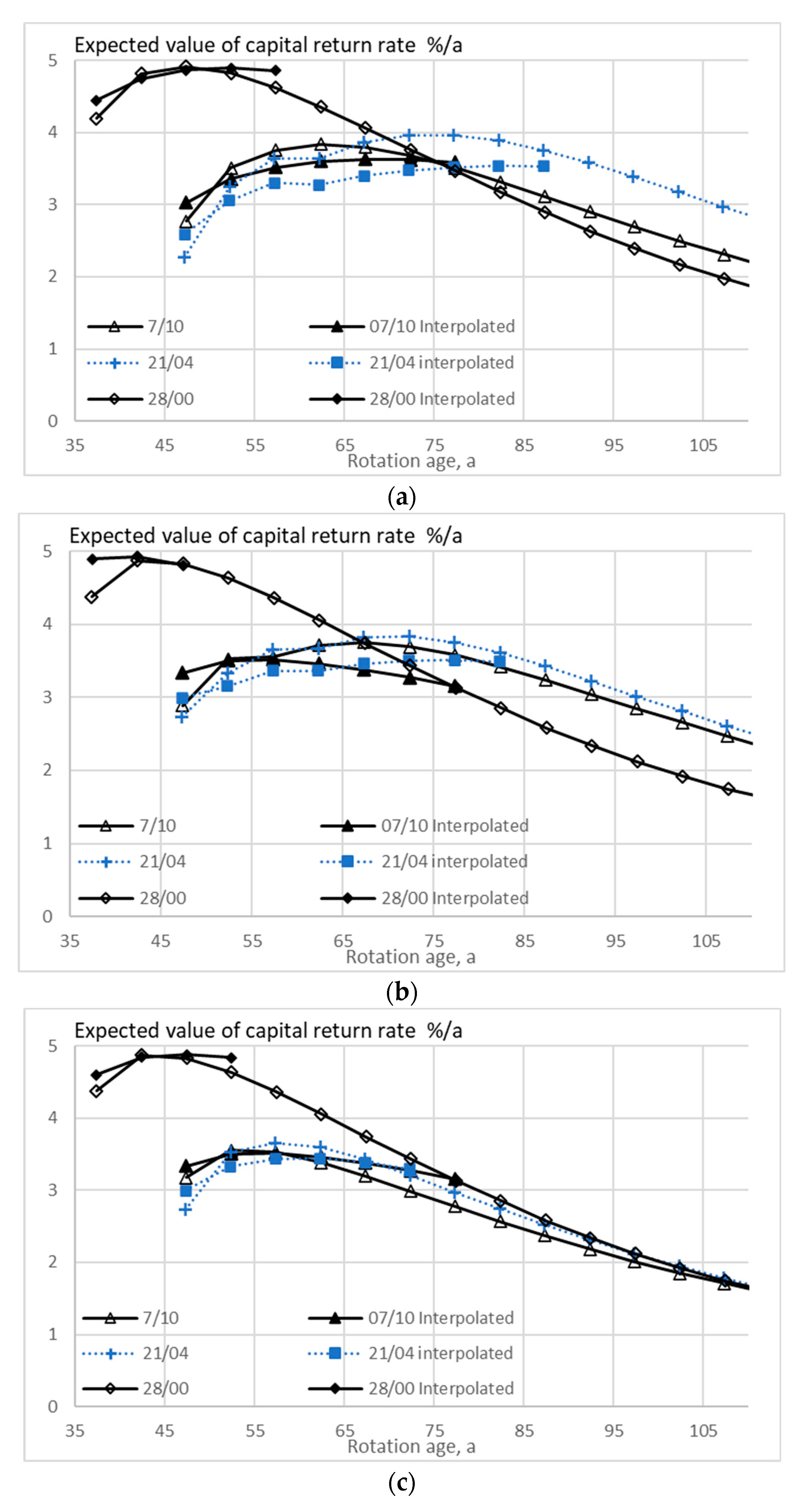
Figure 1 and Figure 2 show the expected value of the capital return rate within seven stands first observed at the age of 30 to 45 years, in the presence of eventual thinning restrictions. Thinning restrictions somewhat reduce the capital return rate and shorten rotation times. Application of Equation (8) in the determination of capitalization, instead of Equation (10), usually lengthens rotation times but does not affect the achievable capital return rate much. Long rotation times are not achievable using the interpolation Formula (8) since the internal consistency condition (12) becomes violated with increasing rotation age.
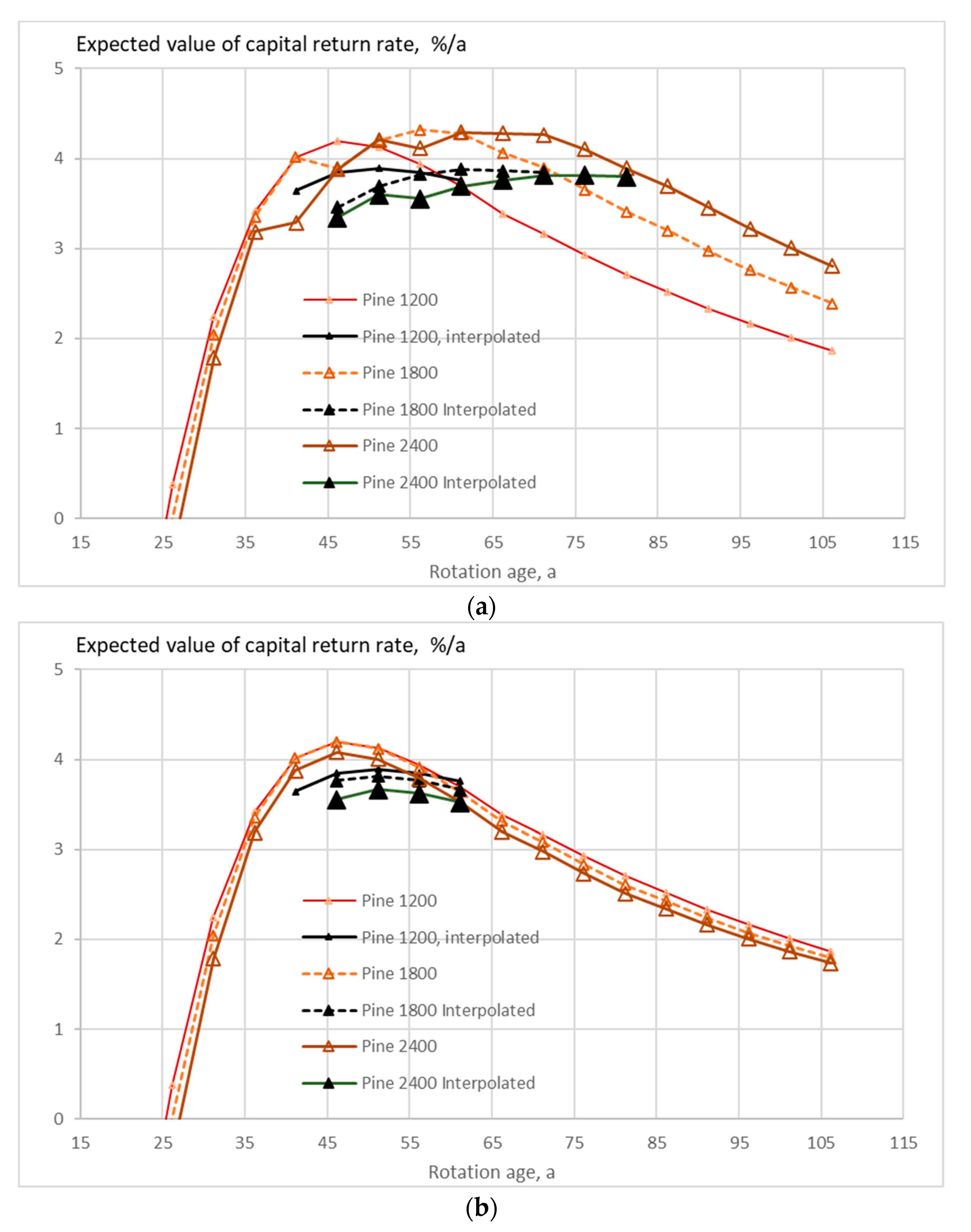
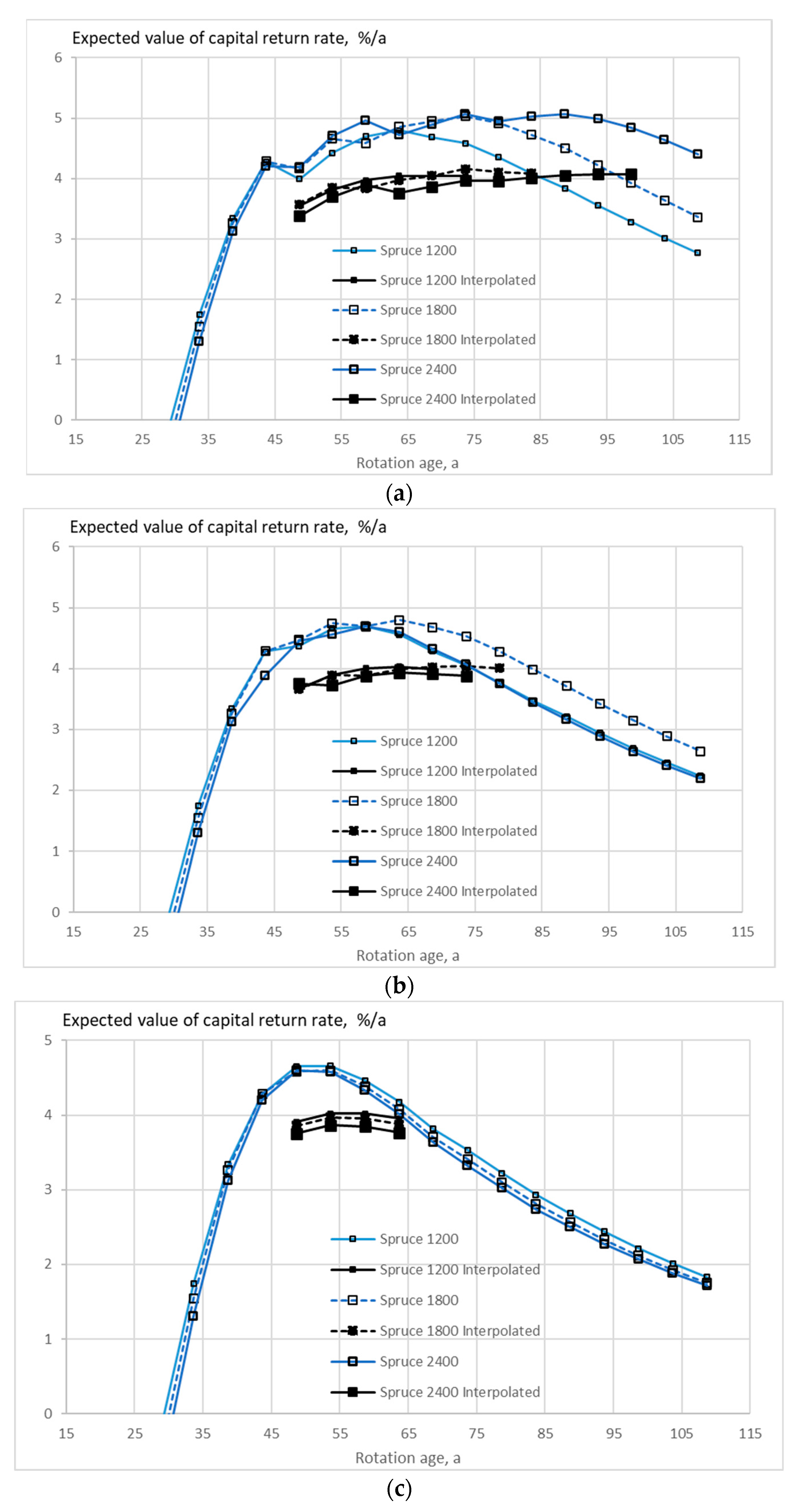
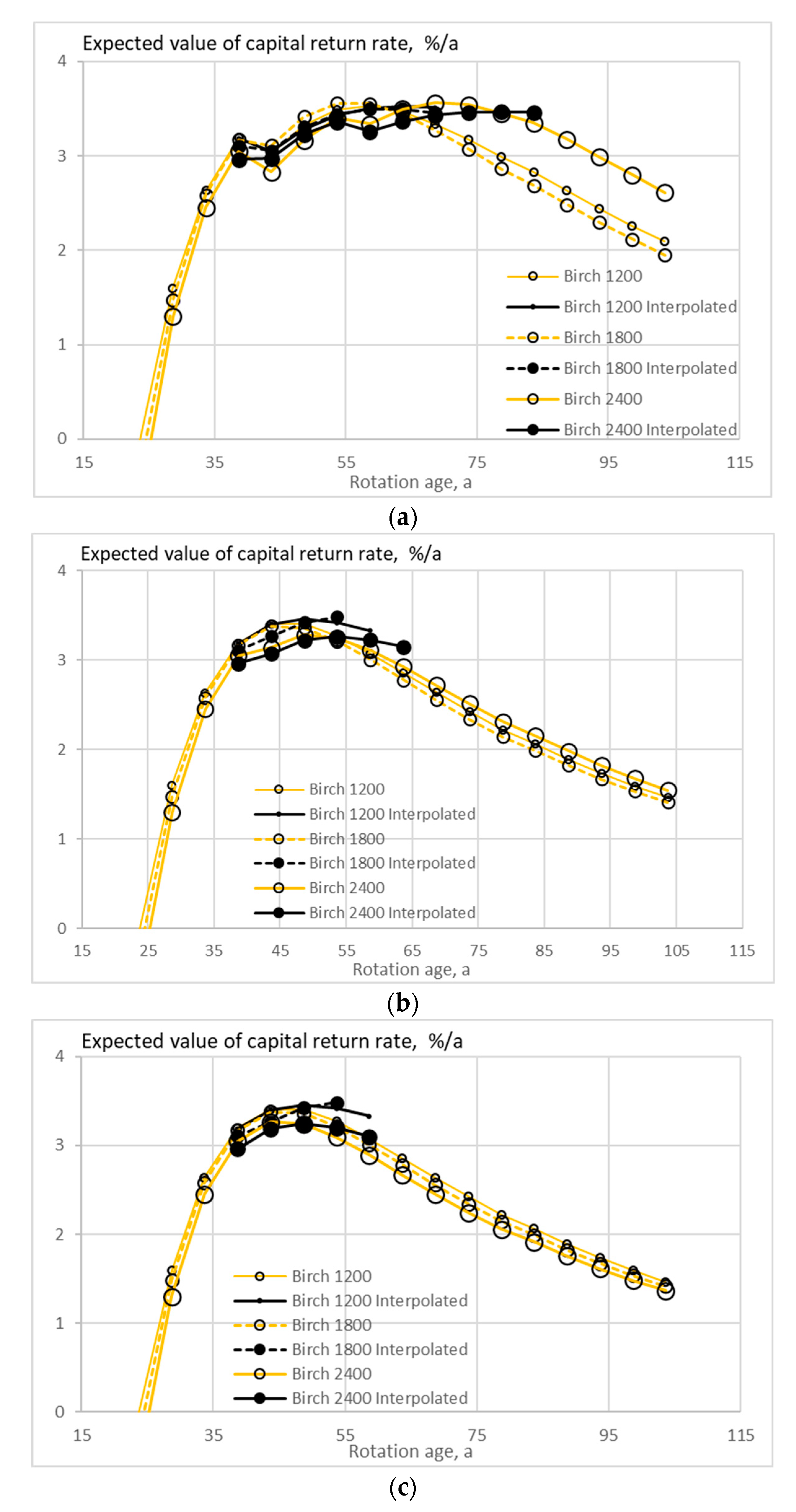
Figure 3, Figure 4 and Figure 5 show the expected value of the capital return rate within stands of three tree species where the growth model is applied as early as applicable. It is found that rotation times maximizing capital return rate become the shorter the stronger are the thinning restrictions. Rotation times are generally extended by the application of the interpolative formula (8) instead of (10). In the case of conifers, capital return rates become lower when Equation (8) is used. Long rotation times are not achievable using the interpolation Formula (8) since the internal consistency condition (12) becomes violated with increasing rotation age.
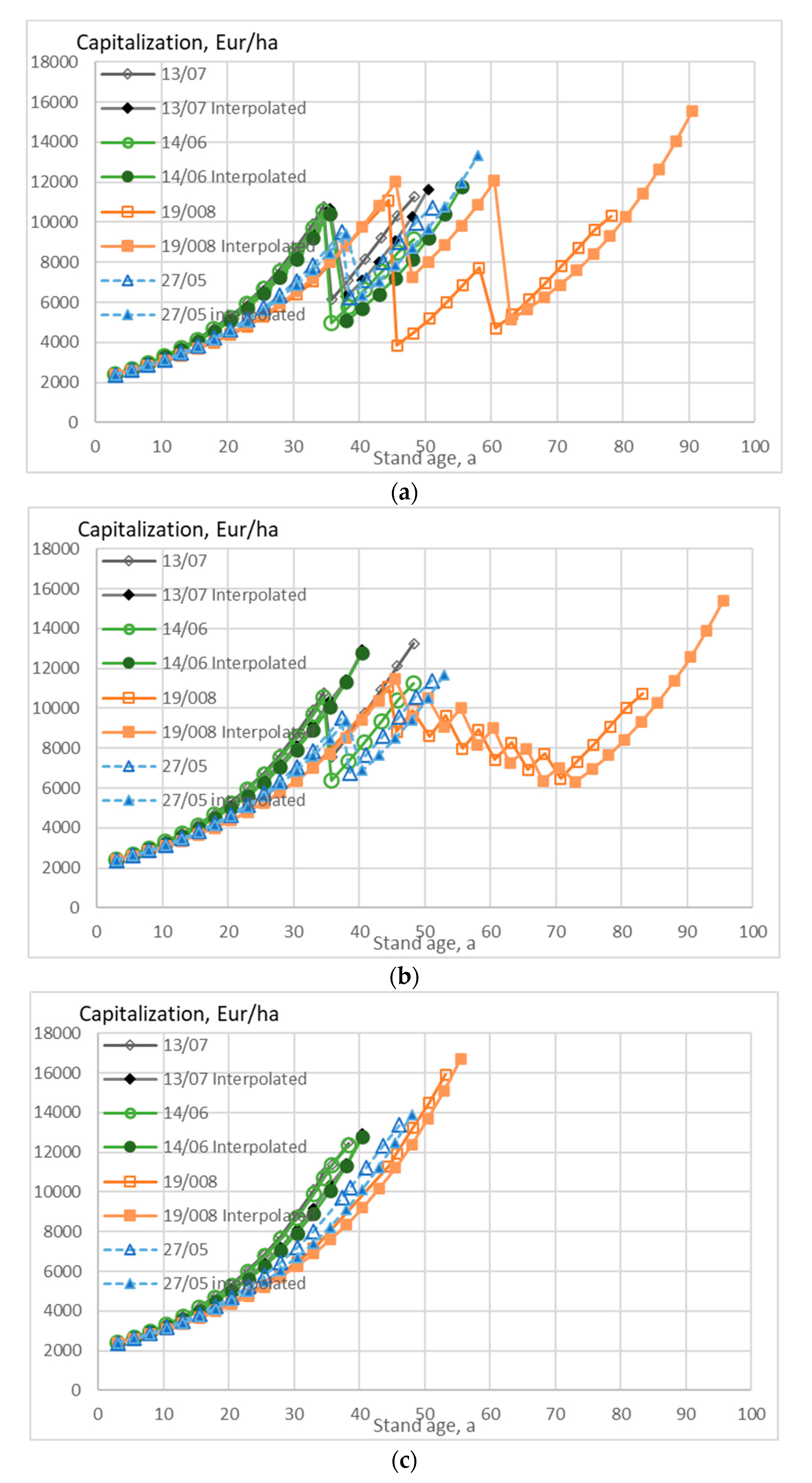
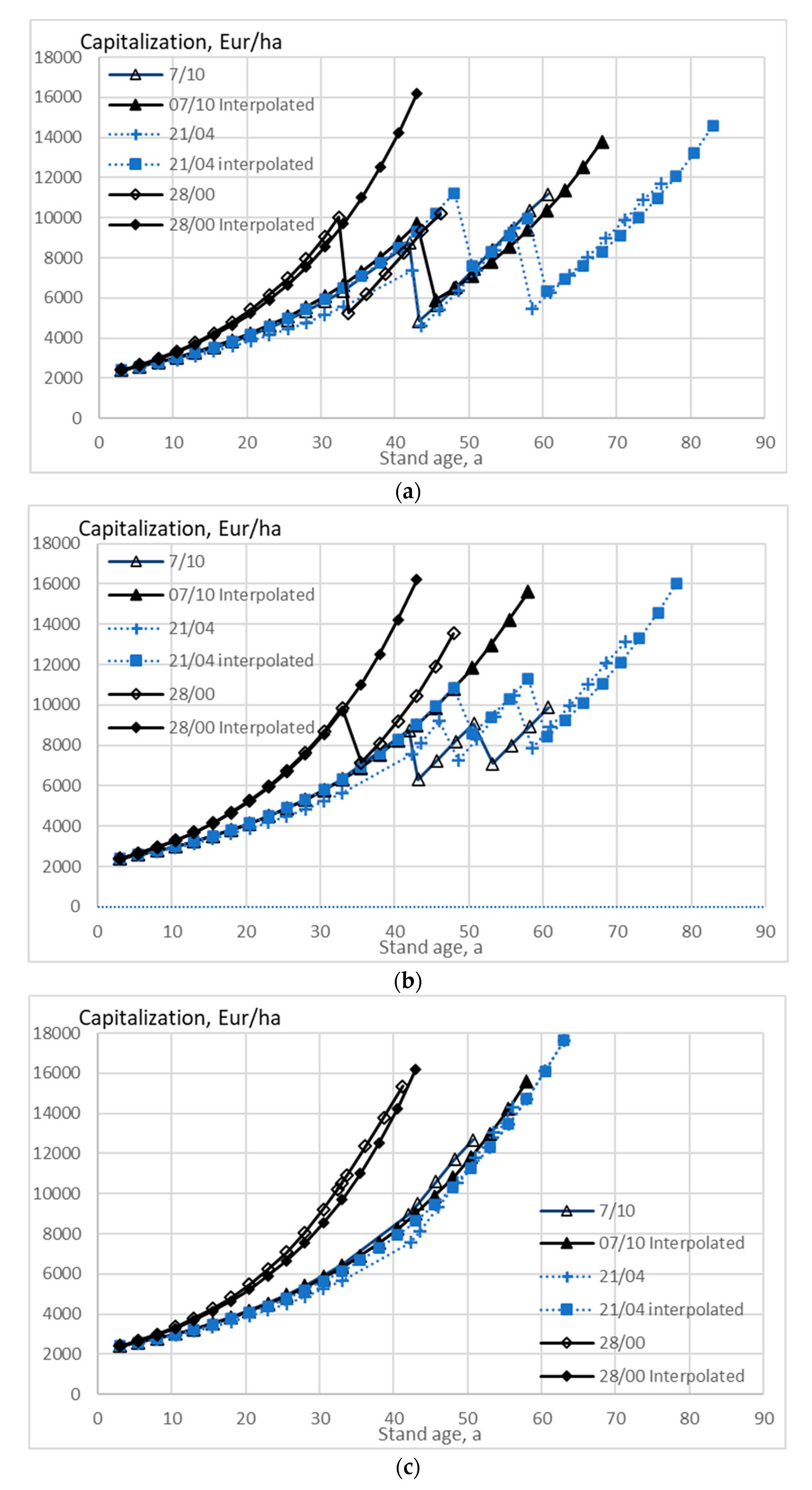
Figure 6 and Figure 7 show the stand capitalization as a function of stand age within seven stands first observed at the age of 30 to 45 years in the presence of eventual thinning restrictions. Again, thinning restrictions shorten rotation times. Application of Equation (8) in the determination of capitalization, instead of Equation (10), usually lengthens rotation times and requires somewhat gentler thinnings (and sometimes the omission of thinnings). Both the longer rotation time and the gentler thinning increase capitalization.
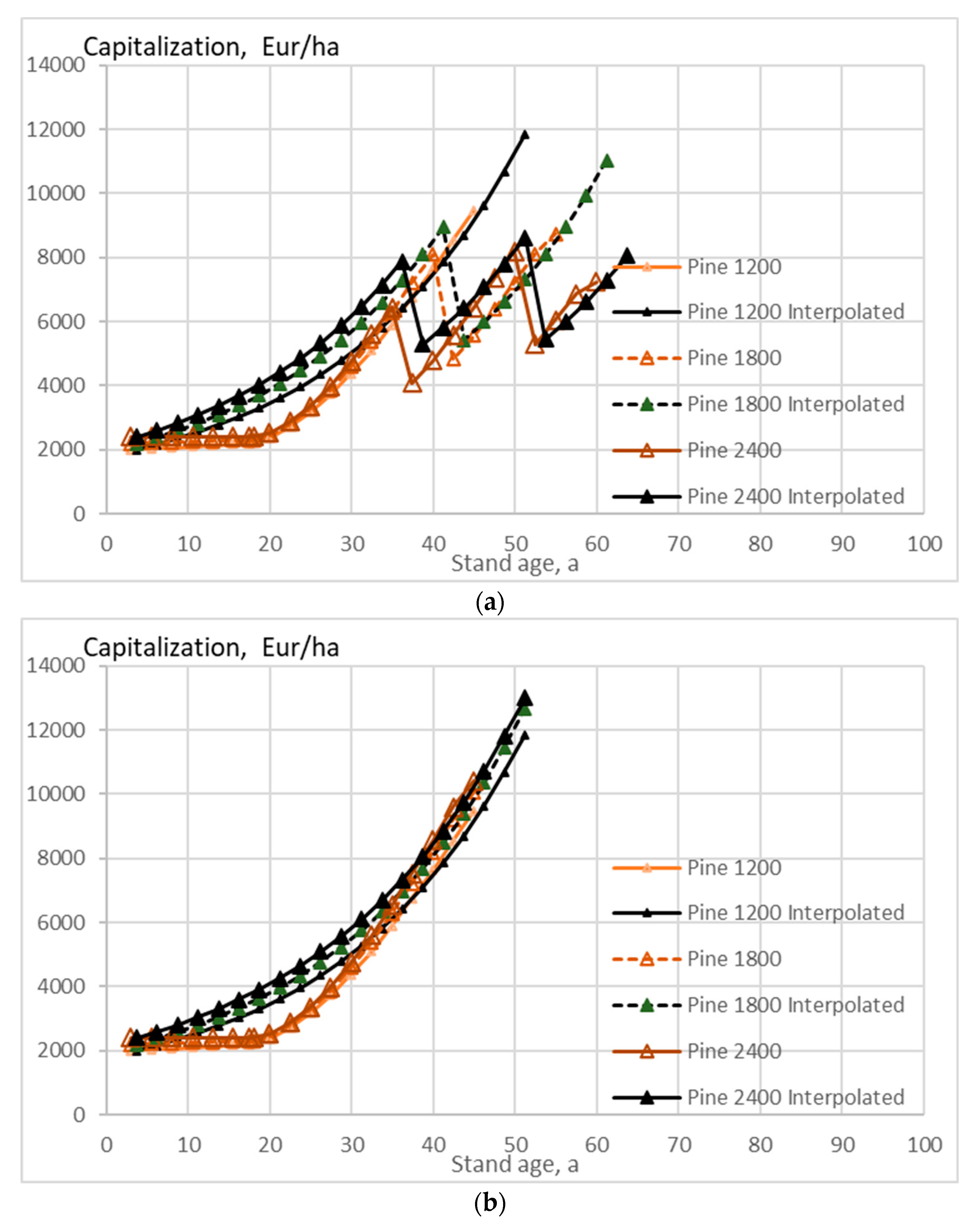
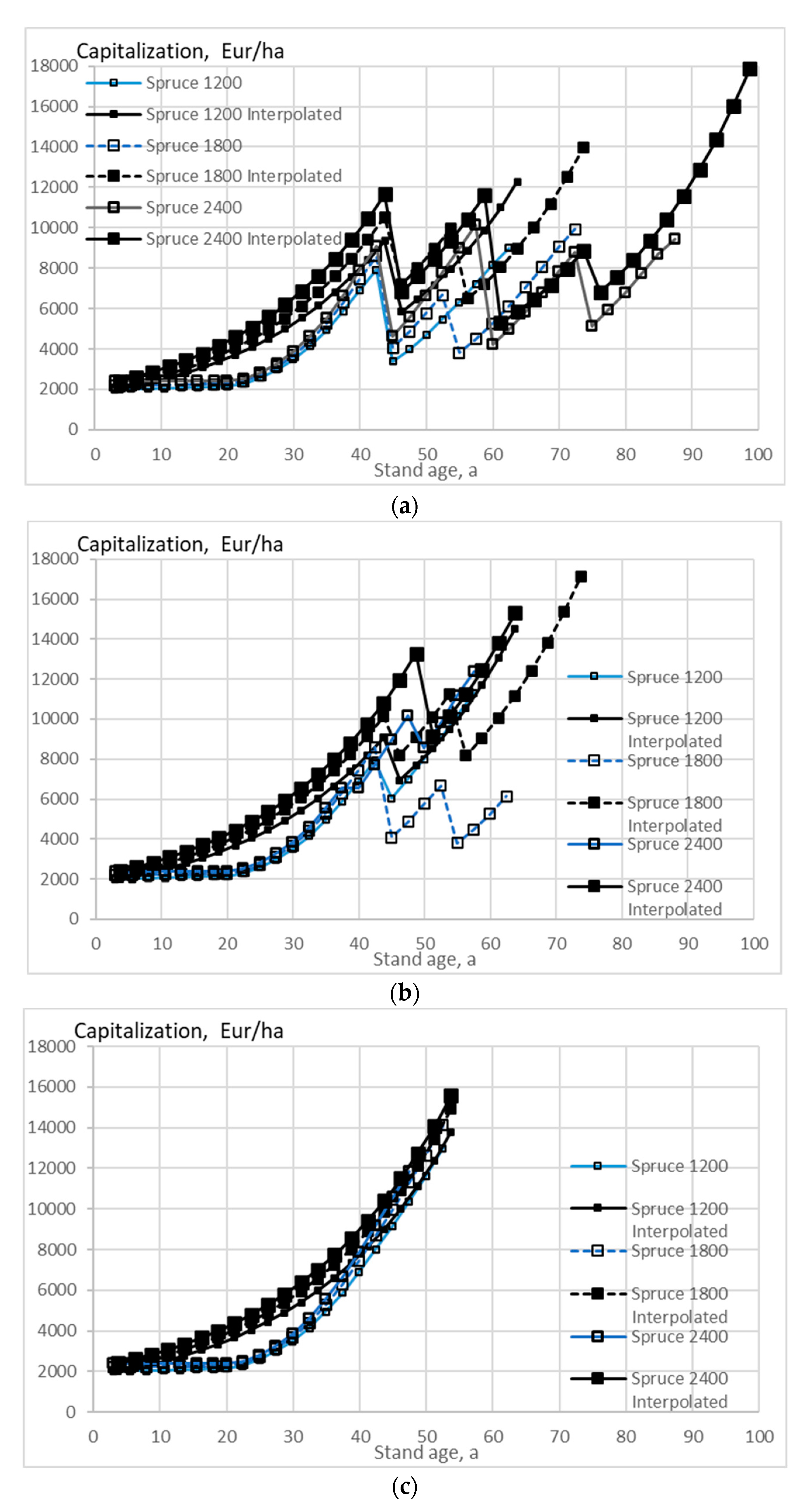
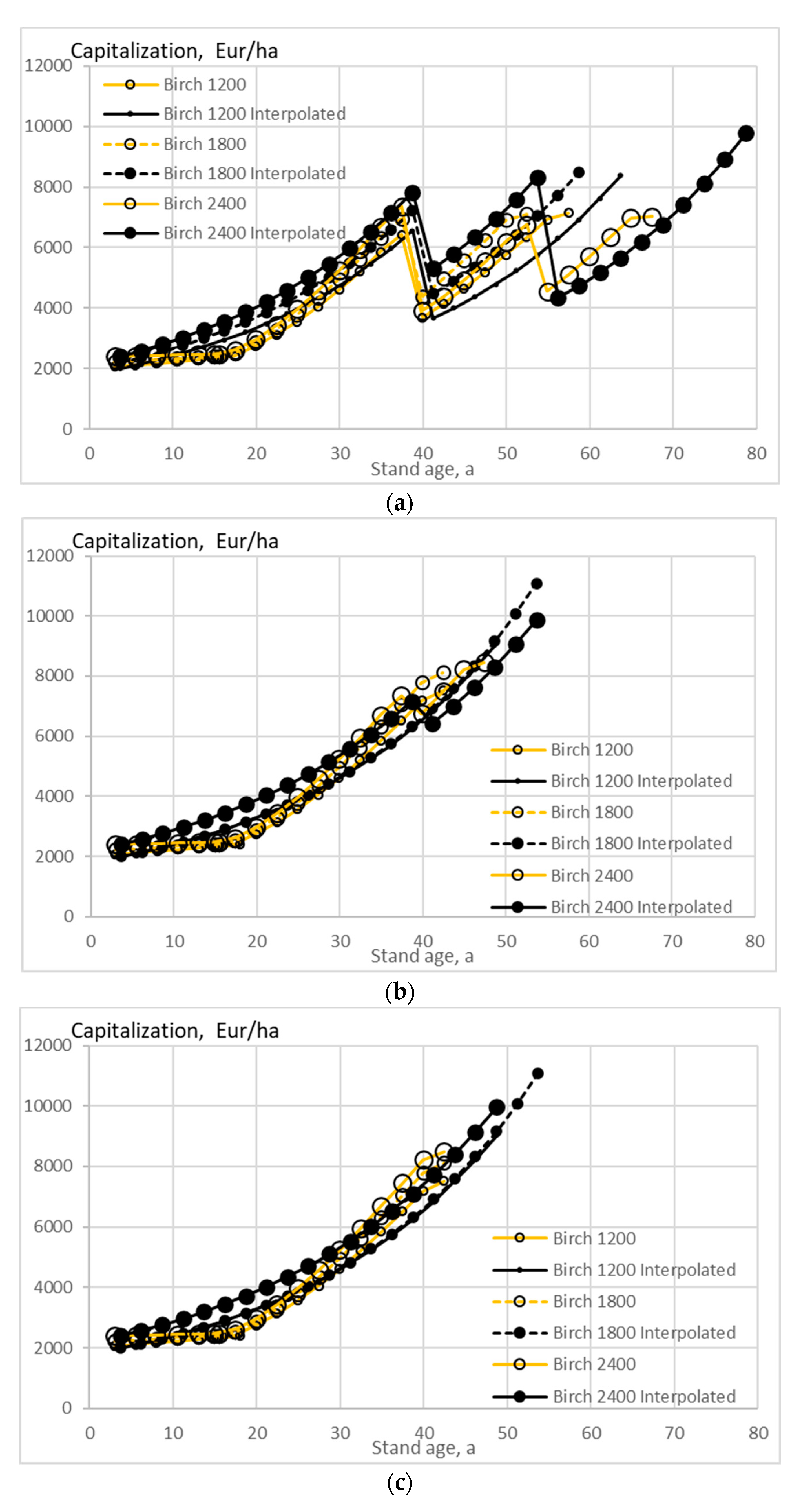
Figure 8, Figure 9 and Figure 10 show the stand capitalization as a function of stand age within stands of three tree species where the growth model is applied as early as applicable, in the presence of eventual thinning restrictions. Again, thinning restrictions shorten rotations. It is also found that thinning restrictions increase capitalizations. Again, the application of Equation (8) in the determination of capitalization, instead of Equation (10), lengthens rotation times, requires gentler thinnings. and increases capitalizations, the latter being affected by both gentler thinnings and longer rotation times.
Any deviation from the procedures corresponding to the maximum capital return rate induces a deficiency in capital return rate. Annual monetary deficiency per hectare can be gained by multiplying the deficiency in percentage per annum by current capitalization per hectare. Any deviation from the procedures corresponding to the maximum capital return rate also changes the expected value of the volume of trees per hectare. In case the volume is greater than that volume corresponding to the maximum capital return rate, there is a positive expected excess volume (also a negative excess volume may appear). The annual monetary deficiency per hectare can be divided by the excess volume to yield a measure of the financial burden of increasing the timber stock.
Figure 11 shows the expected value of the capital return rate deficiency per excess volume unit as a function of excess volume, within seven stands first observed at the age of 30 to 45 years, in the presence of eventual thinning restrictions. Thinning restrictions reduce the deficiency and increase available excess volume. Thinnings restricted to trees larger than 237 mm diameter show the smallest deficiency with moderate excess volume, while the omission of thinnings shows the smallest deficiency at large excess volumes. Application of Equation (8) in the determination of capitalization, instead of Equation (10), produces only small values of excess volume. Large excess volumes are not achievable using the interpolation Formula (8) since the internal consistency condition (12) becomes violated with increasing rotation age.
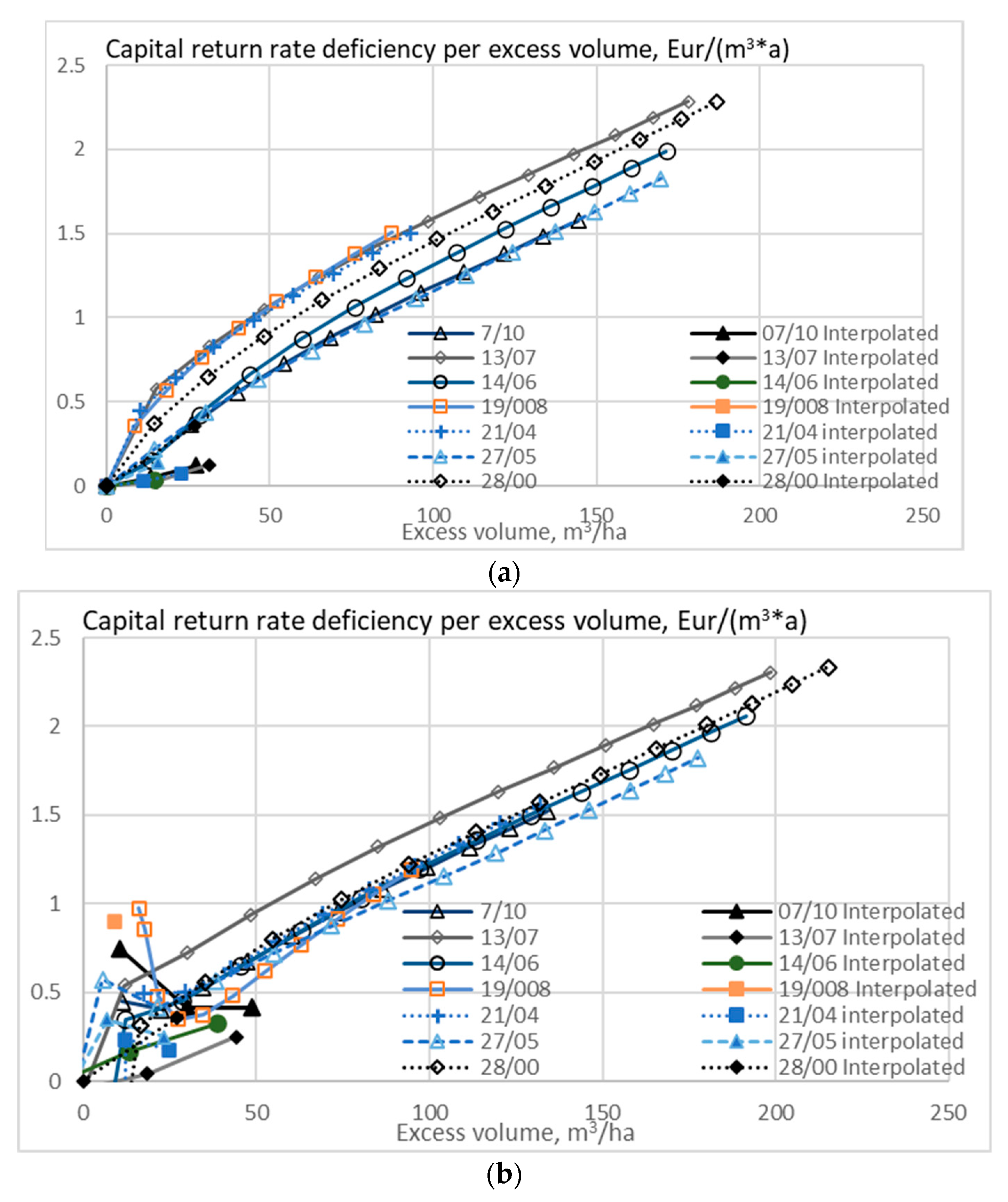
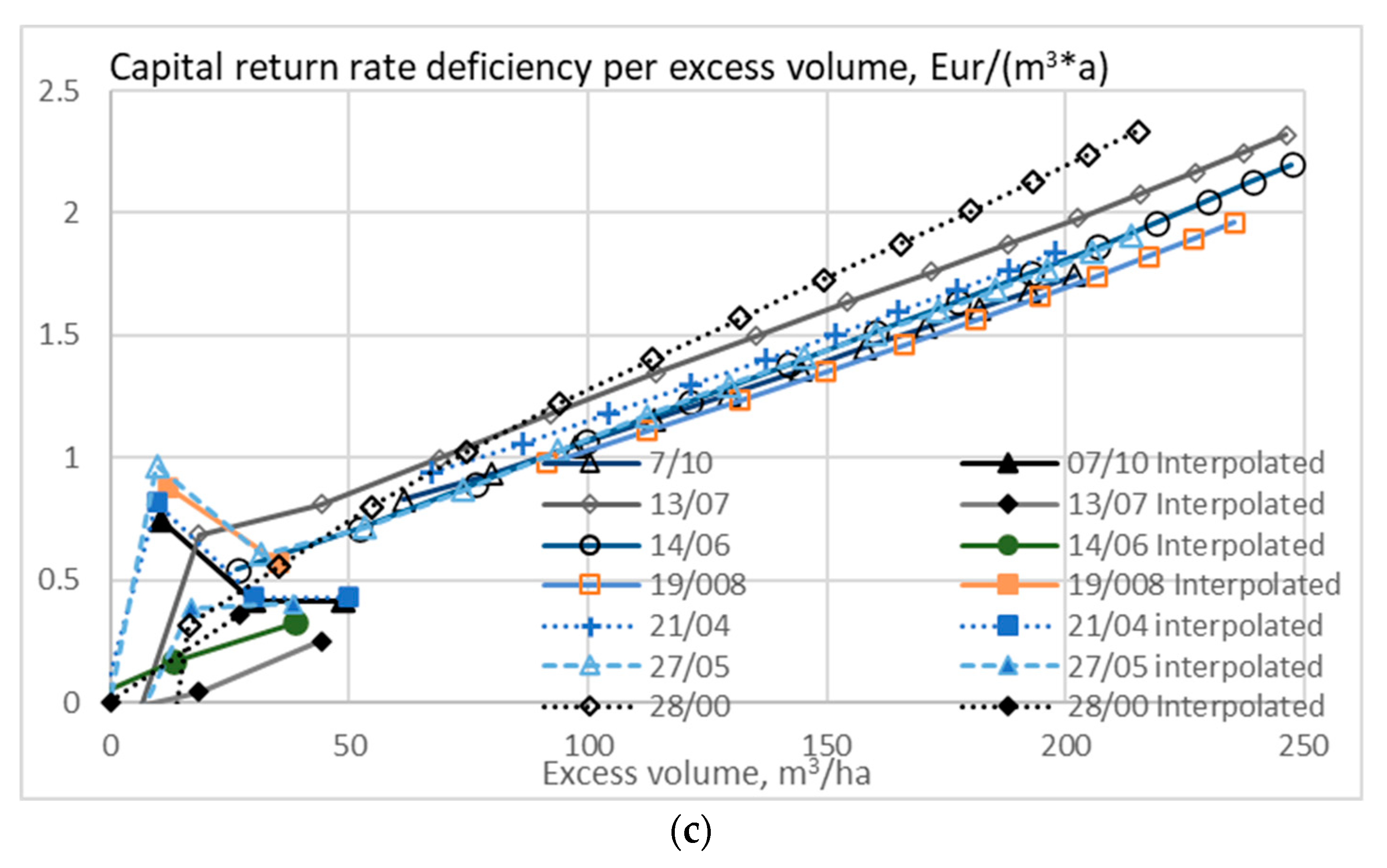
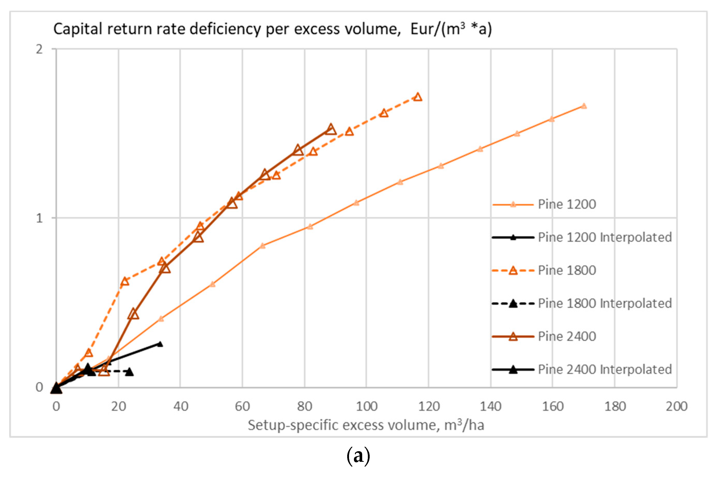
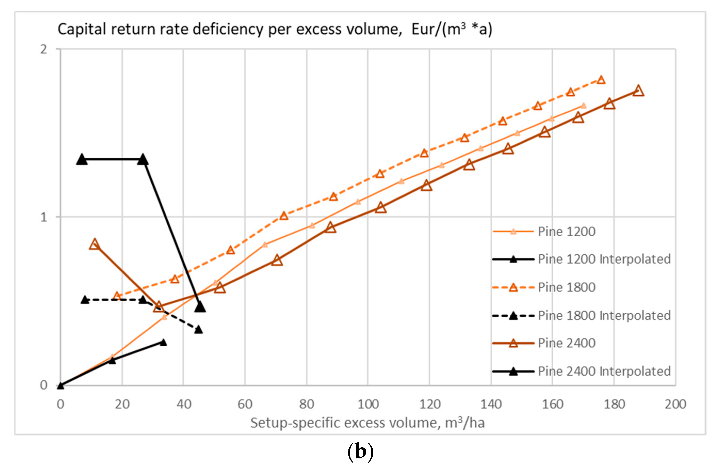
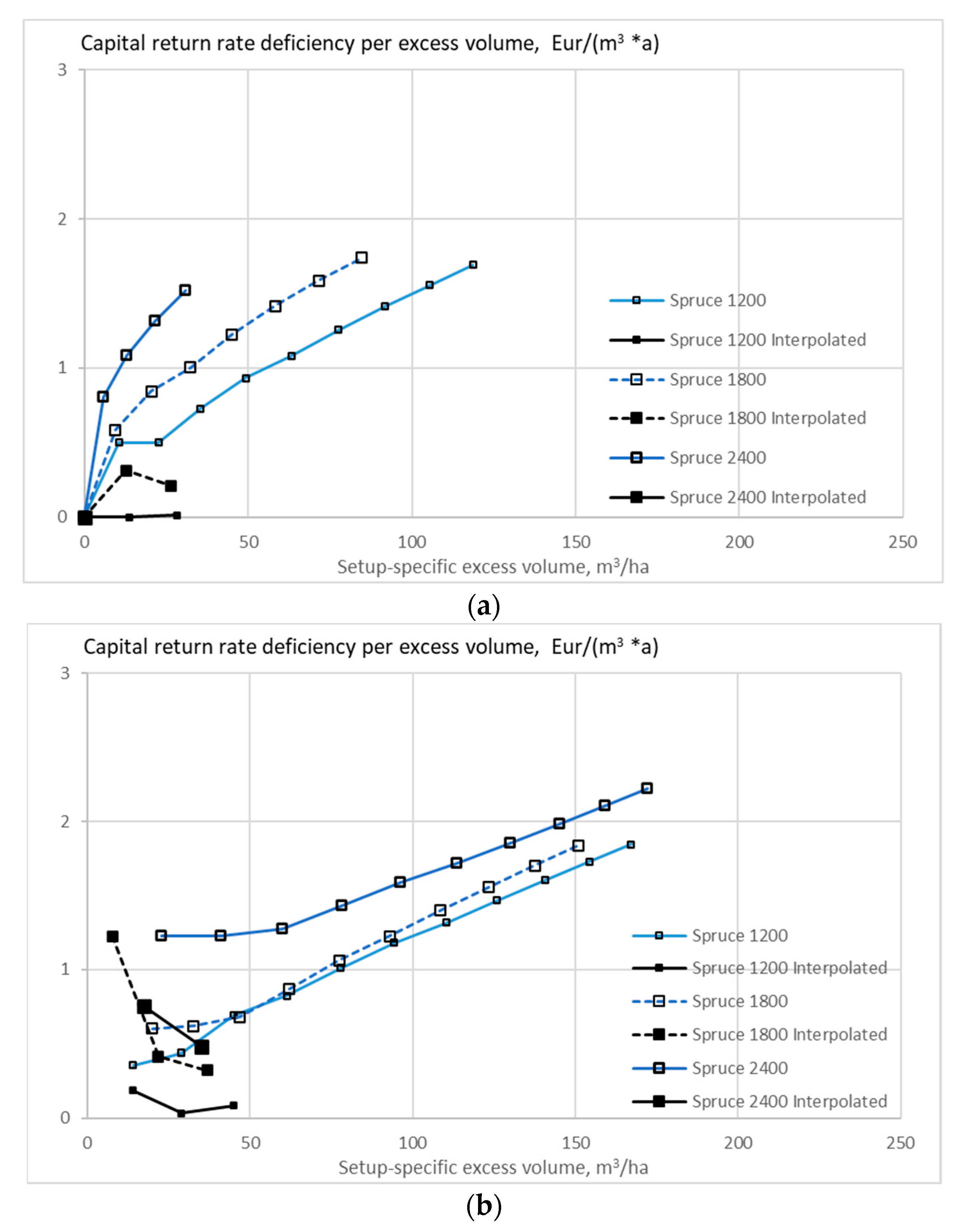
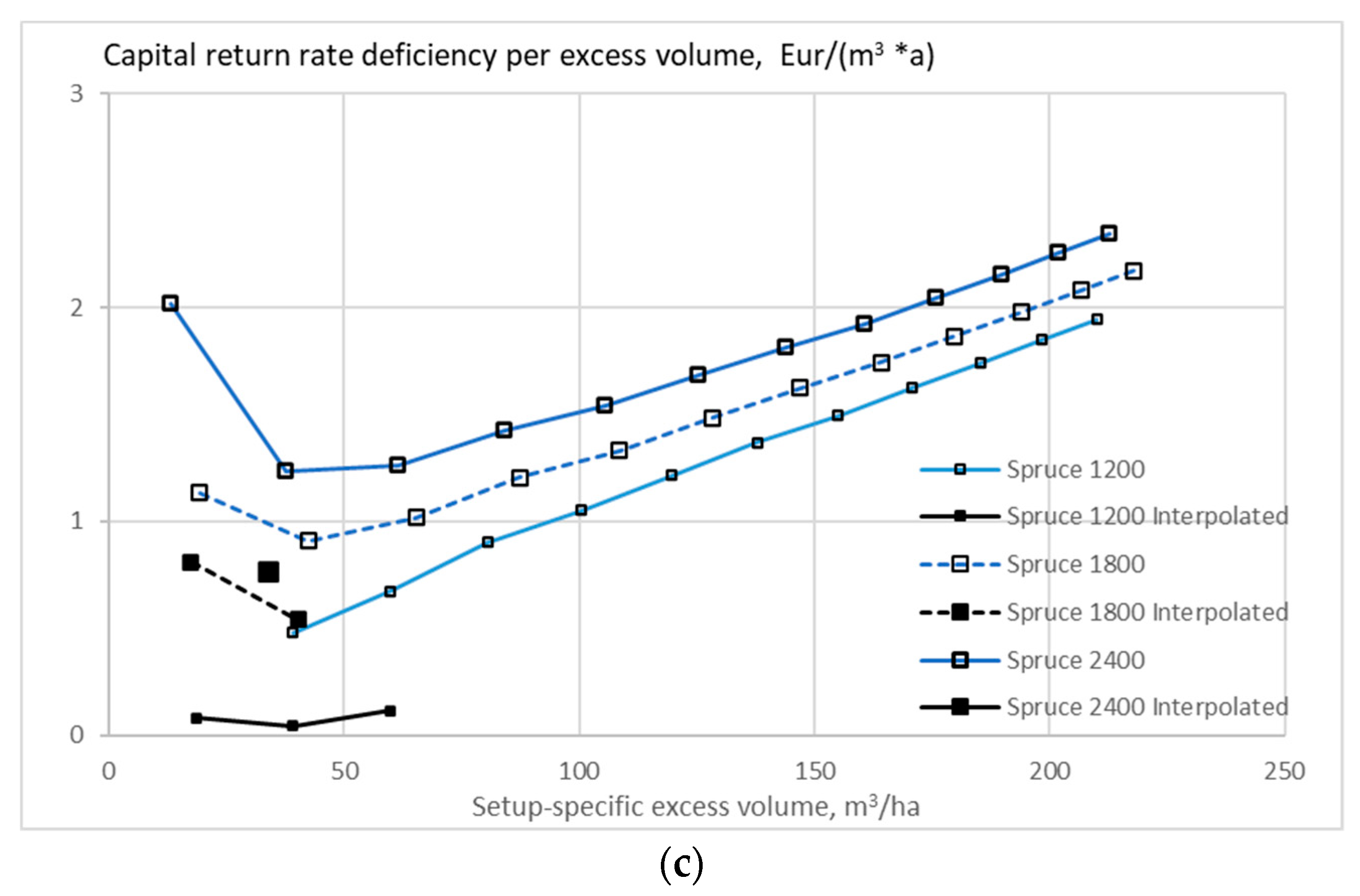
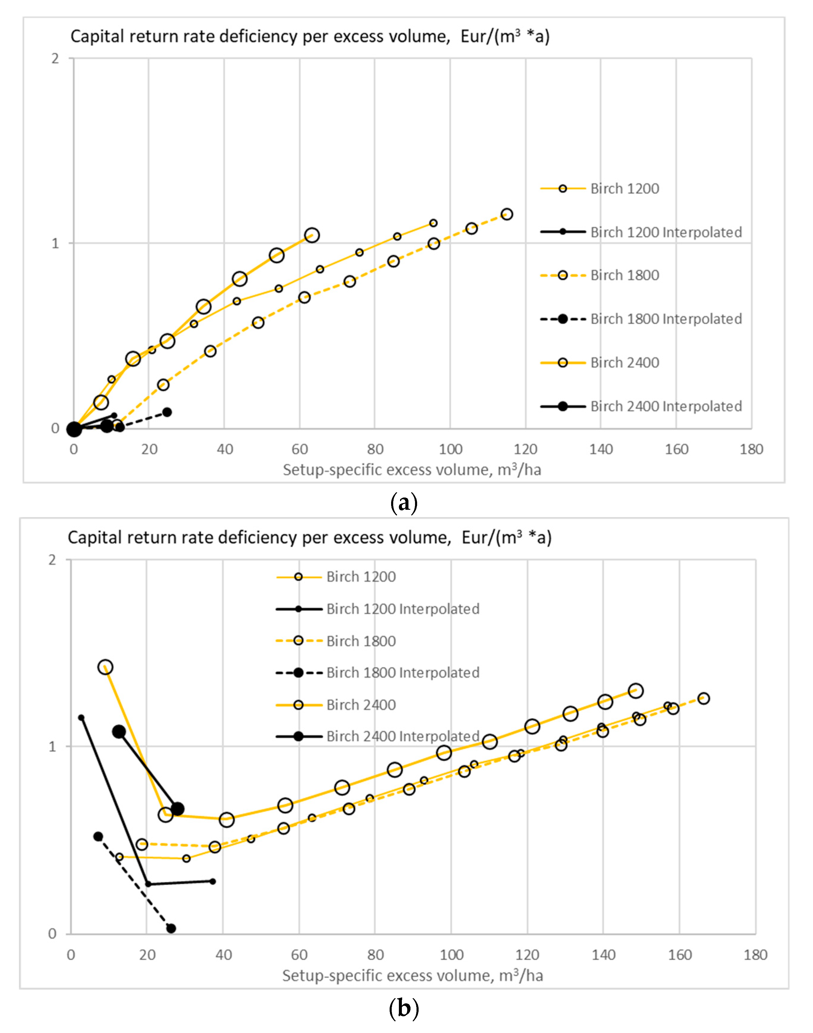
Figure 12, Figure 13 and Figure 14 show the expected value of the capital return rate deficiency per excess volume unit as a function of excess volume, within stands of three tree species where the growth model is applied as early as applicable, in the presence of eventual thinning restrictions. Thinning restrictions reduce the deficiency and increase available excess volume. Thinnings restricted to trees larger than 237 mm diameter show the smallest deficiency with moderate excess volume, while the omission of thinnings shows the smallest deficiency at large excess volumes. Application of Equation (8) in the determination of capitalization, instead of Equation (10), produces only small values of excess volume. Again, large excess volumes are not achievable using the interpolation Formula (8) since the internal consistency condition (12) becomes violated with increasing rotation age.
4. Discussion
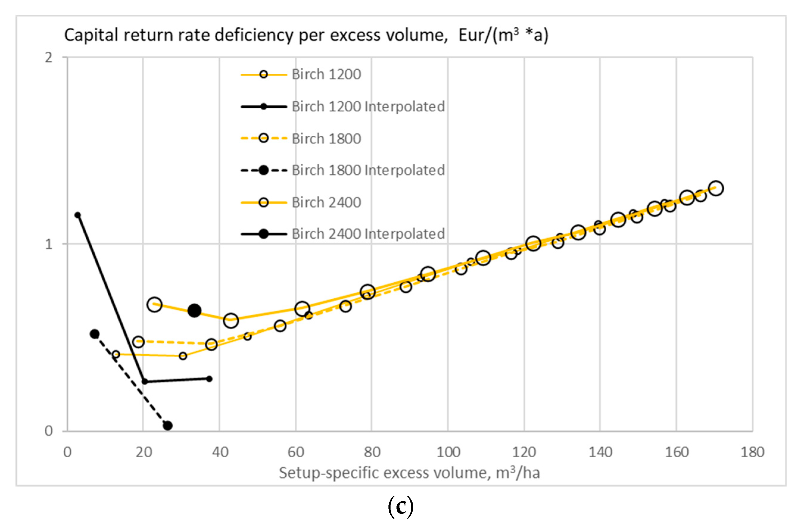
Interestingly, along with increasing rotation age, any application of Equation (8) presented in this paper terminates in violation of the internal consistency condition (12). This raises a doubt whether Equation (8) possibly induces some bias even in the circumstances where the consistency condition (12) is not violated. This is discussed in Figure 15, where a spruce stand of initial sapling density 1800/ha is grown to 109 years using Equation (10), and snapshots with Equation (8) are taken at 74 and 109 years of rotation. At 74 years of rotation, the exponential interpolation by Equation (8) appears to operate nicely. The estimate of the expected value of capitalization using Equation (8) is greater than that resulting from Equation (10), and one can reasonably assume the difference corresponding to a capitalization premium based on expected further value increment of young stands.
However, at the age of 109 years, the growth according to Equation (10) significantly differs from exponential, and the exponential interpolation clearly produces a bias. In fact, the estimate of the expected value of capitalization using Equation (8) is smaller than that resulting from Equation (10). One can reasonably suspect that any estimate produced using Equation (8) is reduced in comparison to Equation (10) along with increasing rotation age, even if the consistency condition (12) would not be strictly violated. This indicates that the longer rotation ages due to the application of Equation (8) in Figure 1, Figure 2, Figure 3, Figure 4, Figure 5, Figure 6, Figure 7, Figure 8, Figure 9 and Figure 10 possibly are not real, but maybe computational artifacts. Correspondingly, the capital return rate deficiencies produced with Equation (8) in Figure 11, Figure 12, Figure 13 and Figure 14 possibly shall not be trusted. It appears that the intangible young stand expectation premium cannot be produced in terms of exponential interpolation over the rotation age.
As the determination of the intangible capitalization appears unsuccessful, it is worth discussing the above results omitting the intangible premium. The two independent sets of initial conditions appear to yield similar results. The capital return rate is a weak function of rotation age, which results in variability in the optimal number of thinnings (Figure 1, Figure 2, Figure 3, Figure 4 and Figure 5). Restricting thinnings increases timber stock but reduces rotation age (Figure 6, Figure 7, Figure 8, Figure 9 and Figure 10). Increased timber stock induces a capital return rate deficiency (Figure 11, Figure 12, Figure 13 and Figure 14). The deficiency per excess volume unit is smaller if the severity of any thinning is restricted, in comparison to extending rotations (Figure 11, Figure 12, Figure 13 and Figure 14). Moderate increases in timber stock can be gained by restricting thinnings to large trees, while large increases are best achieved by omitting thinnings (Figure 11, Figure 12, Figure 13 and Figure 14).
The two datasets used this study relate differently concerning the intangible premium. The absence of the premium is an obvious deficiency in the first dataset. The second dataset however describes stand development through exponential interpolation up to the time of observation of wooded stands. Robustness of the findings is indicated since the two different datasets agree in the main findings.
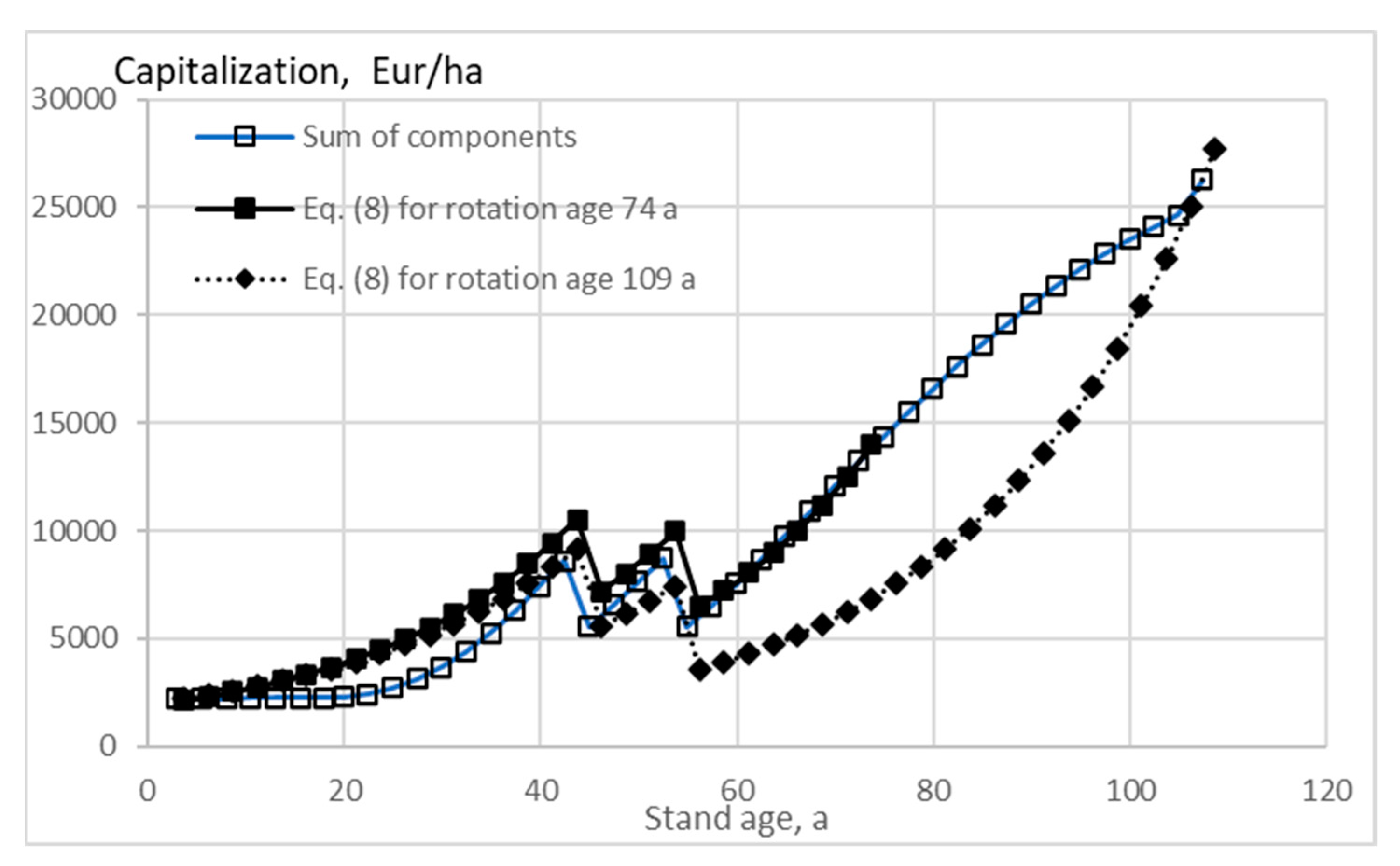
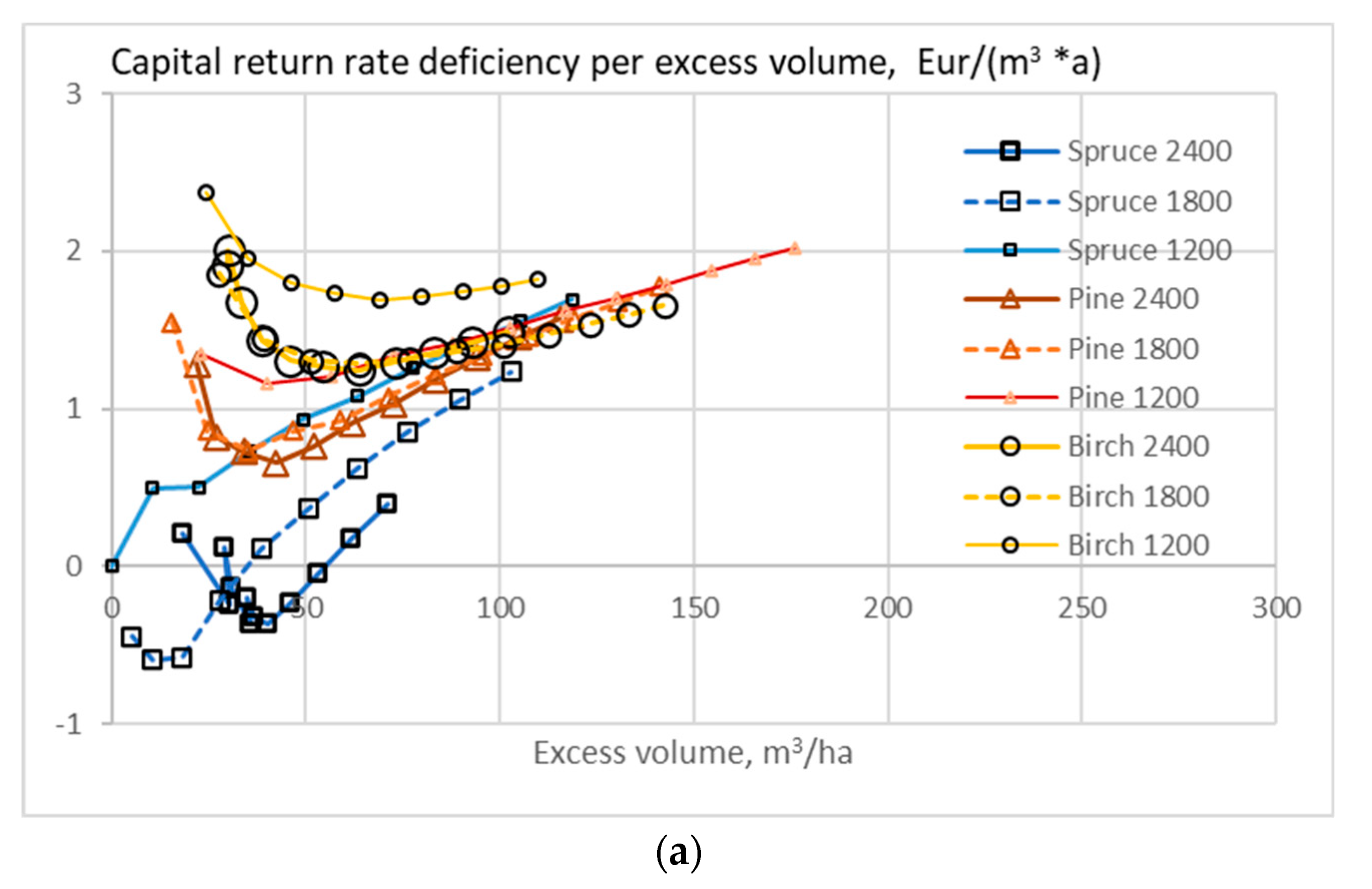
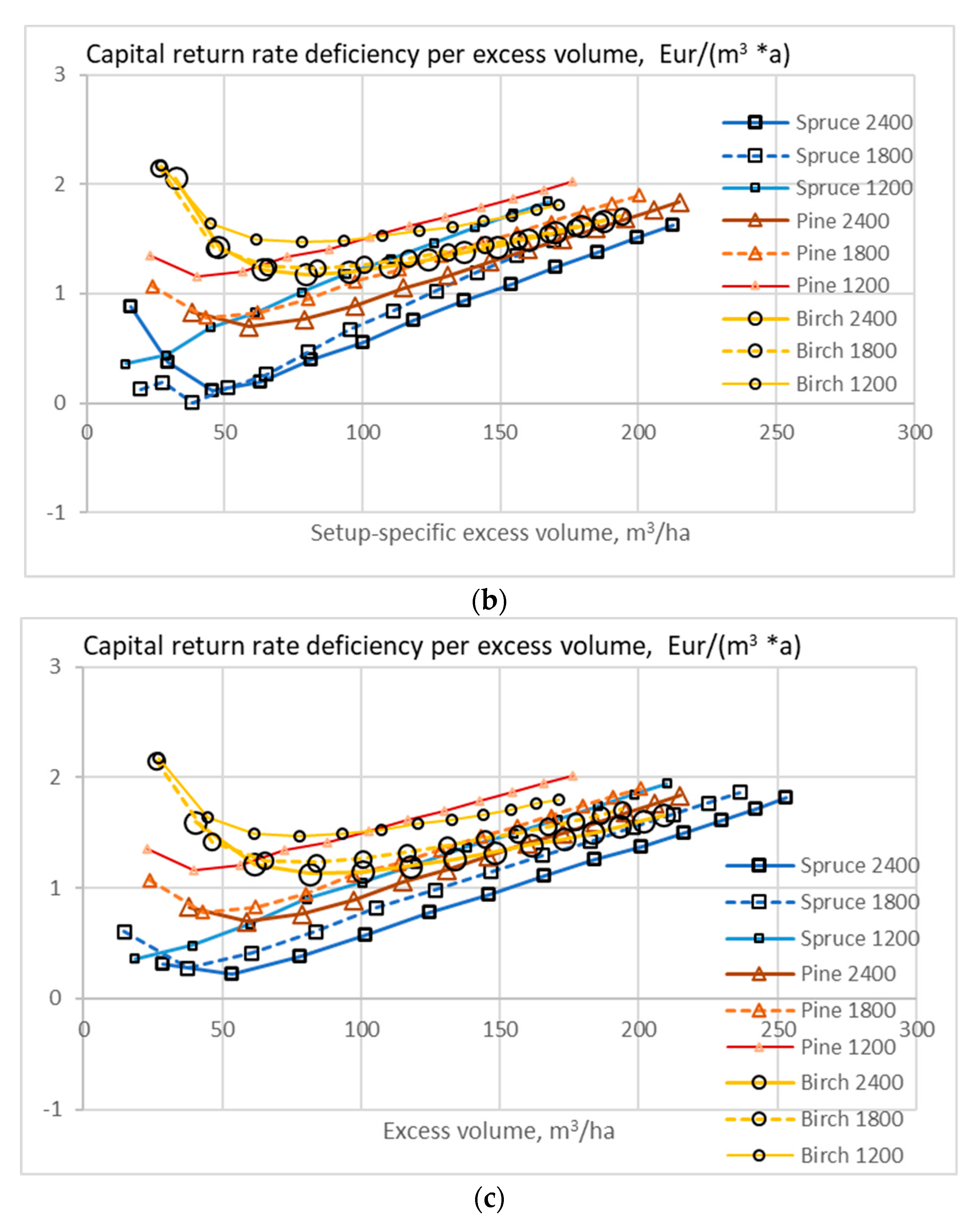
When the growth model has been applied on growing stands as early as applicable, control parameters have included not only thinning restrictions but also the selection of tree species, as well as initial sapling densities. The capital return rate deficiencies plotted in Figure 12, Figure 13 and Figure 14, however, are case-specific: any tree species and sapling density are taken as reference points of their own. It is possible to replot these Figures with one common reference. Here, we select spruce stands with sapling density 1200/ha as a common reference. The reason for this is that the capital return rate achievable according to Figure 4 is only slightly less than with spruce stands with greater sapling densities, but the duration risk is much less [45,46,47].
We find from Figure 16 that a small excess volume can inexpensively be gained by increasing sapling density. Greater excess volume is best achieved by restricting thinnings. A large excess volume is best achieved by omitting thinnings.
Figure 16 indicates that a significant excess volume can be produced at the expense of a monetary capital return rate deficiency in the order of one to two Euros/excess cubic meter per annum. This can be easily compensated by a carbon rent derived from European carbon emission prices valid at the time of writing [18,19,40]. On the other hand, such compensation is needed to achieve a large-scale increment in carbon sequestration. It has been recently shown that the carbon stock can be increased without deteriorating the wood supply for forest-based industries [40].
It is worth noting that this paper focusing on capitalization and capital return rate in terms of timber stock, the results apply to productive boreal forests, mostly on mineral soil. Another issue is that the only intangible asset discussed has been the growth expectation premium. It appears that the real estate market has recently gained momentum in terms of a goodwill value. The effect of inflated capitalizations on carbon economics shall be investigated in a forthcoming study.
5. Conclusions
It appears that the intangible young stand expectation premium cannot be produced in terms of exponential interpolation over the rotation age. It is worth discussing the results omitting the intangible premium. The capital return rate is a weak function of rotation age. Restricting thinnings increases timber stock but reduces rotation age. A small excess volume can inexpensively be gained by increasing sapling density. Greater excess volume is best achieved by restricting thinnings. A large excess volume is best achieved by omitting thinnings. Increased timber stock induces a capital return rate deficiency. This can be easily compensated by a carbon rent derived from European carbon emission prices valid at the time of writing.
Funding
This work was partially funded by Niemi foundation, grant III. The funder had no role in study design, data collection and analysis, decision to publish, or preparation of the manuscript.
Data Availability Statement
This paper has used raw data made available in referenced earlier papers.
Acknowledgments
Lauri Mehtätalo is gratefully acknowledged for fruitful discussions.
Conflicts of Interest
The author declares no conflict of interest. The funders had no role in the design of the study; in the collection, analyses, or interpretation of data; in the writing of the manuscript; or in the decision to publish the results.
References
- The Ocean, a Carbon Sink. Available online: https://ocean-climate.org/en/awareness/the-ocean-a-carbon-sink/ (accessed on 17 July 2021).
- Hauck, J.; Zeising, M.; Le Quéré, C.; Gruber, N.; Bakker, D.C.E.; Bopp, L.; Chau, T.T.T.; Gürses, Ö.; Ilyina, T.; Landschützer, P.; et al. Consistency and Challenges in the Ocean Carbon Sink Estimate for the Global Carbon Budget. Front. Mar. Sci. 2020, 7, 852. [Google Scholar] [CrossRef]
- Friedel, M. Forests as Carbon Sinks. Available online: https://www.americanforests.org/blog/forests-carbon-sinks/ (accessed on 17 July 2021).
- Goodale, C.L.; Apps, M.J.; Birdsey, R.A.; Field, C.B.; Heath, L.S.; Houghton, R.A.; Jenkins, J.C.; Kohlmaier, G.H.; Kurz, W.; Liu, S.; et al. Forest carbon sinks in the northern hemisphere. Ecol. Appl. 2002, 12, 891–899. [Google Scholar] [CrossRef]
- Adams, A.; Harrison, R.; Sletten, R.; Strahm, B.; Turnblom, E.; Jensen, C. Nitrogen-fertilization impacts on carbon sequestration and flux in managed coastal Douglas-fir stands of the Pacific Northwest. For. Ecol. Manag. 2005, 220, 313–325. [Google Scholar] [CrossRef]
- Lal, R. Forest soils and carbon sequestration. For. Ecol. Manag. 2005, 220, 242–258. [Google Scholar] [CrossRef]
- Liski, J.; Lehtonen, A.; Palosuo, T.; Peltoniemi, M.; Eggersa, T.; Muukkonen, P.; Mäkipää, R. Carbon accumulation in Finland’s forests 1922-2004-an estimate obtained by combination of forest inventory data with modelling of biomass, litter and soil. Ann. For. Sci. 2006, 63, 687–697. [Google Scholar] [CrossRef]
- Peltoniemi, M.; Mäkipää, R.; Liski, J.; Tamminen, P. Changes in soil carbon with stand age—An evaluation of a modelling method with empirical data. Glob. Chang. Biol. 2004, 10, 2078–2091. [Google Scholar] [CrossRef]
- Powers, M.; Kolka, R.; Palik, B.J.; McDonald, R.; Jurgensen, M. Long-term management impacts on carbon storage in Lake States forests. For. Ecol. Manag. 2011, 262, 424–431. [Google Scholar] [CrossRef]
- Riikilä, M. Avohakkuu ei Hävitä Hiilivarastoa. Metsälehti 21/2020. Available online: https://www.metsalehti.fi/artikkelit/avohakkuu-ei-havita-hiilivarastoa/#928d2873 (accessed on 17 July 2021).
- Campioli, M.; Vicca, S.; Luyssaert, S.; Bilcke, J.; Ceschia, E.; Iii, F.S.C.; Ciais, P.; Fernández-Martínez, M.; Malhi, Y.; Obersteiner, M.; et al. Biomass production efficiency controlled by management in temperate and boreal ecosystems. Nat. Geosci. 2015, 8, 843–846. [Google Scholar] [CrossRef]
- Thornley, J.H.M.; Cannell, M.G.R. Managing forests for wood yield and carbon storage: A theoretical study. Tree Physiol. 2000, 20, 477–484. [Google Scholar] [CrossRef]
- Weisstein, E. Chaos. Wolfram Web Resources. Available online: https://mathworld.wolfram.com/Chaos.html (accessed on 17 July 2021).
- Kärenlampi, P.P. Diversity of Carbon Storage Economics in Fertile Boreal Spruce (Picea Abies) Estates. Sustainability 2021, 13, 560. [Google Scholar] [CrossRef]
- Kärenlampi, P.P. Capital return rate and carbon storage on forest estates of three boreal tree species. Sustainability 2021, 13, 6675. [Google Scholar] [CrossRef]
- Kärenlampi, P.P. State-space approach to capital return in nonlinear growth processes. Agric. Finance Rev. 2019, 79, 508–518. [Google Scholar] [CrossRef] [Green Version]
- Kärenlampi, P.P. Estate-Level Economics of Carbon Storage and Sequestration. Forests 2020, 11, 643. [Google Scholar] [CrossRef]
- Kärenlampi, P.P. The Effect of Empirical Log Yield Observations on Carbon Storage Economics. Forests 2020, 11, 1312. [Google Scholar] [CrossRef]
- Lintunen, J.; Laturi, J.; Uusivuori, J. How should a forest carbon rent policy be implemented? For. Policy Econ. 2016, 69, 31–39. [Google Scholar] [CrossRef]
- Kilkki, P.; Väisänen, U. Determination of the optimum cutting policy for the forest stand by means of dynamic programming. Acta For. Fenn. 1969, 102, 1–29. [Google Scholar] [CrossRef]
- Haight, R.G.; Monserud, R.A. Optimizing any-aged management of mixed-species stands. II: Effects of decision criteria. For. Sci. 1990, 36, 125–144. [Google Scholar]
- Pukkala, T.; Lähde, E.; Laiho, O. Optimizing the structure and management of uneven-sized stands in Finland. Forestry 2010, 83, 129–142. [Google Scholar] [CrossRef]
- Tahvonen, O. Optimal structure and development of uneven-aged Norway spruce forests. Can. J. For. Res. 2011, 41, 2389–2402. [Google Scholar] [CrossRef]
- Rosa, R.; Soares, P.; Tomé, M. Evaluating the Economic Potential of Uneven-aged Maritime Pine Forests. Ecol. Econ. 2018, 143, 210–217. [Google Scholar] [CrossRef]
- Tahvonen, O. Economics of rotation and thinning revisited: The optimality of clearcuts versus continuous cover forestry. For. Policy Econ. 2016, 62, 88–94. [Google Scholar] [CrossRef]
- Pukkala, T. Instructions for optimal any-aged forestry. For. Int. J. For. Res. 2018, 91, 563–574. [Google Scholar] [CrossRef]
- Tahvonen, O.; Pukkala, T.; Laiho, O.; Lähde, E.; Niinimäki, S. Optimal management of uneven-aged Norway spruce stands. For. Ecol. Manag. 2010, 260, 106–115. [Google Scholar] [CrossRef]
- Jin, X.; Pukkala, T.; Li, F. A new approach to the development of management instructions for tree plantations. For. Int. J. For. Res. 2019, 92, 196–205. [Google Scholar] [CrossRef]
- Buongiorno, J.; Halvorsen, E.A.; Bollandsås, O.M.; Gobakken, T.; Hofstad, O. Optimizing management regimes for carbon storage and other benefits in uneven-aged stands dominated by Norway spruce, with a derivation of economic supply of carbon storage. Scand. J. For. Res. 2012, 27, 460–473. [Google Scholar] [CrossRef]
- Tahvonen, O.; Rautiainen, A. Economics of forest carbon storage and the Additionality principle. Resour. Energy Econ. 2017, 50, 124–134. [Google Scholar] [CrossRef] [Green Version]
- Assmuth, A.; Rämö, J.; Tahvonen, O. Optimal Carbon Storage in Mixed-Species Size-Structured Forests. Environ. Resour. Econ. 2021, 79, 249–275. [Google Scholar] [CrossRef]
- Rämö, J.; Tahvonen, O. Economics of harvesting boreal uneven-aged mixed-species forests. Can. J. For. Res. 2015, 45, 1102–1112. [Google Scholar] [CrossRef]
- Parkatti, V.-P.; Assmuth, A.; Rämö, J.; Tahvonen, O. Economics of boreal conifer species in continuous cover and rotation forestry. For. Policy Econ. 2019, 100, 55–67. [Google Scholar] [CrossRef]
- Sinha, A.; Rämö, J.; Malo, P.; Kallio, M.; Tahvonen, O. Optimal management of naturally regenerating uneven-aged forests. Eur. J. Oper. Res. 2017, 256, 886–900. [Google Scholar] [CrossRef] [Green Version]
- Parkatti, V.-P.; Tahvonen, O. Optimizing continuous cover and rotation forestry in mixed-species boreal forests. Can. J. For. Res. 2020, 50, 1138–1151. [Google Scholar] [CrossRef]
- Speidel, G. Forstliche Betreibswirtschaftslehre, 2nd ed.; Verlag Paul Parey: Hamburg, Germany, 1967; p. 226. (in German) [Google Scholar]
- Speidel, G. Planung in Forstbetrieb, 2nd ed.; Verlag Paul Parey: Hamburg, Germany, 1972; p. 270. (in German) [Google Scholar]
- Kärenlampi, P.P. Harvesting Design by Capital Return. Forests 2019, 10, 283. [Google Scholar] [CrossRef] [Green Version]
- Leslie, A.J. A review of the concept of the normal forest. Aust. For. 1966, 30, 139–147. [Google Scholar] [CrossRef]
- Kärenlampi, P.P. Two Sets of Initial Conditions on Boreal Forest Carbon Storage Economics. Preprints 2021, 2021070439. [Google Scholar] [CrossRef]
- Tiwari, R. Intrinsic value estimates and its accuracy: Evidence from Indian manufacturing industry. Future Bus. J. 2016, 2, 138–151. [Google Scholar] [CrossRef] [Green Version]
- Tanjung, G. The applications of discount cash flow, abnormal earning, and relative valuation approach (Firm Intrinsic Value Analysis Pada Perusahaan BUMN). In Proceedings of the Seminar Nasional Kewirausahaan dan Inovasi Bisnis IVAt, Jakarta, Indonesia, 8 May 2014. [Google Scholar]
- Carlin, S. How To Calculate Intrinsic Value (Formula—Excel Template & AMZN Example). Available online: https://svencarlin.com/how-to-calculate-intrinsic-value-formula/ (accessed on 14 September 2021).
- Kärenlampi, P.P. Wealth accumulation in rotation forestry–Failure of the net present value optimization? PLoS ONE 2019, 14, e0222918. [Google Scholar] [CrossRef]
- Bouchaud, J.-P.; Potters, M. Théorie des Risques Financiers (Saclay: Aléa) 1997 (English translation 2000) Theory of Financial Risks (Cambridge: Cambridge University Press)). Available online: http://web.math.ku.dk/~rolf/Klaus/bouchaud-book.ps.pdf. (accessed on 25 December 2021).
- Brealey, R.A.; Myers, S.C.; Allen, F. Principles of Corporate Finance, 10th ed.; McGraw-Hill Irwin: New York, NY, USA, 2011. [Google Scholar]
- Fabozzi, F.J. Capital Markets: Institutions, Instruments, and Risk Management; MIT Press: Cambridge, MA, USA, 2015. [Google Scholar]
- Bollandsås, O.M.; Buongiorno, J.; Gobakken, T. Predicting the growth of stands of trees of mixed species and size: A matrix model for Norway. Scand. J. For. Res. 2008, 23, 167–178. [Google Scholar] [CrossRef]
Figure 1.
The expected value of capital return rate, as a function of rotation age, when the growth model is applied to four observed wooded stands, without any thinning restriction (a), good-quality trees of at least 238 mm of diameter only removed in thinning (b), and without any commercial thinning (c).

Figure 2.
The expected value of capital return rate, as a function of rotation age, when the growth model is applied to three observed wooded stands, without any thinning restriction (a), good-quality trees of at least 238 mm of diameter only removed in thinning (b), and without any commercial thinning (c).

Figure 3.
The expected value of capital return rate on pine (Pinus sylvestris) stands of different initial sapling densities, as a function of rotation age, when the growth model is applied as early as applicable, without any thinning restriction (a), good-quality trees of at least 238 mm of diameter only removed in thinning (b). Figure 3b does not contain any commercial thinning.

Figure 4.
The expected value of capital return rate on spruce stands of different initial sapling densities, as a function of rotation age, when the growth model is applied as early as applicable, without any thinning restriction (a), good-quality trees of at least 238 mm of diameter only removed in thinning (b), and without commercial thinning (c).

Figure 5.
The expected value of capital return rate on birch (Betula pendula) stands of different initial sapling densities, as a function of rotation age, when the growth model is applied as early as applicable, without any thinning restriction (a), good-quality trees of at least 238 mm of diameter only removed in thinning (b), and without commercial thinning (c).

Figure 6.
Stand capitalization as a function of stand age, when the growth model is applied to four observed wooded stands, without any thinning restriction (a), good-quality trees of at least 238 mm of diameter only removed in thinning (b), and without any commercial thinning (c).
Figure 6.
Stand capitalization as a function of stand age, when the growth model is applied to four observed wooded stands, without any thinning restriction (a), good-quality trees of at least 238 mm of diameter only removed in thinning (b), and without any commercial thinning (c).

Figure 7.
Stand capitalization as a function of stand age, when the growth model is applied to three observed wooded stands, without any thinning restriction (a), good-quality trees of at least 238 mm of diameter only removed in thinning (b), and without any commercial thinning (c).
Figure 7.
Stand capitalization as a function of stand age, when the growth model is applied to three observed wooded stands, without any thinning restriction (a), good-quality trees of at least 238 mm of diameter only removed in thinning (b), and without any commercial thinning (c).

Figure 8.
Capitalization on pine stands of different initial sapling densities, as a function of stand age, when the growth model is applied as early as applicable, without any thinning restriction (a), good-quality trees of at least 238 mm of diameter only removed in thinning (b). Figure 8b does not contain any commercial thinning.

Figure 9.
Capitalization on spruce stands of different initial sapling densities, as a function of stand age, when the growth model is applied as early as applicable, without any thinning restriction (a), good-quality trees of at least 238 mm of diameter only removed in thinning (b), and without any commercial thinning (c).

Figure 10.
Capitalization on birch stands of different initial sapling densities, as a function of stand age, when the growth model is applied as early as applicable, without any thinning restriction (a), good-quality trees of at least 238 mm of diameter only removed in thinning (b), and without any commercial thinning (c).

Figure 11.
The expected value of capital return rate deficiency per excess volume unit, as a function of excess volume, when the growth model is applied to seven observed wooded stands, without any thinning restriction (a), good-quality trees of at least 238 mm of diameter only removed in thinning (b), and without any commercial thinning (c).


Figure 12.
The expected value of capital return rate deficiency per excess volume unit on pine stands of different initial sapling densities, as a function of excess volume, when the growth model is applied as early as applicable, without any thinning restriction (a), good-quality trees of at least 238 mm of diameter only removed in thinning (b). Figure 12b does not contain any commercial thinning.


Figure 13.
The expected value of capital return rate deficiency per excess volume unit on spruce stands of different initial sapling densities, as a function of excess volume, when the growth model is applied as early as applicable, without any thinning restriction (a), good-quality trees of at least 238 mm of diameter only removed in thinning (b), and without any commercial thinning (c).


Figure 14.
The expected value of capital return rate deficiency per excess volume unit on birch stands of different initial sapling densities, as a function of excess volume, when the growth model is applied as early as applicable, without any thinning restriction (a), good-quality trees of at least 238 mm of diameter only removed in thinning (b), and without any commercial thinning (c).


Figure 15.
Capitalization of a spruce stand established with 1800 saplings as a function of stand age, according to Equation (10), and with two snapshots according to Equation (8).
Figure 15.
Capitalization of a spruce stand established with 1800 saplings as a function of stand age, according to Equation (10), and with two snapshots according to Equation (8).

Figure 16.
The expected value of capital return rate deficiency per excess volume unit on stands of different initial sapling densities, as a function of excess volume when the growth model is applied as early as applicable, without any thinning restriction (a), good-quality trees of at least 238 mm of diameter only removed in thinning (b), and without any commercial thinning (c). The expected value of capital return rate and stand volume from spruce stands with 1200 seedlings per hectare are taken as a common reference.


Publisher’s Note: MDPI stays neutral with regard to jurisdictional claims in published maps and institutional affiliations. |
© 2022 by the author. Licensee MDPI, Basel, Switzerland. This article is an open access article distributed under the terms and conditions of the Creative Commons Attribution (CC BY) license (https://creativecommons.org/licenses/by/4.0/).
Share and Cite
MDPI and ACS Style
Kärenlampi, P.P. Capitalization and Capital Return in Boreal Carbon Forestry. Earth 2022, 3, 204-227. https://0-doi-org.brum.beds.ac.uk/10.3390/earth3010014
AMA Style
Kärenlampi PP. Capitalization and Capital Return in Boreal Carbon Forestry. Earth. 2022; 3(1):204-227. https://0-doi-org.brum.beds.ac.uk/10.3390/earth3010014
Chicago/Turabian StyleKärenlampi, Petri P. 2022. "Capitalization and Capital Return in Boreal Carbon Forestry" Earth 3, no. 1: 204-227. https://0-doi-org.brum.beds.ac.uk/10.3390/earth3010014