Development of a Line Source Dispersion Model for Gaseous Pollutants by Incorporating Wind Shear near the Ground under Stable Atmospheric Conditions ^†

Abstract

Transportation sources are a major contributor to air pollution in urban areas. The role of air quality modeling is vital in the formulation of air pollution control and management strategies. Many models have appeared in the literature to estimate near-field ground level concentrations from mobile sources moving on a highway. However, current models do not account explicitly for the effect of wind shear (magnitude) near the ground while computing the ground level concentrations near highways from mobile sources. This study presents an analytical model based on the solution of the convective-diffusion equation by incorporating the wind shear near the ground for gaseous pollutants. The model input includes emission rate, wind speed, wind direction, turbulence, and terrain features. The dispersion coefficients are based on the near field parameterization. The sensitivity of the model to compute ground level concentrations for different inputs is presented for three different downwind distances. In general, the model shows Type III sensitivity (i.e., the errors in the input will show a corresponding change in the computed ground level concentrations) for most of the input variables. However, the model equations should be re-examined for three input variables (wind velocity at the reference height and two variables related to the vertical spread of the plume) to make sure that that the model is valid for computing ground level concentrations.

1. Introduction

Air pollution can be either from natural sources or man-made sources. Combustion of fossil, biomass, and other non-renewable fuels is the primary contributor to man-made emissions we face today [1]. More than 55% of people in the world are currently living in urban areas, and 68% are projected to live in urban areas by 2050 [2]. Transportation sources such as cars and trucks are extensively used in urban areas to carry out day to day living. Air pollution caused by transportation sources contributes to smog and poor air quality, which have negative impacts on public health [3]. The air pollution impact of transportation sources is studied using either dispersion models or field studies. Air quality modeling helps to establish a relation between the pollution sources and their impacts. The mathematical techniques are used to simulate ground-level concentrations in air quality models. Inputs of air quality modeling include meteorological data, source information, and surrounding terrain [4].

The air quality models are developed to predict the concentrations of current and future situations. Most of the models are developed using the standard input parameters and evaluated with the real-time experimental data. The main aim of these models is to provide suggestions and ideas about the future air quality condition for the policymakers to make regulatory decisions to protect public health [5]. There are different types of models based on sources (such as point, line, and area sources). Line sources are the models used to calculate and predict the concentration of pollutants that are continuously emitted from the automobiles on highways. The effect of pollution from line sources is high in an urban environment due to their major contribution. Vehicular density, vehicle speed, and emission rate are the major variable to be considered for the prediction analysis of air quality involving mobile sources [6,7,8]. The air quality models, in general, are divided based on attributes and model category, as mentioned in

Table 1. The major classification of air quality models based on different model categories [7].

Attributes	Model Category
Source	Point, line, area, volume, flare
Receptor	Street Canyon, intersection model
Frame	Lagrangian, Eulerian
Dimensionality	Single, double, triple, or multidimensional
Scale	Microscale and mesoscale, small synoptic, large synoptic, planetary
Structure	Analytical, statistical
Approach	Numerical, experimental
Applicability	Simple terrain, complex terrain, rural flat terrain, urban flat terrain, coastal terrain
Complexity	Screen models, refined models

.

2. Literature Review

The literature review indicates that many line source air quality models have been developed over the last 50 years. The mathematical formulation of these models is analytical, statistical, or numerical. The solution of the convective-diffusion equation for a line source was available in the 1950s [9]. During the 1960s and 1970s, many Gaussian-based dispersion models were introduced. These formulations were a function of meteorology, receptor locations, and highway geometry. The differences in formulations were due to the assumption made during the solution of the convective-diffusion equation or the specification of plume spread rates. However, these models did not perform very well when the predicted results were compared with the observed values. The primary reason was difficulty in accounting for atmospheric dispersion and turbulence [10]. Subsequently, many experimental field studies were conducted to improve the models.

HIWAY1 was developed in the early 1970s to predict mobile source emissions near roadways [11]. In 1978, Chock formulated the GM line source model by incorporating wind speed correction and modified values for vertical dispersion coefficients to address wake turbulence from the vehicles [12]. In 1980, Rao and Keenan evaluated the existing models and suggested new dispersion curves for pollution dispersion near highways [13,14]. Model development continued from the 1980s onward to address vehicle induced turbulence, surface roughness, averaging time, new provisions for plume spread, and other turbulence mixing parameters [15].

United States Environmental Protection Agency (USEPA) Office of Research and Development introduced a California Line Source (CALINE) model in 1972 based on the Gaussian plume model using Pasquill–Gifford atmospheric stability classes. CALINE was developed by focusing on the prediction of CO concentration near roadways [16]. In 1975, formulations for depressed roadways were added to develop CALINE2 [17]. In 1979, the vertical and horizontal dispersion curves were updated along with updating vehicle-induced turbulence, averaging time, and introducing a finite line source to develop CALINE3 to reduce over predictions. In 1984, CALINE4 was introduced with the addition of chemistry for NO₂ and PM, intersections, and updating lateral plume spread and vehicle induced turbulence. CALINE, CALINE2, and CALINE3 are open-source models and are available freely to the public, unlike CALINE4 [18]. Around the early 1990s, CAL3QHC screening model was developed to auto-estimate the queue lengths of vehicles at the intersections. The enhanced version of CAL3QHC is CAL3QHR, a more flexible model than CAL3QHC with a two-tiered approach [19]. In the same decade, Industrial Source Complex Short Term 2 (ISCST2) was introduced by the incorporation of mixing height algorithms. It could estimate the concentration of pollutants with varying emissions from point sources. ISCST3 was developed in 1995 by incorporating the new area source option and algorithms of dry deposition [20]. A commonly used line source model CALINE4 uses a range of traffic and fleet characteristics and a diffusion equation to assess the impacts of a road at a small scale. It is specifically designed for assessing air quality impacts at roadways or intersections and used to predict impacts of changing traffic volumes, signal phasing, or adding additional lanes to a roadway [21]. In New Zealand, a similar model, named VEPM, was developed, which used real and lab-based emissions data to predict emissions up to the year 2040 from a roadway [22].

In 1989, Luhar and Patil developed the general finite line source model (GFLSM) based on the Gaussian diffusion equation and evaluated based on data collected at intersections in, Mumbai and New York [23]. Later the GFLSM was improved by Sharma (1999) based on experiments conducted at intersections in Delhi, India [24]. According to Eerens, the CAR model was developed in 1993 and evaluated with the data collected in urban areas of the Netherlands [25]. A road network dispersion model named CAR-FMI was developed like a CAR model to predict concentrations of pollutants from automobiles near industrial areas [26]. ROADWAY model was developed while studying the vehicle wakes and the dispersion phenomena in pollutants from the vehicles [27]. COPERT and CEM are also other major models used to calculate the concentration of pollutants from vehicular emissions [28].

The research has continued to develop, assess, and evaluate the pre-existing models and increase the scope of accuracy for future models. In 2002, Christoffer mentioned that the spread of the pollutant dispersion about the center of mass is non-spherical under shear conditions, and the pollution shape reflects the vertical wind shear profile experienced by the puff within 4 h of the time scale for the point releases [29]. In 2007, Gokhale developed a simple semi-empirical box model based on the “traffic flow rate” at the busiest traffic road intersections in Delhi. He estimated hourly average carbon monoxide (CO) concentrations and optimized specific vehicle emission rates based on vehicle category. Through this study, he was able to show that the nature of the vehicle flows influences the rate and nature of the dispersion of pollutants which influence pollutant concentration in the road vicinity [30]. In 2018, Milando conducted a study near high traffic roads in Detroit. He evaluated the RLINE by comparing predicted concentrations of NO_x, CO, and PM_2.5. The model performance for CO and NO_x was found to be best at sites close to major roads, during downwind conditions, during weekdays, and in certain seasons [31]. In 2018, Bowatte investigated longer-term effects of traffic-related air pollution exposure for individuals with or without existing asthma, and with or without lower lung function. For middle-aged adults, living less than 200 m from a major road influences both the development and persistence of asthma. These findings have public health implications for asthma prevention strategies in primary and secondary settings [32]. In 2011 Xie conducted a research study on both the daily and hourly concentration levels of CO, PM₁₀, NO₂, and O₃ during the Beijing Olympic Games and conformed to the Grade II China national ambient air quality standards. A notable reduction of concentration levels was observed in different regions of Beijing, with the traffic-related air pollution in the downwind northern and western areas. According to Xie, “TRS policy was therefore effective in alleviating traffic-related air pollution and improving short-term air quality during the Beijing Olympic Games” [33]. In 2018, Liang conducted a dorm room inhalation study due to vehicle emissions, using a near-road monitor as a surrogate for true exposure, and observed acute health effects. This study was conducted near-road measurements of several single traffic indicators at six indoor and outdoor sites [34]. Later in 2020, Amoatey made a comparative study between COPERT and CEM models. The correlation coefficient for these two models was found to be statistically significant from 0 in the case of combined model comparison across all the traffic locations for both CO and NO_x. He concluded that, due to the terrain features of certain roads, weak performance is observed and needs to be considered in future study [35].

In 2005, the USEPA replaced the ISC model with AERMOD, which contains an updated atmospheric stability scheme and the ability to characterize the planetary boundary layer through both surface and mixed layers. The latest line source model RLINE is being incorporated in AERMOD by the USEPA [36]. Some of the popular air quality models related to transportation sources and their key features are mentioned in

Table 2. Various popular air quality models and some of their key features.

Model	Some Key Features
GFLSM	◦ Better performance with a finite length line source. ◦ Any orientation of wind direction with roadways can be used. ◦ No constraint on infinite line source. ◦ Used for both gaseous pollutants and particulate matter. ◦ Effectively predicts the pollutant concentration near intersections.
CAL3QHR	◦ Allowed for refined analyses. ◦ Processes up to a week of hourly data from the input file. ◦ Used in both rural and urban conditions. ◦ Calculates the nine highest 8-h running average concentrations for each receptor.
COPERT	◦ National, regional, or local scale emissions are computed. especially when a particular vehicle type is “artificially” promoted or discouraged from circulation. ◦ Includes all main pollutants (e.g., greenhouse gases, air pollutants, and toxic species). ◦ All relevant road vehicle operation mode emissions are estimated. ◦ Choice of the calculation method. ◦ Non-exhaust emissions, such as fuel evaporation from vehicles, are not included.
CALINE4	◦ Can predict concentrations of pollutants for receptors within 500 m of the roadway and includes a mixing zone concept. ◦ Special options for intersections, street canyons, and parking facilities are available. ◦ Can predict gaseous pollutants and suspended pollutants as well. ◦ More flexibility in terms of input parameter complexity. ◦ Easy to implement the model and various options for additional input parameters.
AERMOD	◦ Use stack tip downwash, gradual plume rise, buoyancy-induced dispersion, and calms-processing routines. ◦ Calculate wind profiles and vertical potential temperature gradients. ◦ Incorporated line source modeling option.

.

The literature review indicates that available line source dispersion models do not account for wind shear near the ground explicitly under different atmospheric conditions. Therefore, this study is focused on developing a line source dispersion model considering the wind shear near the ground under stable conditions. The model is applied to gaseous pollutants released from mobile sources on a highway. This paper presents a line source model (SLINE) by incorporating wind shear near the ground surface to predict the impact of mobile sources moving on a highway in nearby areas during stable atmospheric conditions. The sensitivity analysis is performed by considering the selected variables in the model which have an impact on the computed concentrations.

3. SLINE Model Development

The basic approach to develop this model was the incorporation of wind shear during the dispersion from a line source using the convective-diffusion equation. It is important to consider the variation of the wind velocity magnitude near the ground for the dispersion of pollutants released from the tailpipe of mobile sources. This physical phenomenon was incorporated in the derivation of the dispersion and transport equation for the SLINE model. The model was based on the analytical solution of the convective-diffusion equation of a line source given in the book by Sutton [9]. The assumptions used in deriving the equation were: (i) the wind direction is always perpendicular to the highway, (ii) the dispersion is of the non-fumigation type, (iii) the velocity profile with height above the ground level is assumed to be the same for all downwind distances, (iv) a power-law profile is assumed for the velocity, i.e., the magnitude of the wind velocity near the ground level changes rapidly and follows a power law, and (v) the eddy diffusivity profile is a conjugate of velocity profile as given in Equation (3) below.

3.1. Dispersion Model

The analytical solution of the convective-diffusion equation to calculate the concentration of pollutants at any downwind distance is given by Equation (1):

$$C_{\left(x,z\right)}=\frac{q}{u_1\ast \gamma \left(s\right)}\ast {[\frac{u_1}{{\left(m-n+2\right)}^2\ast K_1\ast x}]}^s\ast exp\left[-u_1\ast \frac{z^{m-n+2}}{({\left(m-n+2\right)}^2\ast K_1\ast x)}\right]$$

(1)

where C is the concentration of pollutants at a point; (x, z), x is the downwind distance; z is the vertical height of the receptor above the ground; q is the emission rate of the mobile source per unit length; m and n are the exponents of power-law velocity profile and eddy diffusivity profile, respectively; s is the stability parameter based on m and n; $u_1$ and $K_1$ are the wind velocity and eddy diffusivity at a reference height $z_1$, respectively, (see Equations (2) and (3)); $\mathrm{and} \gamma \left(s\right)$ is the gamma function of s.

The velocity and eddy diffusivity profiles are:

$$u=u_1\ast {(\frac{z}{z_1})}^m$$

(2)

$$K=K_1\ast {(\frac{z}{z_1})}^n$$

(3)

The value of $u_1$ is based on the measurement and $K_1$ is computed using the Equation (4) used by Rao et al. [37]; Nimmatoori and Kumar et al. [38].

$$K=\left(\frac{{\sigma }_z^2 u}{2x}\right)$$

(4)

The Equations (3) and (4) indicate that K, as well as $K_1$, is a function of downwind distance x. However, the derivation of Equation (1) assumes that K is constant as the plume moves downwind. It is assumed during the application of Equation (1) that the concentration is predicted in the SLINE model at a downwind distance by updating the value of $K_1$ in the model for that downwind distance. It is expected that this approach will improve the model performance.

3.2. Turbulence Parametrization

The vertical spread for stable conditions for low-level sources is based on theoretical considerations and experimental data and is given by Snyder et al [39] as Equation (5).

$${\sigma }_z=a\ast \frac{x u_{*}}{U_e}\ast \frac{1}{\left(1+b_s \frac{u_{*}}{U_e}{\left(\frac{x}{L}\right)}^{\frac{2}{3}}\right)}$$

(5)

where $U_e$ is the effective wind velocity, $u_{* }$ is the surface friction velocity, $\mathrm{and} L$ is the Monin–Obukhov length. The formulation for $U_{\overline{z}}, U_e, {\sigma }_v$, and $\overline{z}$ are provided in Equations (2) and (6)–(8), respectively. Equations (6)–(8) are from Snyder et al. [39]. The values for a and bs are 0.3 and 3, taken from Snyder’s RLINE formulation [39].

$$U_e=\sqrt{2{\sigma }_v{}^2+U_{\overline{\left(z\right)}}^2}$$

(6)

$${\sigma }_v=\sqrt{{\left(0.6w_{*}\right)}^2+{\left(1.9u_{*}\right)}^2}$$

(7)

$$\overline{z}={\sigma }_z\sqrt{\frac{2}{\pi }}exp[-\frac{1}{2}\left(\frac{z_s}{{\sigma }_z}{)}^2\right]+z_{s}erf\left(\frac{z_s}{\sqrt{2}{\sigma }_z}\right)$$

(8)

$U_{\overline{z}}$ velocity is the wind velocity at the reference height $\overline{z}$ and $z_s$ is the height from the ground surface to the tailpipe (emission source) of the mobile source.

However, the vertical spread in the current model incorporates the additional spread ($m_t$) due to the turbulence created by moving vehicles. Then, the modified equation used to calculate ${\sigma }_z$ is given in Equation (9).

$${\sigma }_z=\frac{a u_{*}x}{U_e\ast \left(1+b_s \frac{u_{*}}{U_e}{\left(\frac{x}{L}\right)}^{\frac{2}{3}}\right)}+m_t$$

(9)

$m_t$ is assumed equal to 50% of the effective height of mobile sources on the highway.

$\mathrm{For}\mathrm{the}\mathrm{current}\mathrm{model} {\sigma }_v=1.9u_{*}$ because the convective velocity scale $w_{*}$ for stable conditions is approximately 0 since the heat flux is either very small or zero. An expression of $K_1$ obtained as follows by substituting Equation (9) in Equation (4) with the help of Equation (3):

$$K_1=\frac{{\sigma }_z^2 u_1}{2x}={\left[\frac{a u_{*} x}{u_1+b_s{u}_{*}{\left(\frac{x}{L}\right)}^{\frac{2}{3}}}+m_t \right]}^2\ast \frac{u_1}{2x}$$

(10)

Equation (10) was substituted in Equation (1) to obtain Equation (11), which represents the final developed concentration equation for the SLINE line source dispersion model. Equation (11) is used in the calculation of the downwind concentrations.

$$C=\frac{q}{u_1\ast \gamma \left(s\right)}\ast {[\frac{u_1}{{\left(m-n+2\right)}^2\ast {\left[\frac{a u_{*} x}{u_1+b_s{u}_{*}{\left(\frac{x}{L}\right)}^{\frac{2}{3}}}+m_t \right]}^2\ast \frac{u_1}{2} }]}^s\ast exp\left[-u_1\ast \frac{z^{m-n+2}}{({\left(m-n+2\right)}^2\ast {\left[\frac{a u_{*} x}{u_1+b_s{u}_{*}{\left(\frac{x}{L}\right)}^{\frac{2}{3}}}+m_t \right]}^2\ast \frac{u_1}{2} )}\right]$$

(11)

3.3. Input Data

A case study is considered in this paper for the calculation of carbon monoxide (CO) emissions near the ground surface under stable atmospheric conditions. The line source model (SLINE) is used. The model inputs are: traffic density of 8000 vehicles/hour; average vehicle speed of 40 miles per hour; average emission rate of 0.02 g/vehicles/s; number of vehicles per meter of 0.125; line source emission rate (q) of pollutants of 0.025 g/m/s; wind velocity ($u_{1 }$) of 1.4 m/s; exponents of power-law velocity profile (m) and eddy diffusivity profile (n) of 0.3 and 0.7, respectively; stability parameter (s) based on m and n of 0.813; convective velocity scale ($w_{* }$) for stable conditions of approximately 0 due to very low heat flux; value lateral turbulent wind component (${\sigma }_v$) of 0.095 m/s; average height of the mobile sources on the highway of 1.65 m; coefficients a, $b_{s }$, and $d_{s }$ of 0.57, 3, and 2.5, respectively; Monin–Obukhov length (L) value of 134 m; surface friction velocity ($u_{* }$) of 0.05 m/s; and average height from the ground surface to the tailpipe of the mobile sources ($z_s$) of 0.5 m. The spread due to mobile turbulence ($m_t$) is 0.825 m.

In the next section, the sensitivity analysis was performed with the above input values for the base case.

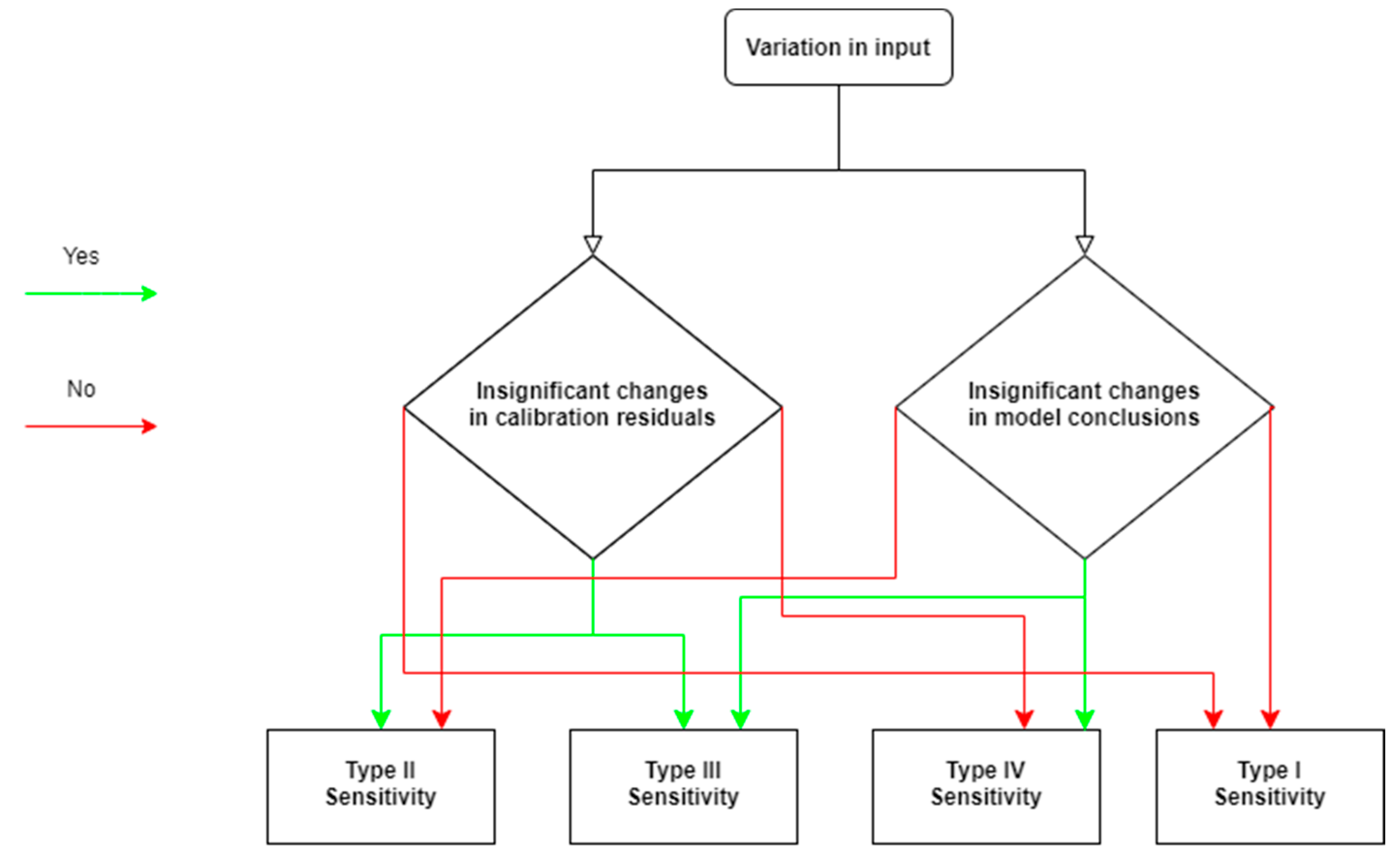
4. Sensitivity Analysis

The sensitivity analysis is the quantification of uncertainty in the output of a model (concentration in this study) based on its inputs. There are many techniques to perform sensitivity analysis. In this study, the sensitivity analysis was performed on the current model using the ASTM Guide technique (1994) [40]. The sensitivity of a model to a variable is classified into four categories, namely Type I, Type II, Type III, and Type IV (see Figure 1 and

Table 3. The categories’ sensitivity analysis and output changes.

	Categories	Changes in Calibration Residuals	Changes in Model Conclusions
Variation in input parameters	Type I	X	X
	Type II	✓	X
	Type III	✓	✓
	Type IV	X	✓

Note: ✓—indicates that there is a change and X—indicates that there is no change.

).

The following steps were followed to complete the sensitivity analysis. Initially, different input parameters were varied to identify the potential sensitive parameters. In the current study q, $u_1$, $u_{*}$, m, a, $b_s{}_{ }$, and $m_t$ were identified parameters to perform the sensitivity analysis. A summary of the ranges for each parameter is given in

Table 4. Ranges of the independent input variable used for the sensitivity analysis.

Run. S. No.	Emission Rate of Pollutants q (g/m/s)	$\mathbf{Wind}\mathbf{Velocity}{\mathit{u}}_1(\mathbf{m}/\mathbf{s})$	Coefficient m	Surface Friction Velocity ${\mathit{u}}_{*}$ (m/s)	Coefficient a	Coefficient ${\mathit{b}}_{\mathit{s} }$	Vertical Spread Due to the Height of the Vehicle ${\mathit{m}}_{\mathit{t}}\left(\mathbf{m}\right)$
1	0.0001	0.9	0.25	0.03	0.32	2.04	0.6
2	0.0024	1.2	0.32	0.04	0.4	2.56	0.7
3	0.003	1.5	0.4	0.06	0.5	3.2	0.8
4	0.0036	1.8	0.48	0.07	0.6	3.84	0.9
5	0.0043	2.1	0.57	0.08	0.72	4.6	1

.

The simulations were executed for each input run varying the variables in the considered range, as given in Table 4. The values were selected based on the possible errors in the specification of each variable. The model calibration values and the predicted output results were generated by running the model. The difference between the predicted output results and the base values were the residuals. The residuals were derived by comparing calculated output results and the output concentration values for the base case input values. The base case input values considered are given in

Table 5. Standard input values considered for sensitivity analysis.

q (g/m/s)	${\mathit{u}}_{1 }$ (m/s)	m	${\mathit{u}}_{* }(\mathbf{m}/\mathbf{s})$	a	${\mathit{b}}_{\mathit{s} }$	${\mathit{m}}_{\mathit{t}}$ (m)
0.0025	1.4	0.57	0.05	0.3	3	0.825

.

The residuals are calculated at three different distances 10 m, 50 m, and 250 m. The graphs were plotted by comparison of variation of input parameters in the considered ranges with the residuals and model conclusions output values. Each variable input parameter was varied to see the change in concentrations for a given downwind distance. The graphs represent the variation in concentration with considered independent variables. The sensitivity analysis for the emission rate of pollutants q, wind velocity $u_1$, the coefficient a, coefficient $b_s{}_{ }$, vertical spread due to the wake caused by the vehicle $m_t$, surface friction velocity $u_{* },$respectively. The type of sensitivity (Type I, Type II, Type III, and Type IV) was determined for each variable parameter depending on changes to the residual values and model conclusion output values. The results are compared and discussed in the results section.

5. Results

The variable parameters considered in the sensitivity analysis were emission rate of pollutant (q), wind velocity at the reference height ($u_1$), coefficient a, coefficient m, coefficient $b_s{}_{ }$, surface friction velocity $(u_{*})$, and additional vertical spread due to the turbulence created by the vehicles ($m_t$). The parameters were vital in describing the sensitivity of the gaseous dispersion model. The plots given in the following figures between the modeled outputs and residuals determined the type of sensitivity for each parameter.

• The sensitivity of model output to the emission rate of pollutants (q):

The graphs are plotted in Figure 2 for the computed concentrations and residuals for three downwind distances. The base case value for emission rate of CO (q) is 0.0025 g/m/s. The plots 2a, 2c, and 2e represent the variation in concentrations, and plots 2b, 2d, and 2f represent residual plots. In the plots between the emission rate of pollutants and output concentrations for each downwind distance, it was observed that the output concentrations increased with an increase in emission rate, as expected. The slope equations and the R² values for a linear fit are mentioned in Figure 2. The calculated concentration and residuals varied with the changes in the input parameter. Significant changes were observed in model conclusions and model residuals at 10 m and 250 m and showed Type III sensitivity (see plots 2a, 2b, 2e, and 2f). At 50 m, a significant change in the model conclusions was observed but the change in calibration results might not be significant (see plots 2c and 2d). These characteristics may lead to Type IV sensitivity instead of Type III sensitivity at 50 m.

• The sensitivity of model output to wind velocity $\left(u_{1 }\right)$:

The graphs for the computed concentrations and residuals for three downwind distances are given in Figure 3. The base case value for wind velocity considered is 1.4 m/s. The plots 3a, 3c, and 3e represent the variation in concentrations, and 3b, 3d, and 3f represent residual plots. These plots showed that output concentrations decreased with an increase in wind velocity. There was a slight increase in the concentration as wind velocity increased at 250 m downwind distance, and it was difficult to explain the increase in concentration with wind velocity. However, the concentrations were decreasing for a given downwind distance for a wind velocity run. The slope equations and the R² values for a linear fit are mentioned in plots in Figure 3. Significant changes were observed in model conclusions and model residuals at 10 m. At 50 m, no significant changes were observed in model conclusions, but there were changes in calibration residuals. Moreover, no significant changes in model conclusions and residuals were observed at 250 m. These characteristics showed that the model was exhibiting Type III sensitivity at 10 m, Type II sensitivity at 50 m, and Type I at 250 m downwind distances. The model equations should be reexamined to check the sensitivity results.

• The sensitivity of model output to the exponent of power-law velocity profile (m):

The graphs are plotted in Figure 4 for the computed concentrations and residuals for three downwind distances. The base case value for the exponent of the power-law velocity profile (m) considered is 0.3. The plots 4a, 4c, and 4e represent the variation in concentrations, and plots 4b, 4d, and 4f represent residual plots. In the plots between the exponent of the power-law velocity profile and output concentrations for different distances, it was observed that the output concentrations decreased with an increase in the exponent of the power-law velocity profile. The slope equations and the R² values for a linear fit are mentioned in plots in Figure 4. Note that the calculated concentration and residuals varied significantly in all cases. Overall, it was observed that there were significant changes in the model conclusions and residuals at 10 m, 50 m, and 250 m. These characteristics showed Type III sensitivity to the exponent of the power-law velocity profile at each downwind distance considered.

• The sensitivity of model output to surface friction velocity ($u_{* }$):

The graphs are plotted in Figure 5 for the computed concentrations and residuals for three downwind distances. The base case value for surface friction velocity ($u_{*})$ considered is 0.05 m/s. The plots 5a, 5c, and 5e represent the variation in concentrations, and plots 5b, 5d, and 5f are for residual plots. In the plots between the surface friction velocity ($u_{*})$ and output concentrations for each downwind distance, it was observed that the output concentrations decreased with an increase in surface friction velocity. The slope equations and the R² values for a linear fit are mentioned in plots in Figure 5. The calculated concentrations and residuals varied significantly. Thus, the model conclusions and residuals changed significantly as the values of friction velocity changed. This model showed Type III sensitivity due to surface friction velocity ($u_{*})$.

• The sensitivity of model output to coefficient a:

The graphs are plotted in Figure 6 for the computed concentrations and residuals for three downwind distances. The base case value for the coefficient a considered is 0.57. The plots 6a, 6c, and 6e represent the variation in concentrations, and plots 6b, 6d, and 6f represent residual plots. In the plots between the coefficient a and output concentrations with incremental distance, it was observed that the output concentrations decreased with an increase in coefficient a, as expected. The slope equations and the R² values for a linear fit are mentioned in plots in Figure 6. The calculated concentration and residuals varied significantly for 10 m, 50 m, and 250 m. These characteristics showed Type III sensitivity to the coefficient a at 10 m, 50 m, and 250 m.

• The sensitivity of model output to coefficient $b_s{}_{ }$:

The graphs are plotted in Figure 7 for the computed concentrations and residuals for three downwind distances. The base case value for coefficient bs considered is 3. The plots 7a, 7c, and 7e represent the variation in concentrations, and plots 7b, 7d, and 7f represent residual plots. In the plots between the coefficient $b_s{}_{ }$ and output concentrations with incremental distance, it was observed that the output concentrations decreased with an increase in the coefficient $b_{s }{.}_{ }$ The slope equations and the R² values for a linear fit are mentioned in plots in Figure 7. The calculated residuals varied significantly with the changes in $b_{s }{.}_{ }$However, it could be observed that there was not much significant change observed in the model conclusions at 10 m, 50 m, and 250 m (see plots 7a, 7c, and 7e), and the model showed Type II sensitivity at all downwind distances to the coefficient $b_s{}_{ }.$

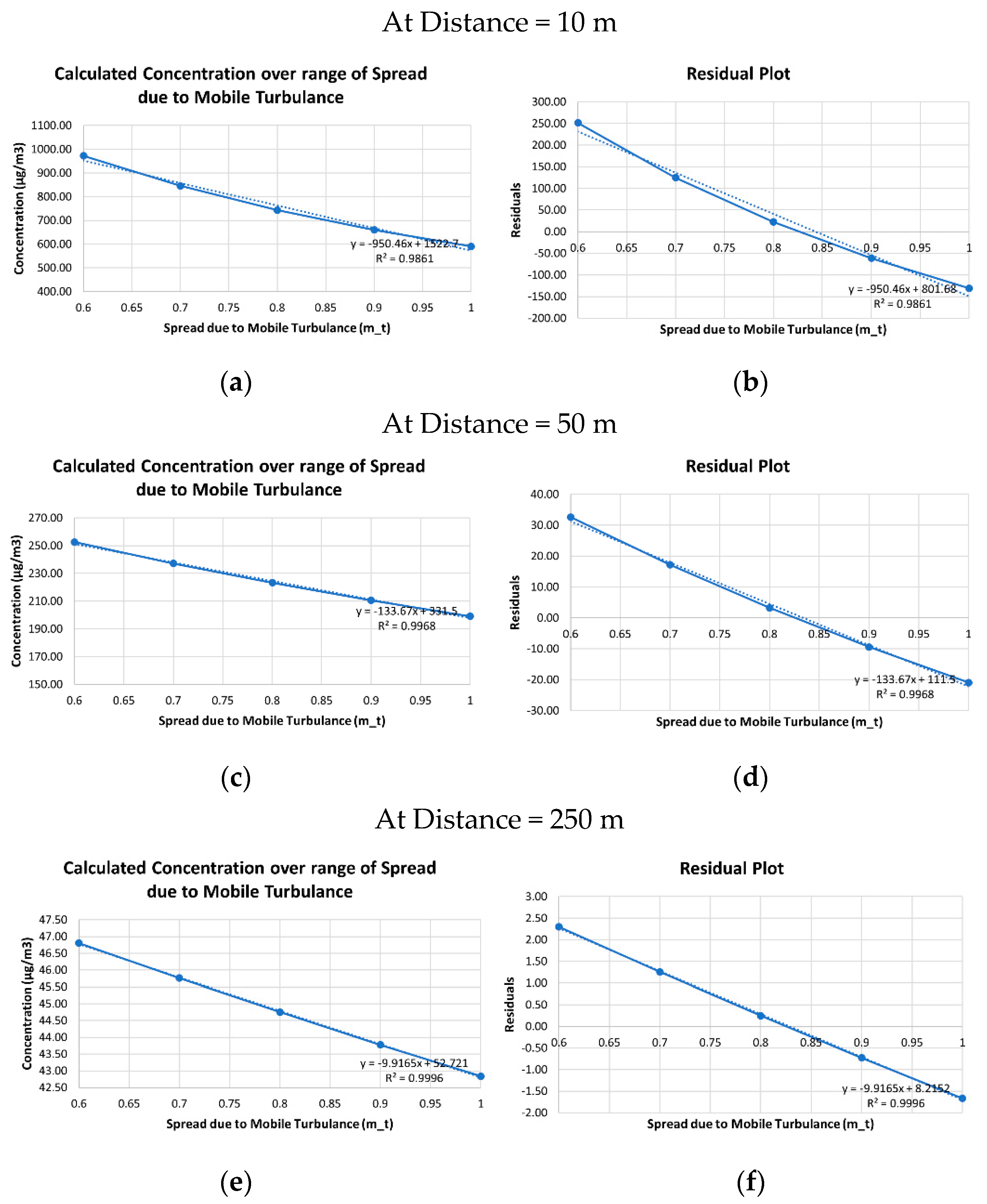
• The sensitivity of model output to the additional spread due to the wake turbulence $m_{t }$:

The graphs are plotted in Figure 8 for the computed concentrations and residuals for three downwind distances. The base case value for $m_{t }$ considered is 0.825. The plots 8a, 8c, and 8e represent the variation in concentrations, and plots 8b, 8d, and 8f represent residual plots. In the plots between $m_{t }$ and output concentrations with incremental distance, it was observed that the output concentrations decreased with an increase in $m_{t }$. It was observed from the plots that there was a significant change in model conclusions and residuals at 10 m and 50 m downwind distances. The calibration residuals at 250 m showed significant change. However, it could be observed that there was not much significant change observed in the model conclusions at 250 m. These characteristics showed Type III sensitivity at 10 m and 50 m. The model showed closer to Type II sensitivity at 250 m.

The above figures show that the model concentrations and residuals changed significantly with the change in the value of the model in most of the cases. A summary of the type of sensitivity of the model is as follows:

• The model shows Type III sensitivity for the emission rate, meteorological variables $m,$ and$u_{*}$, and turbulent variables a and $m_{t }$.
• The sensitivity of the model to the reference wind velocity is Type III, Type II, and Type I depending on the downwind distance.
• The sensitivity of the model is Type II due to coefficient bs.
• Overall, the model equations should be reexamined for$u_1$, $b_{s }$, and $m_{t }$ to make sure that that the model is valid for computing ground level concentrations.

6. Conclusions

A new model SLINE is presented to compute downwind concentrations from line sources on a highway. The sensitivity analysis showed that the model does not exhibit Type III sensitivity for all the input variables. However, the model showed Type III sensitivity for the input parameters q, m, $u_{*}$, a, and $m_t$ in computing concentration at all the downwind distances. One of the vertical spread variables, $b_s$ showed Type II sensitivity. The type of model sensitivity for the reference wind velocity was mixed at different downwind distances. It is important to note that the model formulation should be reexamined for$u_1$, $b_s$, and $m_{t }$ so that the model is not invalidated as outlined in the ASTM Guide (1994). Further study should focus on evaluating the model against the observed data and determining the sensitivity of the model using simultaneous changes in model inputs.

References

1. Wark, K.; Warner, C.F.; Wayne, T.D. Air Pollution: Its Origin and Control; Addison-Wesley: Boston, MA, USA, 1998. [Google Scholar]
2. United Nations Department of Economic and Social Affairs (UN DESA). “68% of the World Population Projected to Live in Urban Areas by 2050”, Says UN, 16 May 2018. Available online: https://www.un.org/development/desa/en/news/population/2018-revision-of-world-urbanization-prospects.html (accessed on 7 November 2020).
3. US EPA. Smog, Soot, and Other Air Pollution from Transportation; US EPA: Washington, DC, USA, 10 September 2015. Available online: https://www.epa.gov/transportation-air-pollution-and-climate-change/smog-soot-and-local-air-pollution (accessed on 7 November 2020).
4. Guidelines for Developing an Air Quality (Ozone and PM2.5) Forecasting Program; EPA-456/R-03-002 June 2003; US EPA: Washington, DC, USA, 2003.
5. Henneman, L.R.; Liu, C.; Mulholland, J.A.; Russell, A.G. Evaluating the effectiveness of air quality regulations: A review of accountability studies and frameworks. J. Air Waste Manag. Assoc. 2017, 67, 144–172. [Google Scholar] [CrossRef]
6. Karroum, K.; Lin, Y.; Chiang, Y.-Y.; Ben Maissa, Y.; El Haziti, M.; Sokolov, A.; Delbarre, H. A Review of Air Quality Modeling. MAPAN J. Metrol. Soc. India 2020, 35, 287–300. [Google Scholar] [CrossRef]
7. Sharma, N.; Chaudhry, K.K.; Rao, C.V.C. Vehicular pollution prediction modelling: A review of highway dispersion models. Transp. Rev. 2004, 24, 409–435. [Google Scholar] [CrossRef]
8. Cook, R.; Isakov, V.; Touma, J.S.; Benjey, W.; Thurman, J.; Kinnee, E.; Ensley, D. Resolving local-scale emissions for modeling air quality near roadways. J. Air Waste Manag. Assoc. 2008, 58, 451–461. [Google Scholar] [CrossRef]
9. Sutton, O.G. Micrometeorology: A Study of Physical Processes in the Lowest Layers of the Earth’s Atmosphere; McGraw-Hill: New York, NY, USA, 1953. [Google Scholar]
10. Stockie, J.M. The Mathematics of Atmospheric Dispersion Modeling. SIAM Rev. 2011, 53, 349–372. [Google Scholar] [CrossRef]
11. Zimmerman, J.R.; Thompson, R.S. User’s Guide for HIWAY: A Highway Air Pollution Model; Office of Research and Development, US Environmental Protection Agency: Washington, DC, USA, 1975.
12. Chock, D.P. A simple line-source model for dispersion near roadways. Atmos. Environ. (1967) 1978, 12, 823–829. [Google Scholar] [CrossRef]
13. Rao, S.T.; Keenan, M.T. Suggestions for Improvement of the EPA-HIWAY Model. J. Air Pollut. Control Assoc. 1980, 30, 247–256. [Google Scholar] [CrossRef]
14. Rao, S.T.; Sistla, G.; Keenan, M.T.; Wilson, J.S. An Evaluation of Some Commonly Used Highway Dispersion Models. J. Air Pollut. Control Assoc. 1980, 30, 239–246. [Google Scholar] [CrossRef]
15. Watson, A.Y.; Bates, R.R.; Kennedy, D. Atmospheric transport and dispersion of air pollutants associated with vehicular emissions. In Air Pollution, the Automobile, and Public Health; National Academies Press: Washington, DC, USA, 1988. [Google Scholar]
16. Heist, D.; Isakov, V.; Perry, S.; Snyder, M.; Venkatram, A.; Hood, C.; Stocker, J.; Carruthers, D.; Arunachalam, S.; Owen, R.C. Estimating near-road pollutant dispersion: A model inter-comparison. Transp. Res. Part D Transp. Environ. 2013, 25, 93–105. [Google Scholar] [CrossRef]
17. Jones, K.; Wilbur, A. A User’s Manual for the CALINE-2 Computer Program; Washington, DC, USA, 1976. [Google Scholar]
18. Benson, P.E. Caline 4—A Dispersion Model for Predicting Air Pollutant Concentrations Near Roadways; The National Academies of Sciences, Engineering, and Medicine: Washington, DC, USA, 1984. [Google Scholar]
19. Eckhoff, P.A.; Braverman, T.N. Addendum to the User’s Guide to CAL3QHC Version 2.0 (CAL3QHCR User’s Guide); Research Triangle Park: Durham, NC, USA, 1995. [Google Scholar]
20. Hall, D.; Spanton, A.; Dunkerley, F.; Bennett, M.; Griffiths, R. A Review of Dispersion Model Inter-comparison Studies Using ISC, R91, AERMOD and ADMS; Environment Agency: Bristol, UK, 2000.
21. Kenty, K.L.; Poor, N.D.; Kronmiller, K.G.; McClenny, W.; King, C.; Atkeson, T.; Campbell, S.W. Application of CALINE4 to roadside NO/NO2 transformations. Atmos. Environ. 2007, 41, 4270–4280. [Google Scholar] [CrossRef]
22. Bluett, J.; Kuschel, G.; Xie, S.; Unwin, M.; Metcalfe, J. The development, use and value of a long-term on-road vehicle emission database in New Zealand. Air Qual. Clim. Chang. 2013, 47, 17. [Google Scholar]
23. Luhar, A.K.; Patil, R. A General Finite Line Source Model for vehicular pollution prediction. Atmos. Environ. (1967) 1989, 23, 555–562. [Google Scholar] [CrossRef]
24. Khare, M.; Sharma, P. Performance evaluation of general finite line source model for Delhi traffic conditions. Transp. Res. Part D Transp. Environ. 1999, 4, 65–70. [Google Scholar] [CrossRef]
25. Boeft, J.D.; Eerens, H.; Tonkelaar, W.D.; Zandveld, P. CAR International: a simple model to determine city street air quality. Sci. Total Environ. 1996, 189, 321–326. [Google Scholar] [CrossRef]
26. Kukkonen, J.; Harkonen, J.; Walden, J.; Karppinen, A.; Lusa, K. Validation of the dispersion model CAR-FMI against measurements near a major road. Int. J. Environ. Pollut. 2001, 16, 137–147. [Google Scholar] [CrossRef]
27. Rao, S.; Sistla, G.; Eskridge, R.; Petersen, W. Turbulent diffusion behind vehicles: Evaluation of ROADWAY models. Atmos. Environ. (1967) 1986, 20, 1095–1103. [Google Scholar] [CrossRef]
28. Bang, H.Q.; Khue, V.H.N.; Tam, N.T.; Lasko, K. Air pollution emission inventory and air quality modeling for Can Tho City, Mekong Delta, Vietnam. Air Qual. Atmos. Health 2018, 11, 35–47. [Google Scholar] [CrossRef]
29. Christoffer, J.; Jurksch, G. The Spatial Distribution of the Average Annual Mean Wind Speed in 10 Meters Height above Ground of the Federal Republic of Germany as a Contribution to the Utilization of Wind Energy. Int. J. Sol. Energy 1984, 2, 469–476. [Google Scholar] [CrossRef]
30. Gokhale, S.; Pandian, S. A semi-empirical box modeling approach for predicting the carbon monoxide concentrations at an urban traffic intersection. Atmos. Environ. 2007, 41, 7940–7950. [Google Scholar] [CrossRef]
31. Milando, C.W.; Batterman, S.A. Operational evaluation of the RLINE dispersion model for studies of traffic-related air pollutants. Atmos. Environ. 2018, 182, 213–224. [Google Scholar] [CrossRef]
32. Bowatte, G.; Lodge, C.J.; Knibbs, L.D.; Erbas, B.; Perret, J.L.; Jalaludin, B.; Morgan, G.G.; Bui, D.S.; Giles, G.G.; Hamilton, G.S.; et al. Traffic related air pollution and development and persistence of asthma and low lung function. Environ. Int. 2018, 113, 170–176. [Google Scholar] [CrossRef] [PubMed]
33. Cai, H.; Xie, S. Traffic-related air pollution modeling during the 2008 Beijing Olympic Games: The effects of an odd-even day traffic restriction scheme. Sci. Total Environ. 2011, 409, 1935–1948. [Google Scholar] [CrossRef] [PubMed]
34. Liang, D.; Golan, R.; Moutinho, J.L.; Chang, H.H.; Greenwald, R.; Sarnat, S.E.; Russell, A.G.; Sarnat, J.A. Errors associated with the use of roadside monitoring in the estimation of acute traffic pollutant-related health effects. Environ. Res. 2018, 165, 210–219. [Google Scholar] [CrossRef] [PubMed]
35. Amoatey, P.; Omidvarborna, H.; Baawain, M.S.; Al-Mamun, A. Evaluation of vehicular pollution levels using line source model for hot spots in Muscat, Oman. Environ. Sci. Pollut. Res. 2020, 27, 31184–31201. [Google Scholar] [CrossRef]
36. US EPA. Air Quality Dispersion Modeling—Preferred and Recommended Models; US EPA: Washington, DC, USA, 2 November 2016.
37. Rao, K.S. Analytical Solutions of a Gradient-Transfer Model for Plume Deposition and Sedimentation; NOAA Technical Memorandum ERL ARL-109; Air Resources Laboratories: Silver Spring, MD, USA, 1981.
38. Nimmatoori, P.; Kumar, A. Development and evaluation of a ground-level area source analytical dispersion model to predict particulate matter concentration for different particle sizes. J. Aerosol Sci. 2013, 66, 139–149. [Google Scholar] [CrossRef]
39. Snyder, M.G.; Venkatram, A.; Heist, D.K.; Perry, S.G.; Petersen, W.B.; Isakov, V. RLINE: A line source dispersion model for near-surface releases. Atmos. Environ. 2013, 77, 748–756. [Google Scholar] [CrossRef]
40. ASTM Guide. Standard Guide for Conducting a Sensitivity Analysis for a Ground-Water Flow Model Application; ASTM Des. 5611-94; ASTM: West Conshohocken, PA, USA, 1994. [Google Scholar]
Figure 1. Flowchart represents the four types of sensitivity analyses.
Environsciproc 04 00017 g001
Figure 2. Variation of concentration with emission rate of pollutants. (a) Model results at 10 m downwind distance; (b) Calibration residuals at 10 m downwind distance; (c) Model results at 50 m downwind distance; (d) Calibration residuals at 50 m downwind distance; (e) Model results at 250 m downwind distance; (f) Calibration residuals at 250 m downwind distance.
Environsciproc 04 00017 g002
Figure 3. Variation of concentration with wind velocity. (a) Model results at 10 m downwind distance; (b) Calibration residuals at 10 m downwind distance; (c) Model results at 50 m downwind distance; (d) Calibration residuals at 50 m downwind distance; (e) Model results at 250 m downwind distance; (f) Calibration residuals at 250 m downwind distance.
Environsciproc 04 00017 g003
Figure 4. Variation of concentration with the exponent of the power-law velocity profile (m): (a) Model results at 10 m downwind distance; (b) Calibration residuals at 10 m downwind distance; (c) Model results at 50 m downwind distance; (d) Calibration residuals at 50 m downwind distance; (e) Model results at 250 m downwind distance; (f) Calibration residuals at 250 m downwind distance.
Environsciproc 04 00017 g004
Figure 5. Variation of concentration with surface friction velocity ( u * ). (a) Model results at 10 m downwind distance; (b) Calibration residuals at 10 m downwind distance; (c) Model results at 50 m downwind distance; (d) Calibration residuals at 50 m downwind distance; (e) Model results at 250 m downwind distance; (f) Calibration residuals at 250 m downwind distance.
Environsciproc 04 00017 g005
Figure 6. Variation of concentration with coefficient a. (a) Model results at 10 m downwind distance; (b) Calibration residuals at 10 m downwind distance; (c) Model results at 50 m downwind distance; (d) Calibration residuals at 50 m downwind distance; (e) Model results at 250 m downwind distance; (f) Calibration residuals at 250 m downwind distance.
Environsciproc 04 00017 g006
Figure 7. Variation of concentration with the coefficient b s   . (a) Model results at 10 m downwind distance; (b) Calibration residuals at 10 m downwind distance; (c) Model results at 50 m downwind distance; (d) Calibration residuals at 50 m downwind distance; (e) Model results at 250 m downwind distance; (f) Calibration residuals at 250 m downwind distance.
Environsciproc 04 00017 g007
Figure 8. Variation of concentration with spread due to mobile turbulence ( m t   ). (a) Model results at 10 m downwind distance; (b) Calibration residuals at 10 m downwind distance; (c) Model results at 50 m downwind distance; (d) Calibration residuals at 50 m downwind distance; (e) Model results at 250 m downwind distance; (f) Calibration residuals at 250 m downwind distance.
Environsciproc 04 00017 g008