Proceeding Paper

Evaluation of Microphysics Schemes in the WRF-ARW Model for Numerical Wind Forecast in José Martí International Airport †

by
Patricia Coll-Hidalgo
1,*,
Albenis Pérez-Alarcón
1,2 and
Pedro Manuel González-Jardines
3
1
Department of Meteorology, Higher Institute of Technologies and Applied Sciences, University of Havana, Havana 10400, Cuba
2
Environmental Physics Laboratory (EPhysLab), CIM-UVigo, Universidade de Vigo, 32004 Ourense, Spain
3
Cuban Corporation of Air Navigation, Havana 10400, Cuba
*
Author to whom correspondence should be addressed.
Presented at the 3rd International Electronic Conference on Atmospheric Sciences, 16–30 November 2020; Available online: https://ecas2020.sciforum.net/.
Environ. Sci. Proc. 2021, 4(1), 31; https://0-doi-org.brum.beds.ac.uk/10.3390/ecas2020-08121
Published: 13 November 2020
(This article belongs to the Proceedings of The 3rd International Electronic Conference on Atmospheric Sciences)

Abstract

:
A sensitivity study was developed with Lin, Morrison 2-moment, weather research and forecasting (WRF) single-moment 5-class (WSM5), and WRF single-moment 6-class (WSM6) microphysics schemes available in the weather research and forecasting-advanced research WRF (WRF-ARW) for the numerical forecast of the wind field at José Martí International Airport, in Cuba. The selection of these schemes was based on their use in numerical weather forecast systems operating in Cuba. As case studies, five storms associated with synoptic patterns that cause dangerous conditions at this aerodrome were selected. The simulations were initialized at 0000 UTC with the forecast outputs of the global forecast system (GFS) model. The schemes were evaluated according to the wind field’s representation in the region where the airport is located, the headlands, and the center of the runway. The errors observed are strongly dependent on the occurrence of convection, especially on the intensity and the factors that cause it. During the dry season (November–April), the lowest errors are observed, while the worst performance is appreciable for the rainy period (May–October). Lin and WSM6 schemes reproduce the best behavior of the wind field on the aerodrome.

1. Introduction

The wind field forecast is one of the most important meteorological supports for air operations. The spatial resolution of meteorological phenomena that modifies the wind field along the runway often exceeds the range of local sensors. Numerical weather prediction (NWP) models are an alternative to be used as alarm systems in aeronautics [1,2,3,4].
The weather research and forecasting (WRF) model [5] is widely used to simulate the near-surface wind for both research and operational applications. It has two dynamic cores, the advanced research WRF (ARW) and the non-hydrostatic mesoscale model (NMM), developed by the National Centre for Atmospheric Research (NCAR) and National Centers for Environmental Prediction (NCEP), respectively. Shaw et al. [2] implemented the WRF-ARW v2.2 model [6] for the Dubai International Airport aviation weather decision support system. The authors installed an operational system assimilating data from satellites, radiometers, wind profiles, radar, and surface observations. In the Hong Kong International Airport, a sub-kilometric NWP capability in capturing low-level wind shear was evaluated [4]. This aviation model (AVM) [7,8] is a sub-kilometer resolution implementation of the WRF.
WRF model offers multiple applications and, like most of NWPs, several physics options. For wind forecast, commonly, sensitivity boundary-layer parametrizations (PBL) studies were developed [9,10,11,12,13,14,15,16,17]. In Cuba, the meteorological model WRF-ARW sensitivity to physics options was tested [18,19]. The prediction systems SiSPI [20] and SPNOA [21] were developed and implemented in the Center of Atmospheric Physics of the Institute of Meteorology of Cuba, but not specific to the aviation application. For this purpose, Díaz-Zurita et al. [22] improved a numerical wind surface derived from WRF-NMM for José Martí International Airport. This airport is located near the elevations of Cacahual. The catabatic flow modifies the characteristics of the meteorological variables at the aerodrome and its vicinity [23]. Furthermore, at this aerodrome, Sosa [24] points out that storms in the vicinity of the aerodrome usually originate dangerous phenomena associated with wind field variations.
Microphysics parametrizations are significant in predicting storms, as is described in many types of research [25,26,27,28,29]. To provide a preliminary evaluation of numerical wind field forecast over José Martí International Airport, a sensitivity study was developed. From WRF practice recommendations [30], ARW core was used in this research. Based on results that show the influence of storms in aerodrome vicinity wind field variations, different microphysics schemes’ capability to represent these changes was verified.
Study Area and Case Studies
Barcía et al. [31] divided Cuba into forecast regions according to the behavior of the meteorological variables recorded in the observational meteorological network. The regions are classified according to the extreme temperatures, the influence of the sea breeze, and the physical–geographical characteristics. José Martí International Airport is located in the inland forecast region of the Artemisa, Havana, and Mayabeque provinces (Figure 1a).
This airport has a 4 km runway (Figure 1b), with a southeast–northeast orientation. The airport is surrounded by terrain with complex orography. At the aerodrome, there is a catabatic flow of moist air that favors a drop in temperatures around the runway [23].
Sosa [24] used meteorological data from observations in the José Martí International Airport during the period between 2012 and 2017 to describe the behavior of the low-level wind shear. This hazardous phenomenon for aircraft is associated with meteorological systems: cold front (18.36%), anticyclone (53.06%), and tropical wave (10.20%) [24]. The author identified the following synoptic patterns as the most frequent in which low-level wind shear occurs:
  • Influence of the North Atlantic Subtropical Anticyclone with trough medium and high levels;
  • Influence of the North Atlantic Subtropical Anticyclone in the entire tropospheric column;
  • Migratory anticyclones;
  • Tropical waves into the south of western Cuba.
  • Cold fronts on western Cuba.
Sosa [24] refers to that significant wind field variations over the airport are often reported under storms. As case studies, five storms associated with synoptic patterns that cause dangerous conditions at this aerodrome were selected (Table 1).

2. Materials and Methods

2.1. Numerical Experiments

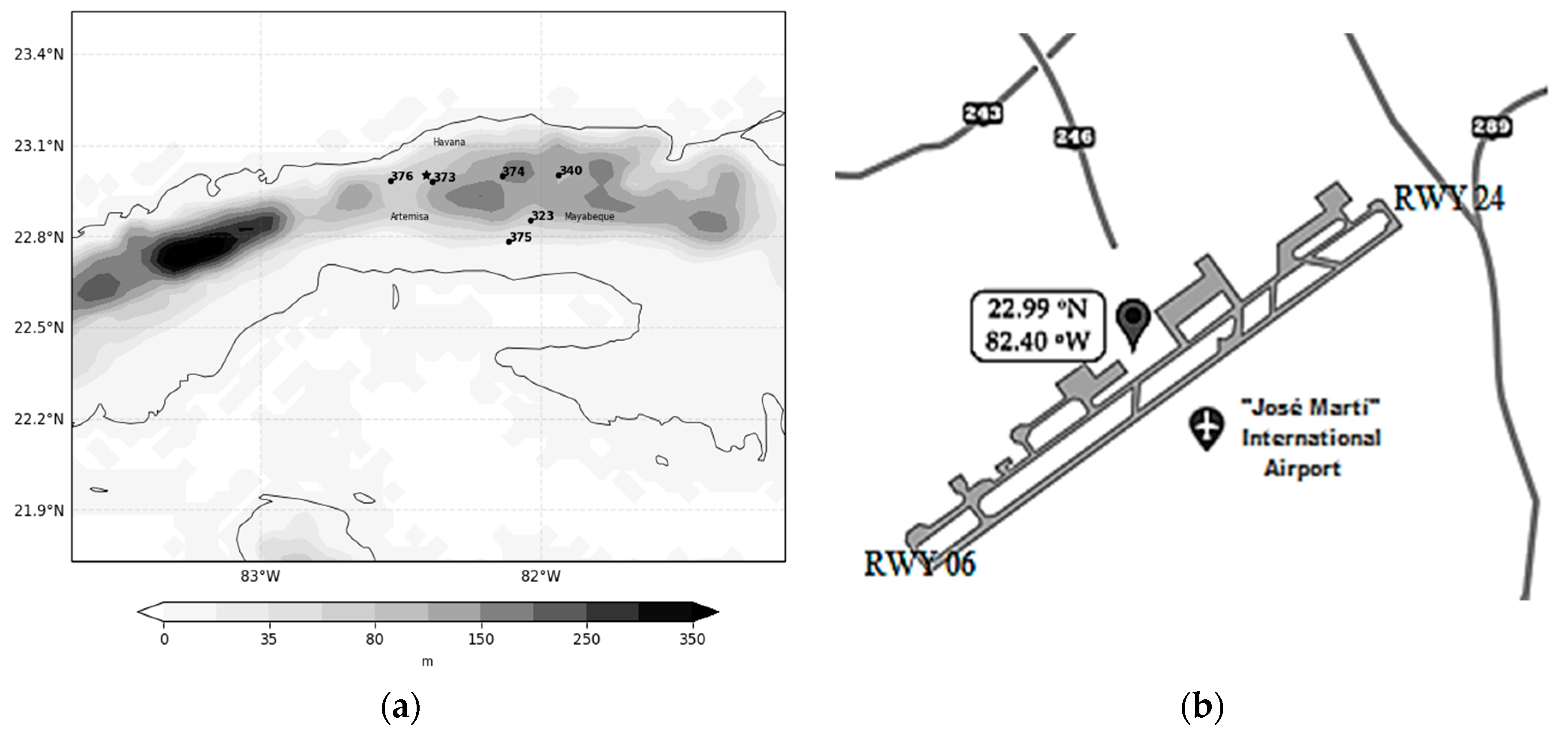
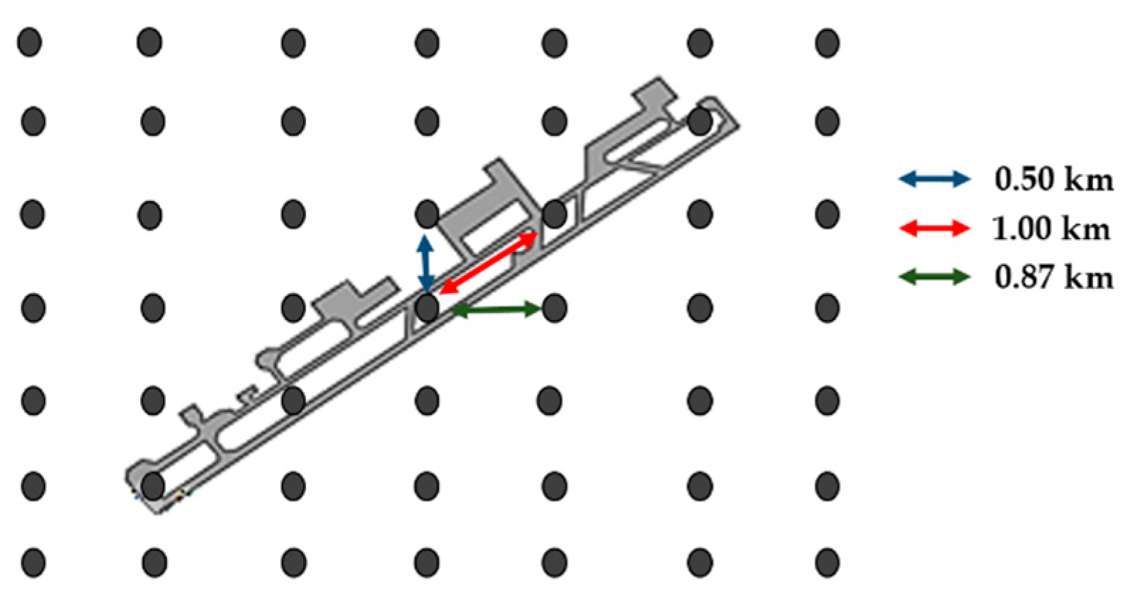
2.1.1. Model and Domain Configuration

The WRF v.3.9 model was used with ARW dynamic core. The simulations comprised 12-4km two-way nested domains (Figure 2) and 34 verticals levels. Briefly, the setup includes for both domains: Rapid Radiative Transfer Model longwave radiation parametrization [32], Dudhia shortwave radiation scheme [33], Unified Noah land-surface model [34], Grell–Freitas ensemble cumulus parametrization [35], Mellor–Yamada–Janjić planetary boundary layer [36]. The model was initialized and forced at the boundaries by a 0.500 GFS forecast, with every 3 hourly updated boundary conditions.

2.1.2. Experimental Design

Storms simulations were performed with four selected microphysics schemes: Lin [36], Morrison 2-moment [37], WSM5 [38], and WSM6 [39]. Table 2 shows the main species of prognostic variables in these schemes. The selection was based on their use and performance in numerical weather forecast systems operating in Cuba [18,19]. The forecasts were for 54 h, started from the storm observation date at 0000 UTC.

2.2. Data and Methodology

2.2.1. Data

Wind data observations were obtained from weather stations placed in the study area (Figure 1a). The model was initialized with the GFS forecast, which is freely available at https://nomads.ncep.noaa.gov/cgi-bin/filter_gfs_0p50.pl (accessed on 15 January 2020). On the other hand, radars products were obtained from the Key West, Florida, USA (KBYX) doppler radar (available online at https://www.ncdc.noaa.gov/nexradinv/chooseday.jsp?id=kbyx (accessed on 15 Janaury 2020)). In addition, the software NOAA Weather and Climate Toolkit v.4.5.0 (free available at https://www.ncdc.noaa.gov/wct/install.php (accessed on 12 Febraury 2020)) was utilized to analyze the radar data.

2.2.2. Postprocessing WRF-ARW Output Files

In this paper, it was used the WRF-ARW output variables REFL_10CM (dBZ), T2 (K), PSFC (Pa), Q2 (kg kg−1), U10 (x-component) and V10 (y-component) (m s−1). Surface wind speed was computed from the output of wind components.
In the domain of 4 km (d02) of the resolution, the density of the nodes in the neighborhood of the airport is low. For this reason, the rectangular grid developed by Díaz-Zurita et al. [22] was used. This grid takes into account the orientation (60 from the horizon) and the length of the runway (4 km). Five points are matched: one in the center of the runway (MID), one at each headland, and the other two points at 1 km from the center. The grid with a longitudinal resolution of 0.87 km and a latitudinal resolution of 0.5 km is shown in Figure 3.
Based on the results of Díaz-Zurita et al. [22], for wind interpolation, the natural neighbor method was used. In addition, following Díaz-Zurita et al.’s [22] recommendations, a correction to the interpolated wind field is applied with a consistent mass model.
This model is based on the equation of continuity for an incompressible air mass moving in a two-dimensional domain, Ω, with a velocity field u ( u , v , w ) :
p t + · ( ρ u ) = 0 ,
If the constant air density is considered for the entire domain, the equation becomes:
· u = 0 Ω ,
which joins the impenetrability condition on the ground Γ b , thus constituting the boundary condition:
η · u = 0 Γ b ,
From conditions (2) and (3), the consistent mass models pose a least-squares problem with the velocities to adjust u ( u , v , w ) from the observed u 0 ( u 0 , v 0 , w 0 ) in the Ω domain, according to the functional:
E ( u , v , w ) = [ α 1 2 ( u u 0 ) 2 + α 2 2 ( v v 0 ) 2 + α 3 2 ( w w 0 ) 2 ] d x d y d z ,
where { u ( x , y , z ) , v ( x , y , z ) , and w ( x , y , z ) , } are the wind components calculated by the model through fit; { u 0 ( x , y , z ) , v 0 ( x , y , z ) , and w 0 ( x , y , z ) , } are the components of the initial field, interpolated from the observations, and α 1 , α 2 , α 3 are the Gaussian precision modules [40]. Considering α 1 and α 2 identical, for horizontal directions, the functional to minimize (4) is:
E ( u , v , w ) = [ α 1 2 ( u u 0 ) 2 + ( v v 0 ) 2 + α 2 2 ( w w 0 ) 2 ] d x d y d z ,
The search field v ( u , v , w ) will be the solution to the problem:
Find v ∈ K such that,
E ( v ) = E u K m i n ( u ) , K = { u ; · u = 0 , n · u Γ b } ,
This problem is equivalent to finding the saddle point at ( u , Φ ) of the Lagrangian:
L ( u , λ ) = E ( u ) + λ · u d Ω ,
The technique of Lagrange multipliers allows obtaining the saddle point of the expression (8), L ( u , λ ) L ( u , Φ ) L ) such that the solution field is obtained from the Euler-Lagrange equations:
v = v 0 + T Φ ,
where Φ is the Lagrange multiplier and T = [ T h , T h , T v ] is the diagonal transmission tensor:
T h = 1 2 α 1 2 T v = 1 2 α 2 2 ,
u = u 0 + T h Φ x , v = v 0 + T h Φ y , w = w 0 + T v Φ z ,
If α 1 , α 2 are considered constant throughout the domain, the variational formulation leads to an elliptic equation defined in Φ. Indeed, substituting Equation (8) in (2) results:
· ( T ) = · u 0 ,
which is completed by the null Dirichlet condition at permeable boundaries (vertical domain boundaries)
Φ = 0 Γ a ,
and Neumann’s condition in the raincoats (terrain and upper border)
n · Φ = n · v 0 Γ b ,
Considering T h and T v constant, Equation (11) becomes:
Φ 2 x 2 + Φ 2 y 2 + T v T h Φ 2 z 2 = 1 T h ( u 0 x + v 0 y + w 0 z ) ,
eliminating the vertical component (two dimensions) was obtained:
Φ 2 x 2 + Φ 2 y 2 = 1 T h ( u 0 x + v 0 y ) ,
This methodology guarantees the conservation of wind direction due to the impenetrability conditions.
To evaluate the radar’s basic features and structure simulation of storms, verticals profiles of reflectivity and relative humidity were generated. Relative humidity was determined using Clausius–Clapeyron [41] (Equation 1):
R H = 0.263 p q [ e x p 17.67 ( T T 0 ) T 29.65 ] 1 ,
where:
  • T = temperature (K);
  • p = pressure (Pa);
  • q = specific humidity or the mass mixing ratio of water vapor to total air (dimensionless);
  • T0 = reference temperature (typically 273.16 K) (K).
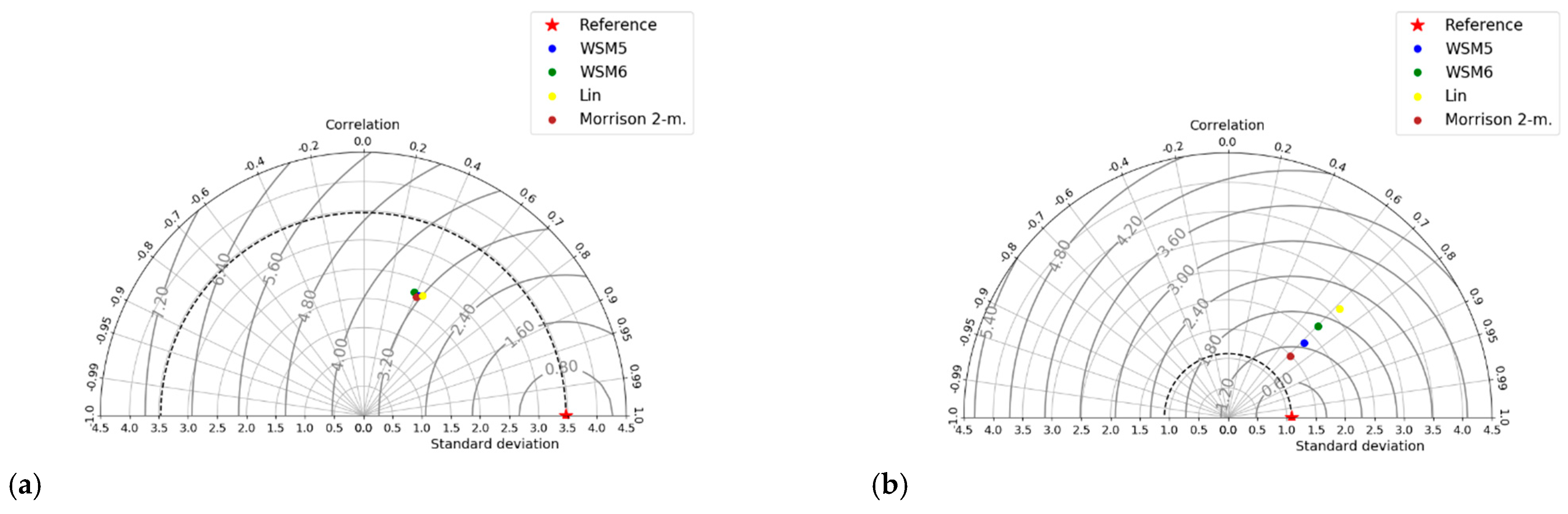
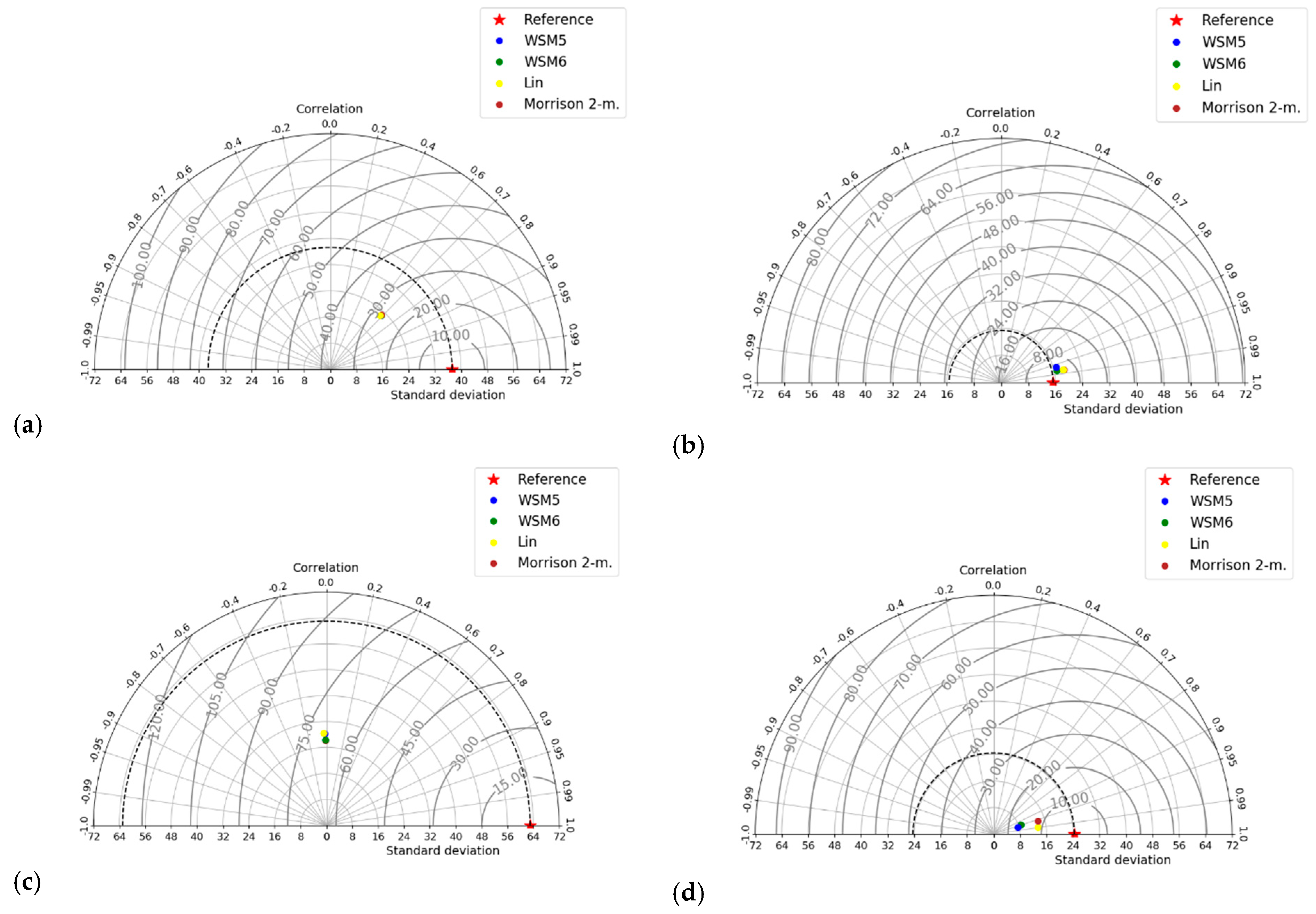
2.2.3. Evaluation

The model output was compared with meteorological observations. In this work, the forecast verification was calculated some statistical metrics: mean systematic error or BIAS, mean absolute error (MAE), root-mean-squared error (RMSE), and Pearson’s correlation coefficient (rp). To obtain the best microphysics scheme to reproduce the surface wind properties derived from storms, the analysis was developed pre-, in- and after- the occurrence of the event [29].

3. Results and Discussion

3.1. Convective Storm Analysis

The late afternoon ground heat flux, the inland breeze convergence, and high-pressure levels diffluence origins the storm of 29 June 2012. Particularly, this storm caused the highest wind speeds records on the runway. At 2:00 pm local time (18:00 UTC), the storm had a maximum height of 13.91 km and a core of maximum reflectivity of 60.5 dBZ at 4.37 km. The spatial pattern of maximum reflectivity, vertical profile mixing ratio of hydrometeor particles, and postprocessed wind field are presented for the tested microphysics schemes when the storm occurred (Figure 4). WSM5 (Figure 4g) and WSM6 (Figure 4j) simulated high maximum reflectivity (50–55 dBZ) in the nearest location as radar did (22.978, −82.345). Both Lin and WSM6 schemes produced more than one core cloud echo. That behavior of WSM6 was founded previously by Sari, Pulung, and Sukma [29] for a hail event study case in Surabaya, Indonesia.
The postprocessed wind field for each scheme is presented; similar predicted wind speeds and directions were shown by WSM5 (Figure 4i) and WSM6 (Figure 4l). The authors reported that the microphysics schemes were not sensitive to surface properties (main wind flow in particular) and suggested a non-sensitivity of wind direction to microphysics parameterization [28,29]. However, convective storms develop were sensitive to the microphysics schemes [42,43,44,45,46]. Figure 4 shows the differences in the postprocessed wind fields. The WSM5 and WSM6 wind fields are quite similar, which can be linked with the position and size of the simulated storm.
Figure 4 also shows vertical simulated hydrometeor profiles; perceptible variations were observed. All schemes predicted mixing ratios of hydrometeors only for warm cloud processes, which is likely to occur in Cuba. WSM6 (Figure 4k) scheme shows the best radars basics features among the schemes. In the first place, WSM6 produces more graupels than the other schemes; second, WSM6 presented the greatest decrease in the vapor mixing ratio near 7 km, when the rest of the diagrams show it over 5 km; and finally, WSM6 also had the highest rain mixing ratio, which decreased with increasing height, from the surface to 6 km.

3.2. Wind Field Simulation

Figure 5 and Figure 6 show skills metrics for forecasting wind speed and direction pre-, in- and after- the occurrence of storms selected as case studies. In the rainy season storms, for the wind speed and wind direction forecasts, the highest biases are shown in the presence of storms (Table 3). In the case studies, the occurrence of several mesoscale convective cells caused the heterogeneous distribution of the wind speed and direction.
In addition, during storms, the biggest differences in skills metrics for wind direction were obtained. This variable was underestimated. On the runway, the error measurements were more dispersed, both for speed (Figure 5d) and direction (Figure 6d). This may have been a consequence of the different simulated storm positions and characteristics from each tested microphysics. To consider the best microphysical scheme, this analysis remains difficult. However, WSM6 and Lin occasionally exhibit better scores. Previously research for this study area [25] report that WSM6 has a skill for wind forecast.
For the dry season, the lowest biases in the wind speed forecast were observed during the occurrence of storms, as summarized in Table 4. In the case of wind direction, the highest biases are seen at this time. This behavior was similar to that observed during the rainy season. Skills metrics indicate a more accurate forecast than in the rainy season. The fundamental difference between the cases was in the origin of the storms.
In the dry season, Pearson’s correlation in the region reached values of up to 0.6, as it is shown in Figure 7. On the runway, the Pearson’s correlations ranged between 0.7 and 0.99 (Figure 8d), which suggests the model’s ability to represent changes in wind direction, probably due to mass consistent correction applications. Once more, the schemes show fewer differences among themselves. The forecast errors may also be attributed to a lateral boundary condition, which was obtained from 0.50 × 0.50 horizontal resolution of the GFS forecast data.

4. Conclusions

A sensitivity study was developed with Lin, Morrison 2-moment, WSM5, and WSM6 microphysics schemes for the wind field’s numerical forecast at José Martí International Airport. As case studies, five storms associated with synoptic patterns that cause dangerous conditions at this aerodrome were selected. The sensitivity of the microphysics scheme using the WRF model on 29 June 2012, was discussed. It is important to note that WSM6 showed the most realistic storm radar features and vertical profile hydrometeors, also, it represented distributions according to warm cloud processes, which are likely to occur in Cuba. In general , we obtain that the wind field was modified by the position and size of the simulated storms.
Furthermore, skills metrics pre-, in- and after- storms were obtained. Between seasons was observed pronounced differences in errors, possibly linked to dissimilarities in storms genesis conditions. Skills metrics indicated a more accurate forecast in dry season storms than in the rainy season ones. Additionally, the consistent mass correction application may cause higher correlations between wind directions forecast at the runway.
To consider the best microphysical scheme, this analysis remains difficult. However, WSM6 showed better scores in the major criterion of the study developed. Nevertheless, these results are the first attempt to obtain the best configuration of the WRF model for numerical storm forecasts in the airport. Ongoing work will, therefore, include other sensitivity meteorological field analyses.

Author Contributions

Conceptualization, P.C.-H. and P.M.G.-J.; methodology, P.C.-H.; software, P.C.-H.; A.P.-A. and P.M.G.-J.; validation, P.C.-H.; formal analysis, P.C.-H.; investigation, P.C.-H. and A.P.-A.; data curation, P.C.-H. and P.M.G.-J.; writing—original draft preparation, P.C.-H.; writing—review and editing, P.C.-H. and A.P.-A.; visualization, P.C.-H. and A.P.-A.; supervision, A.P.-A. and P.M.G.-J. All authors have read and agreed to the published version of the manuscript.

Funding

This research received no external funding.

Acknowledgments

Authors would like to thank NOAA for freely available GFS forecast data and Key West radar data.

Conflicts of Interest

The authors declare no conflict of interest.

References

  1. Boilley, A.; Mahouf, J.-F; Lac, C. High resolution numerical modeling of low level wind-shear over the Nice-Ĉote d’ Azur Airport. In Proceedings of the 13th AMS Conference on Mountain Meteorology, Whistler, BC, Canada, 11–15 August 2018; pp. 11–15. [Google Scholar]
  2. Shaw, B.; Spencer, P.; Carpenter, J.; Barrere, J. Implementation of the WRF model for the Dubai International Airport aviation weather decision support system. In Proceedings of the 13th Conference on Aviation, Range and Aerospace Meteorology, New Orleans, LA, USA, 2008. 5.2. [Google Scholar]
  3. Urlea, A.-D.; Pietrisi, M. Study of the Low Level Wind Shear using AMDAR reports. J. Geophys. Res. 2015, 17, 2015–2185. [Google Scholar]
  4. Hon, K.-K. Predicting Low-Level Wind Shear Using 200-m-Resolution NWP at the Hong Kong International Airport. J. Appl. Meteorol. Clim. 2020, 59, 193–206. [Google Scholar] [CrossRef]
  5. Skamarock, W.C.; Klemp, J.B.; Dudhia, J.; Grill, D.O.; Barker, D.M.; Duda, M.G.; Huang, X.-Y.; Wang, W.; Powers, J.G. A Description of the Advanced Research WRF Version 3; NCAR Tech Note NCAR/TN 475 STR; UCAR Communications: Boulder, CO, USA, 2008. [Google Scholar] [CrossRef]
  6. Shamarock, W.C.; Klemp, J.B.; Dudhia, J.; Gill, D.O.; Barker, M.; Wang, W.; Powers, J.G. A Description of the Advanced Research WRF Version 2; NCAR Tech Note NCAR/TN 468 STR; National Center for Atmosferic Research: Boulder, CO, USA, 2005. [Google Scholar]
  7. Chan, P.W.; Hon, K.K. Performance of super high resolution numerical weather prediction model in forecasting terrain-disrupted airflow at the Hong Kong International Airport: Case studies. Meteorol. Appl. 2015, 23, 101–114. [Google Scholar] [CrossRef]
  8. Hon, K.K. Simulated satellite imagery at sub-kilometre resolution by the Hong Kong Observatory. Weather 2018, 73, 139–144. [Google Scholar] [CrossRef]
  9. Srinivas, C.V.; Venkatesan, R.; Bagavath Singh, A. Sensitivity of mesoscale simulations of land-sea breeze to boundary layer turbulence parameterization. Atmos. Environ. 2007, 41, 2534–2548. [Google Scholar] [CrossRef]
  10. Miao, J.-F.; Wyser, K.; Chen, D.; Ritchie, H. Impacts of boundary layer turbulence and land surface process parameterizations on simulated sea breeze characteristics. Ann. Geophys. 2009, 27, 2303–2320. [Google Scholar] [CrossRef]
  11. Storm, B.; Basu, S. The WRF Model Forecast-Derived Low-Level Wind Shear Climatology over the United States Great Plains. Energies 2010, 3, 258–276. [Google Scholar] [CrossRef]
  12. Hu, X.-M.; Nielsen-Gammon, J.W.; Zhang, F. Evaluation of Three Planetary Boundary Layer Schemes in the WRF Model. J. Appl. Meteorol. Clim. 2010, 49, 1831–1844. [Google Scholar] [CrossRef]
  13. Carvalho, D.; Rocha, A.; Gómez-Gesteira, M.; Santos, C.S. A sensitivity study of the WRF model in wind simulation for an area of high wind energy. Environ. Model. Softw. 2012, 33, 23–34. [Google Scholar] [CrossRef]
  14. Hu, X.-M.; Klein, P.M.; Xue, M. Evaluation of the updated YSU planetary boundary layer scheme within WRF for wind resource and air quality assessments. J. Geophys. Res. Atmos. 2013, 118. [Google Scholar] [CrossRef]
  15. García-Diez, M.; Fernández, J.; Fitaand, L.; Yague, C. Seasonal dependence of WRF model biases and sensitivity to PBL schemes over Europe. Q. J. R. Meteorol. Soc. 2013, 139, 501–514. [Google Scholar] [CrossRef]
  16. Madala, S.; Satyanarayana, A.; Rao, T.N. Performance evaluation of PBL and cumulus parameterization schemes of WRF ARW model in simulating severe thunderstorm events over Gadanki MST radar facility—Case study. Atmospheric Res. 2014, 139, 1–17. [Google Scholar] [CrossRef]
  17. Boadh, R.; Satyanarayana, A.; Krishna, T.V.B.P.S.R.; Madala, S. Sensitivity of PBL schemes of the WRF-ARW model in simulating the boundary layer flow parameters for their application to air pollution dispersion modeling over a tropical station. Atmósfera 2016, 29, 61–81. [Google Scholar] [CrossRef]
  18. Sierra, M.; Borrajero, L.; Ferrer, A. L.; Morfa, Y.; Yordanis, A.; Loyola, M.; Hinojosa, M. Sensitivity studies of the SisPI to changes in the PBL, the number of vertical levels and the microphysics and clusters parameterizations, at very high resolution. Tech. Sci. Rep. 2017. [CrossRef]
  19. Sánchez, E.O. Evaluation of the medium-term forecast of the atmospheric component of the SPNOA with data from INSMET meteorological stations. Bachelor’s Thesis, Higher Institute of Technologies and Applied Sciences, Havana, Cuba, 2018. [Google Scholar]
  20. Sierra, L.M.; Ferrer HA, L.; Valdés, R.; Mayor, G.Y.; Cruz RR, C.; Borrajero, M.I.; Rodríguez GC, F.; Rodríguez, N.; Roque, A. Automatic mesoscale prediction system of four daily cycles. Tech. Sci. Rep. 2015. [CrossRef]
  21. Pérez-Bello, A.; Mitrani, A.I.; Díaz, R.O.; Wettre, C.; Robert, L.H. A numerical prediction system combining ocean, waves and atmosphere models in the Inter-American Seas and Cuba. Rev. Cub. Meteor. 2019, 25, 109–120. [Google Scholar]
  22. Díaz-Zurita, A.; Góngora-González, C.M; Lobaina-La, O.A.; Pérez-Alarcón, A.; Coll-Hidalgo, P. Numerical mesoscale and short-term wind forecast for the “José Martí” International Airport of Havana. J. Braz. Meteor. in press.
  23. Grillo, N. The fog at the “José Martí” International Airport, its relationship with events and meteorological variables. Bachelor’s Thesis, Higher Institute of Technologies and Applied Sciences, Havana, Cuba, 2013. [Google Scholar]
  24. Sosa, A. International Airport “José Martí” low-level wind shear characteristics during 2012–2017 period. Bachelor’s Thesis, Higher Institute of Technologies and Applied Sciences, Havana, Cuba, 2018. [Google Scholar]
  25. Rajeevan, M.; Kesarkar, A.; Thampi, S.B.; Rao, T.N.; Radhakrishna, B.; Rajasekhar, M. Sensitivity of WRF cloud microphysics to simulations of a severe thunderstorm event over Southeast India. Ann. Geophys. 2010, 28, 603–619. [Google Scholar] [CrossRef]
  26. Han, J.-Y.; Baik, J.-J.; Khain, A.P. A Numerical Study of Urban Aerosol Impacts on Clouds and Precipitation. J. Atmospheric Sci. 2012, 69, 504–520. [Google Scholar] [CrossRef]
  27. Halder, M.; Hazra, A.; Mukhopadhyay, P.; Siingh, D. Effect of the better representation of the cloud ice-nucleation in WRF microphysics schemes: A case study of a severe storm in India. Atmospheric Res. 2015, 154, 155–174. [Google Scholar] [CrossRef]
  28. Shrestha, R.K.; Connolly, P.J.; Gallagher, M.W. Sensitivity of WRF Cloud Microphysics to Simulations of a Convective Storm over the Nepal Himalayas. Open Atmos. Sci. J. 2017, 11, 29–43. [Google Scholar] [CrossRef]
  29. Sari, F.P.; Baskoro, A.P.; Hakim, O.S. Effect of different microphysics scheme on WRF model: A simulation of hail event study case in Surabaya, Indonesia. AIP Conf. Proc. 2018, 1987, 020002. [Google Scholar] [CrossRef]
  30. Dudhia, J.; Wang, J. WRF Advanced Usage and Best Practices. In Proceedings of the 16th WRF Annual Workshop, Boulder, CO, USA, 10–11 June 2014; Available online: https://www2.mmm.ucar.edu/wrf/users/workshops/WS2014/ppts/best_prac_wrf.pdf (accessed on 8 July 2020).
  31. Barcía, S.; Ballester, M.; Cedeño, Y.; García, E.; González, J.; Regueira, V. Time-space variability of the variables that intervene in short-term forecasts in Cuba. Technical Scientific Report of the Institutional Project: Evaluation of weather forecasts, 2012, 36–45, Instituto de Meteorología de la República de Cuba, Havana, Cuba.
  32. Mlawer, E.J.; Taubman, S.J.; Brown, P.D.; Iacono, M.J.; Clough, S.A. Radiative transfer for inhomogeneous atmospheres: RRTM, a validated correlated-k model for the longwave. J. Geophys. Res. Space Phys. 1997, 102, 16663–16682. [Google Scholar] [CrossRef]
  33. Dudhia, J. Numerical study of convection observed during the winter monsoon experiment using a mesoscale two-dimensional model. J. Atmos. Sci. 1989, 46, 3077–3107. [Google Scholar] [CrossRef]
  34. Tewari, M.; Chen, F.; Wang, W.; Dudhia, J.; LeMone, M.A.; Mitchell, K.; Ek, M.; Gayno, G.; Wegiel, J.; Cuenca, R.H. Implementation and verification of the unified NOAH land surface model in the WRF model. In Proceedings of the 20th Conference on Weather Analysis and Forecasting/16th Conference on Numerical Weather Prediction, Seattle, WA, USA, 12 January 2004; pp. 11–15. [Google Scholar]
  35. Grell, G.A.; Freitas, S.R. A scale and aerosol aware stochastic convective parameterization for weather and air quality modeling. Atmospheric Chem. Phys. Discuss. 2014, 14, 5233–5250. [Google Scholar] [CrossRef]
  36. Janjić, Z.I. Nonsingular Implementation of the Mellor-Yamada Level 2.5 Scheme in the NCEP Meso Model. NCEP Office Note o. 437, 2002. Available online: https://repository.library.noaa.gov/view/noaa/11409 (accessed on 8 July 2020).
  37. Lin, Y.-L.; Farley, R.D.; Orville, H.D. Bulk parameterization of the snow field in a cloud model. J. Climate Appl. Meteor. 1983, 22, 1065–1092. [Google Scholar] [CrossRef]
  38. Morrison, H.; Thompson, G.; Tatarskii, V. Impact of Cloud Microphysics on the Development of Trailing Stratiform Precipitation in a Simulated Squall Line: Comparison of One- and Two-Moment Schemes. Mon. Weather. Rev. 2009, 137, 991–1007. [Google Scholar] [CrossRef]
  39. Hong, S.Y.; Dudhia, J.; Chen, S.H. A revised approach to ice microphysical processes for the bulk parameterization of clouds and precipitation. J. Amer. Met. Soc. 2004, 132, 103–120. [Google Scholar] [CrossRef]
  40. Hong, S.-Y.; Lim, K.-S.S.; Lee, Y.-H.; Ha, J.-C.; Kim, H.-W.; Ham, S.-J.; Dudhia, J. Evaluation of the WRF Double-Moment 6-Class Microphysics Scheme for Precipitating Convection. Adv. Meteorol. 2010, 2010, 1–10. [Google Scholar] [CrossRef]
  41. Montero, G.; Montenegro, R.; Escobar, J.; Rodríguez, E.; González, J. Modeling and Numerical Simulation of Wind Fields Oriented to Air Pollution Processes; University of Las Palmas: Las Palmas, Spain, 2006. [Google Scholar]
  42. Iribarne, J.V.; Godson, W.L. Atmospheric Thermodynamics. In Geophysics and Astrophysics Monographs, 2nd ed.; McCormac, B.M., Ed.; Kluwer Academic Publishers: Boston, MA, USA, 1981; p. 259. [Google Scholar]
  43. Reisner, J.; Rasmussen, R.M.; Bruintjes, R.T. Explicit forecasting of supercooled liquid water in winter storms using the MM5 mesoscale model. Q. J. R. Meteorol. Soc. 1998, 124, 1071–1107. [Google Scholar] [CrossRef]
  44. Liu, C.; Moncrieff, M.W. Sensitivity of Cloud-Resolving Simulations of Warm-Season Convection to Cloud Microphysics Parameterizations. Mon. Weather. Rev. 2007, 135, 2854–2868. [Google Scholar] [CrossRef]
  45. Otkin, J.A.; Greenwald, T.J. Comparison of WRF Model-Simulated and MODIS-Derived Cloud Data. Mon. Weather. Rev. 2008, 136, 1957–1970. [Google Scholar] [CrossRef]
  46. Liu, C.; Ikeda, K.; Thompson, G.; Rasmussen, R.; Dudhia, J. High-Resolution Simulations of Wintertime Precipitation in the Colorado Headwaters Region: Sensitivity to Physics Parameterizations. Mon. Weather. Rev. 2011, 139, 3533–3553. [Google Scholar] [CrossRef]
Figure 1. Study area (Artemisa–Havana–Mayabeque) (a) Topography (shaded) and meteorological observational stations (markers) (b) José Martí International Airport runway.
Environsciproc 04 00031 g001
Figure 2. Simulations domains.
Environsciproc 04 00031 g002
Figure 3. Rectangular grid resolution.
Environsciproc 04 00031 g003
Figure 4. 29 June 2012 storm: panels from left to right are the spatial patterns of maximum reflectivity, vertical profile mixing ratio of hydrometeor particles and postprocessed wind field: (a-c) Lin; (d-f) Morrison 2-moment; (g-i) WSM5; (j-l) WSM6.
Environsciproc 04 00031 g004
Figure 5. Taylor diagrams for rainy season wind speed forecast. Panels from left to right inland region errors measurements and runway error measurements: (a,b) pre-; (c,d) in-; (e,f) after- storm.
Environsciproc 04 00031 g005
Figure 6. Taylor diagrams for rainy season wind direction forecast, panel from left to right inland region errors measurements and runway error measurements: (a,b) pre-; (c,d) in-; (e,f) after- storm.
Environsciproc 04 00031 g006
Figure 7. Taylor diagrams for dry season wind speed forecast. Panels from left to right inland region errors measurements and runway error measurements: (a,b) pre-; (c,d) in-; (e,f) after- storm.
Environsciproc 04 00031 g007aEnvironsciproc 04 00031 g007b
Figure 8. Taylor diagrams for dry season wind directions forecast, panel from left to right inland region errors measurements and runway error measurements: (a,b) pre-; (c,d) in-; (e,f) after- storm.
Environsciproc 04 00031 g008aEnvironsciproc 04 00031 g008b
Table 1. Case studies (Synoptic patterns as the numbered list).
DateTime (UTC)Synoptic Patterns
2012-06-2919:011
2013-05-1821:033
2016-07-0320:584
2018-12-2101:005
2019-01-2721:585
Table 2. Details of the microphysics schemes considered in the study. (Y: yes, N: no) [5].
Microphysics SchemesNumber of Moisture VariablesIce-Phase ProcessesMixed-Phase Processes
Lin6YY
Morrison 2-moment10YY
WSM55YN
WSM66YY
Table 3. Rainy season biases for wind field forecast. (M.2m: Morrison 2-moment).
Rainy Season BIAS
Wind SpeedWind Direction
LinM.2mWSM5WSM6LinM.2mWSM5WSM6
RegionPre-1.962.041.891.78−27.20−28.33−27.46−24.79
In-1.041.241.070.99−20.64−29.18−31.83−28.64
After-1.261.251.401.6421.548.4015.9126.36
AirportPre-2.041.462.361.37−26.91−42.09−54.86−50.33
In-0.781.271.520.83−50.51−171.21−157.91−86.43
After-3.033.853.292.72−59.9049.82−37.0544.85
Table 4. Dry season biases for wind field forecast. (M.2m: Morrison 2-moment).
Dry Season BIAS
Wind SpeedWind Direction
LinM.2mWSM5WSM6LinM.2mWSM5WSM6
RegionPre-2.302.322.312.215.715.445.665.53
In-1.811.862.131.5147.5048.4747.4748.79
After-2.392.382.592.3943.5841.7940.6543.58
AirportPre-2.943.313.772.6224.2424.2422.4522.17
In-2.702.853.333.2512.9311.766.936.42
After-3.233.283.703.4537.8230.7633.8339.16
Publisher’s Note: MDPI stays neutral with regard to jurisdictional claims in published maps and institutional affiliations.

