Deep Texture Analysis—Enhancing CT Radiomics Features for Prediction of Head and Neck Cancer Treatment Outcomes: A Machine Learning Approach

Simple Summary

Cancer treatment is a physically and emotionally stressful experience for patients. Some patients benefit from treatment, whereas others do not. In order to predict a variety of biological endpoints, radiomics features can be determined from biomedical images and used to train predictive machine learning (ML) models. In this work, treatment-planning computed tomography (CT) scans of head and neck (H&N) cancer patients were used to identify radiomics features and train ML models to predict binary treatment response as determined clinically three months post-treatment. By providing insights about potential treatment response, reliable predictive models would benefit patients by giving clinicians a useful tool in delivering personalized medical care. Furthermore, in this work, deeper layer texture features were investigated, and the results suggest that the inclusion of deeper layer radiomics features enhanced the predictive value in training ML models.

Abstract

(1) Background: Some cancer patients do not experience tumour shrinkage but are still at risk of experiencing unwanted treatment side effects. Radiomics refers to mining biomedical images to quantify textural characterization. When radiomics features are labelled with treatment response, retrospectively, they can train predictive machine learning (ML) models. (2) Methods: Radiomics features were determined from lymph node (LN) segmentations from treatment-planning CT scans of head and neck (H&N) cancer patients. Binary treatment outcomes (complete response versus partial or no response) and radiomics features for n = 71 patients were used to train support vector machine (SVM) and k-nearest neighbour (k-NN) classifier models with 1–7 features. A deep texture analysis (DTA) methodology was proposed and evaluated for second- and third-layer radiomics features, and models were evaluated based on common metrics (sensitivity (%S_n), specificity (%S_p), accuracy (%Acc), precision (%Prec), and balanced accuracy (%Bal Acc)). (3) Results: Models created with both classifiers were found to be able to predict treatment response, and the results suggest that the inclusion of deeper layer features enhanced model performance. The best model was a seven-feature multivariable k-NN model trained using features from three layers deep of texture features with %S_n = 74%, %S_p = 68%, %Acc = 72%, %Prec = 81%, %Bal Acc = 71% and with an area under the curve (AUC) the receiver operating characteristic (ROC) of 0.700. (4) Conclusions: H&N Cancer patient treatment-planning CT scans and LN segmentations contain phenotypic information regarding treatment response, and the proposed DTA methodology can improve model performance by enhancing feature sets and is worth consideration in future radiomics studies.

1. Introduction

Undergoing cancer treatment can be a taxing process for patients. In addition to the physical and emotional toll the cancer presents, patients disrupt their day-to-day routine by attending treatment (chemotherapy/radiation) and managing potential unwanted physical side-effects of treatment. Improvements in cancer treatment outcomes have come in large part due to a patient-centric approach, based on a plethora of factors (tumour size, location, stage, patient age, and other underlying conditions, to name a few). With an emphasis on personalized care and the growing popularity of machine learning (ML) applications, there has been a push to incorporate biomarkers (genetic, clinical, and imaging) to train and create models capable of predicting various biological endpoints. This is ultimately in order to permit the customization of care based on prognostic factors. Typically, biomedical imaging allows physicians to gain qualitative insight regarding patient’s conditions. Whereas qualitative analysis of images is useful, it is also dependent on individual physicians and their interpretation of the images. In 1973, Haralick et al. pioneered the field of radiomics, which involves “mining” biomedical images for quantitative insights (textural features), based on the assumption that textural information may be represented by the overall or “average” spatial relationship of the pixels within the images [1]. In order to study these spatial relationships, Haralick et al. proposed the concept of a gray level co-occurrence matrix (GLCM), which is a matrix based on relationships between neighbouring pixels in an image [1]. To quantify texture features like contrast, homogeneity, and entropy, calculations are defined for the GLCM and more recently other similar matrices (gray level run length matrix (GLRLM) [2], gray level size zone matrix (GLSZM) [3], and gray level dependence matrix (GLDM) [4]). Textural analysis can be based on an entire image or on a specific region of interest (ROI) to create a set of imaging biomarkers. When these features are labelled retrospectively, with known biological endpoints, they can be used to train ML classifiers to create predictive models.

In this work, the possibility of predicting binary head and neck (H&N) cancer treatment outcomes from treatment-planning computed tomography (CT) scans was investigated. H&N cancers are a broad category of epithelial malignancies originating in the oral cavity, pharynx, larynx, paranasal sinuses, nasal cavity, and salivary glands [5]. According to the World Health Organization’s International Agency for Research on Cancer, in 2020, there were an estimated 933,000 new cases of H&N cancers and some 460,000 persons who died as a result of H&N cancer complications, globally [6]. Approximately 90% are squamous cell carcinomas (SCCs) [7], with risk factors including tobacco [8] and alcohol consumption [9], p53 [10] and p16 gene mutations [11], and the presence of human papillomavirus (HPV) genomic DNA [12]. Although distant metastasis is rare at the time of diagnosis (10%), the majority of patients experience lymph node (LN)-related symptoms associated with regional spread of cancerous cells [5].

Treatment approaches include a combination of surgery, radiotherapy (XRT), and systemic therapy, and are individualized factoring in the patient’s overall health and tumour stage. For up-front XRT, standard treatment objectives include 70 Gy in 33–35 fractions to high dose target volume for gross disease and 63/56 Gy in 33–35 fractions to intermediate and low dose (risk) target volumes, respectively [13]. Globally, 5-year mortality rates for H&N cancers are around 50% but vary based on factors like tumour stage and location (~90% for lip cancers, but <40% for cancer of hypopharynx), as well as geographic and socioeconomic considerations regarding access to healthcare [14,15]. Despite advances in personalized patient care, including newer treatment-planning software and innovations like intensity-modulated radiation therapy (IMRT) [16] and volumetric modulated arc therapy (VMAT) [17], there are always some patients who do not exhibit the desired response to treatment.

Studying tumour compositions and microenvironments are of particular interest within cancer research, with the understanding that tumour heterogeneity plays a very important role in treatment outcomes, disease progression, metastasis, and/or recurrence [18,19,20,21]. Understanding that genomic heterogeneity could translate to heterogeneous tumour metabolism and eventually anatomy, radiomics analysis presents a hypothetically feasible quantitative signature profiling method. Furthermore, current profiling of cancerous tumours involves the acquisition of a biopsy sample, which, while very useful, has two major limitations: (i) acquiring a biopsy sample is an invasive procedure, and (ii) a subsample of the cancerous tissue, which may or may not be representative of the whole tumour, particularly with more heterogeneous tumours. Radiomics analysis of cancerous tumours presents a few noteworthy advantages; mainly, (i) it is non-invasive, (ii) it provides analysis of the whole tumour, and because of the previously mentioned non-invasiveness, (iii) it allows for longitudinal analysis and monitoring of changes. Finally, (iv) radiomics allows for maximizing the utility of CT scans which are routinely acquired as part of treatment planning and dosimetry.

In recent years, ML applications have gained popularity in several fields, including but not limited to finance, e-commerce, security authentication, autonomous driving, and medicine [22]. Medical applications include efforts to discriminate between metastatic and non-metastatic disease [23], as well as the prediction of cancer treatment response [24,25,26] and likelihood of recurrence [27], just to name a few. Mining phenotypic information from images with radiomics analysis in conjunction with analytical ML algorithms presents a promising field of study to address countless clinical outcomes [28,29,30].

In this study, phenotypic radiomics signals from XRT-targeted LN segmentations of H&N cancer patients were investigated, and in tandem, with retrospective treatment outcomes, used to train predictive ML models. A predictive model that could accurately and reliably predict treatment outcomes from pre-treatment phenotypic imaging features, would greatly improve standard cancer treatment protocols. For example, if a patient is predicted to respond well to treatment, they could be given reassurances about the predicted benefits and encouraged to overcome fears they may have. Alternatively, such models would also serve to benefit patients predicted to not achieve desired outcomes by allowing for treatment interventions such as changes in radiation dose or fractionation (e.g., dose escalation) or perhaps the avoidance of unnecessary and ineffective treatment and thereby sparing the patient from associated unwanted side effects.

Moreover, in this study, a novel methodology we named deep texture analysis (DTA) was investigated. DTA is an iterative process developed from the hypothesis that the examination of the spatial distribution of insightful features within an ROI can enhance the phenotypic insights for training predictive ML models. Visually summarized in Figure 1, DTA involves (i) identification of promising features, (ii) analyzing the spatial distribution of said features by creating texture feature maps, and subsequently (iii) mining radiomics features from deeper layers to (iv) recreate predictive models trained with newer feature sets that should theoretically demonstrate better with a superior balanced accuracy compared to models in previous layers due to the retention of top features at each layer. In the past, for the same patient cohort, quantitative ultrasound (QUS) features of index LNs were found to be useful for training predictive models, and “deeper” layer features (referred to as “texture-of-texture” features) enhanced predictive classification performance [24]. In this work, features were evaluated from treatment-planning CT (as opposed to QUS) and up to three layers deep (as opposed to two layers in the QUS study) [24].

2. Materials and Methods

This study was conducted at Sunnybrook Health Sciences Centre and approved by the Sunnybrook Research Institute Ethics Board (SUN-3047). Data were included for n = 71 patients. Patients included in the study had a biopsy-confirmed diagnosis of H&N cancer, were to be treated with radiotherapy for gross disease, and had pathologically enlarged and measurable LN involvement (≥15 mm in “short axis” when assessed by CT scan). Nodal size is normally reported as two dimensions in the plane in which the image is obtained (for a CT scan, this is almost always in the axial plane). The smaller of these two dimensions is called the “short axis”. Patients were labelled as either complete or partial responders (CRs or PRs) based on clinical follow-up using contrast-enhanced MR imaging (based on Response Evaluation Criteria in Solid Tumours (RECIST) guidelines) conducted in the first 3 months after completion of treatment [31]. Through visual inspection, with disappearance of the primary disease and reduction of the index LN to <10 mm, patients were categorized as CRs. The remaining patients demonstrated at least a 30% reduction in the sum of diameters of tumours compared to baseline measurements, thus categorized as PRs. Criterion for stable and progressive disease are outlined in the protocol as well, but these patients were not identified in this study. Standard treatment follow-up protocols included additional follow-ups every 3–6 months for the first two years and every 6–12 months thereafter; however, the goal of this study was to predict treatment outcomes within the first three months of finishing treatment.

Gross tumour volume (GTV) segmentations were expanded by 5 mm for the high-dose clinical target volume on the primary and nodal volume. Furthermore, a 1 cm margin was added to the GTV to create the clinical tumour volume (CTV56). XRT administration was carried out using IMRT or VMAT techniques available at Odette Cancer Centre, Sunnybrook Health Sciences Centre, in Toronto, Ontario, Canada.

Treatment plans—including treatment-planning CT scans, segmentations, and transformations—were gathered from an institutional database. DICOM files were opened with open-source 3D Slicer (slicer.org), and treatment plans were registered to the associated CT scan using the transformation matrix [32]. Once the position was confirmed, LN segmentations were isolated and saved as a .nrrd file. If the treatment-plan segmentations delineated multiple LN segmentations, they were added together to create a single LN segmentation file. CT scans were saved as .nii files. An example can be seen in Figure 2.

Next, 24 GLCM, 16 GLRLM, 16 GLDM, and 14 GLSZM 2-dimensional texture features were determined from the axial slices for each patient and associated LN ROI, using Pyradiomics (v3.0.1), an open-source Python (v3.7.10) (Python Software Foundation, Version 3.7.10, Delaware, USA) package [33]. Finally, patient features were labelled with the binary treatment response before moving on to ML analysis. This was called the S₁ (first stage) dataset.

Models were built using two well-established classifiers: k-nearest neighbour (k-NN) and support vector machine (SVM) classifiers. To create the models, an iterative leave-one-out test validation method was implemented whereby each sample was left out while the remaining samples were used to train and validate the models, before finally testing on the left-out sample. After leaving out the test sample, to account for the imbalance in data (25 CR/46 PR) and to avoid “anomaly-type” classification problems, the synthetic minority oversampling technique (SMOTE) was applied to the training set [34]. Using an iterative 5 k-fold split, the training set was further divided into 80% training and 20% validation sets to train and tune models. Because the number of acquired radiomics features (n = 70) ≈ number of patients (n = 71), to avoid the curse of dimensionality, which increases susceptibility to overfitting and reduces model generalizability, feature selection was carried out [35]. Feature extraction is another method to reduce dimensionality, for example through Principal Component Analysis (PCA) or Linear Discriminant Analysis (LDA); however, these processes involve transforming the original features to create a new (smaller) set of features [35]. Feature selection, however, is a method of reducing dimensionality through the identification of the most important and informative features. Identification of the most important radiomics features can hypothetically allow for anatomical and physiological interpretations in an effort to better understand the disease and its effects on treatment outcomes. Feature selection was carried out by an iterative sequential forward selection (SFS) method in a wrapper framework based on balanced accuracy for each of the training folds, and the most frequently selected features were used to train models and for testing on the left-out sample [35]. Model performance was evaluated based on sensitivity (%S_n), specificity (%S_p), accuracy (%Acc), precision (%Prec), balanced accuracy (%Bal Acc) and the area under the curve (AUC) of the receiver operating characteristic (ROC) for single-variable and multi-variable models including up top seven features.

$$\mathrm{\%}{S}_n=\frac{TP}{TP+FN}$$

(1)

$$\mathrm{\%}{S}_p=\frac{TN}{TN+FP}$$

(2)

$$\mathrm{\%}Acc=\frac{TP+TN}{TP+TN+FP+FN}$$

(3)

$$\mathrm{\%}Per=\frac{TP}{TP+FP}$$

(4)

$$\mathrm{\%}Bal Acc=\frac{Sensitivity+Specificity}{2}$$

(5)

where TP, TN, FP, and FN indicate true positive (true response), true negative (true non-response), false positive, and false negative, respectively.

Within the field of deep learning, the attention mechanism stands out as a cornerstone of the transformer network [36]. This mechanism amplifies the impact of crucial information (characteristics), thereby enhancing differentiation between labels. Drawing inspiration from the attention mechanism, in this work, novel features were derived from a set of top-k (k = 5) selected features, which encapsulated the most discriminative information, in a method we called deep texture analysis.

To investigate the spatial distribution of the important features, the features identified in the 5-feature multivariable model were used to create texture feature maps by calculating the value of the identified features for sub-ROI (3 × 3 pixels) windows and assigning said value to the central pixel. Pixels outside of the LN ROI were 0-padded. For each of the five new sets of texture feature map images, once again, GLCM, GLRLM, GLDM, and GLSZM features were determined. These new features were concatenated with the originally selected 5 features to create a new, S₂, set of features for training ML classifiers. The decision to select 5 features to study on a deeper layer was made arbitrarily. One could hypothetically create texture feature maps for every feature; however, this is not practical, as it is very computationally costly.

This process was repeated to create the S₃ feature sets, and model performances were evaluated based on previously mentioned metrics. To evaluate feature sets independent of how many features models were built with, at each layer, performance metrics were averaged for models with 1–7 features. To evaluate whether the inclusion of deeper layer features enhanced the overall quality of feature sets for training ML classifiers, a one-tailed t-test with a significance level (α) set at p = 0.05 was carried out on the average performance metrics, assessing the null hypothesis that there was no difference in average performance. It should be noted that after training the models on the S₂ dataset (the 5-top 1LTFs + 2LTFs), within the newly selected features, only the 2LTFs could be made into feature maps for 3LTF determination. If, hypothetically, the 5-feature multivariable model trained with the S₂ dataset identifies the most important features as all five of the 1LTFs, this would mean that there is no deeper layer to explore and that there was no added benefit in the inclusion of the 2LTFs. This would be the endpoint of the DTA method.

Focusing solely on these top-5 selected features for the extraction of profound textural features resembles an attention-driven approach that enables superior discrimination. At each layer, only the most informative features from the entire pool of determined features are retained, effectively managing algorithmic complexity by reducing dimensionality. In the realm of deep learning and convolutional neural networks (CNNs), a pooling layer is employed to reduce the dimensions of feature maps, with these selected features aptly representing the entirety of features [37]. Similarly, the utilization of the top-k selected features is deemed essential for extracting deeper features, as they possess the capability to encapsulate the most important information.

3. Results

3.1. Patient Characteristics

At the time of diagnosis, enrolled patients had a mean age of 59 years (±10.2), with a majority (n = 66, 93%) being males. Although there is a considerable discrepancy in the ratio of males to females, it should be noted that diagnosis of H&N cancer is far more common in men, as evidenced by a 25-year analysis of cancer prevalence in Canada, which revealed that out of nearly 48,000 total H&N cancer patients, 70% (~35,000) were males [38]. Smoking, drinking, and HPV status were also noted when available. The majority of patients (n = 61, 86%) were treated with chemotherapy (cisplatin, cetuximab, carboplatin, or combination carboplatin + eptoposide), and the remaining patients (n = 10) were treated with radiation alone.

Table 1. Summary of patient cohort involved in the study.

Patient Characteristics	n (%)
Patient and Clinical Characteristics n = 71 (All Subjects)
Age (years)
- Median - Mean	- 60.5 - 58.9 ± 10.2
Gender
- Male - Female	- 66 (92.9) - 5 (7.0)
Smoking Status:
- Smoker - Non-smoker - Unknown	- 47 (66.2) - 23 (32.4) - 1 (1.4)
Drinking Status:
- Drinker - Non-drinker - Unknown	- 50 (70.4) - 15 (21.1) - 6 (8.4)
Tumour Status
Primary Tumour (T):
- T1 - T2 - T3 - T4 - Unknown	- 4 (5.6) - 23 (32.3) - 7 (9.8) - 14 (19.7) - 23 (32.4)
Histological Type:
- Squamous cell carcinoma - Other	- 66 (92.9) - 5 (7.1)
HPV status:
- p16 positive - p16 negative - Unknown	- 40 (56.3) - 2 (2.8) - 29 (40.8)
Treatment Characteristics
Chemotherapy - Cisplatin - Carboplatin - Carboplatin + etoposide - Cetuximab No Chemotherapy	- 61 (85.9) - 54 (76.0) - 5 (7.0) - 1 (1.4) - 1 (1.4) - 10 (14.1)
Post Treatment (3-month assessment from MRI)
Complete Responder—locoregional control (CR) Partial Responder—locoregional failure (PR)	- 25 (35.2) - 46 (64.8)

summarizes the patient, disease, and treatment characteristics for all subjects. Supplementary Table S1 shows an anonymized breakdown of tumour and treatment characteristics for each patient.

3.2. Models Trained with 1LTFs

Using 1LTFs determined from treatment-planning CT images, both k-NN and SVM classifier models trained with S₁ feature set demonstrated the ability to predict treatment outcomes of index LNs, with varying effectiveness, summarized in

Table 2. Results from 1–7-feature SVM models, trained using S₁ feature set.

Number of Features Selected	%Sn	%Sp	%Acc	%Prec	%Bal Acc	AUC
1	78.3	60.0	71.8	78.3	69.1	0.749
2	71.7	60.0	67.6	76.7	65.9	0.698
3	78.3	60.0	71.8	78.3	69.1	0.723
4	78.3	60.0	71.8	78.3	69.1	0.681
5 *	76.1	56.0	69.0	76.1	66.0	0.645
6	78.3	64.0	73.2	80.0	71.1	0.651
7	67.4	60.0	64.8	75.6	63.7	0.630

* Feature maps were made for selected features, from which 2LTFs were determined.

and

Table 3. Results from 1–7-feature k-NN models, trained using S₁ feature set.

Number of Features Selected	%Sn	%Sp	%Acc	%Prec	%Bal Acc	AUC
1	78.3	60.0	71.8	78.3	69.1	0.622
2	73.9	56.0	67.6	75.6	65.0	0.624
3	69.6	68.0	69.0	80.0	68.8	0.652
4	67.4	60.0	64.8	75.6	63.7	0.656
5 *	67.4	68.0	67.6	79.5	67.7	0.670
6	69.5	68.0	69.0	80.0	68.8	0.664
7	69.5	64.0	67.6	78.0	66.8	0.651

* Feature maps were made for selected for which 2LTFs were determined.

.

For the SVM classifier models, balanced accuracy scores ranged from 63.7 to 71.1%, with the best model, the six-feature multivariable model, demonstrating the best balanced accuracy of %Bal Acc = 71%. The six selected features for that model were “GLSZM Gray Level Variance”, “GLDM Small Dependence Emphasis”, “GLSZM Zone Percentage”, “GLCM Informational Measure of Correlation 1 (IMC1)”, “GLCM Inverse Difference Normalized (IDN)”, and “GLCM Inverse Difference Moment (IDM)”, the first five of which were also selected in the five-feature multivariable model and computed as feature maps for 2LTF determination. Details and formulas to determine the features can be found in the Pyradiomics documentation and are discussed further in the next section [33].

For k-NN classifier models, balanced accuracy scores ranged from 63.7 to 69.1%. The single-feature model had the highest balanced accuracy (% Bal Acc = 69.1%). However, this model had a poor balance between sensitivity (highest of the k-NN models, %S_n = 78.3%) and specificity (second lowest of the k-NN models, %S_p = 60.0%), and had the lowest AUC (0.622) of the seven S₁-trained k-NN models. The model with the highest AUC (0.670) was the five-feature multivariable model with a balanced accuracy of % Bal Acc = 68.8%. The associated features were “GLDM Gray Level Non-Uniformity”, “GLSZM High Gray Level Zone Emphasis”, “GLRLM Gray Level Non-Uniformity”, “GLRLM Run Length Non-Uniformity Normalized”, and “GLCM Joint Entropy”. Feature maps of the aforementioned features were made for 2LTF feature extraction and modeling.

3.3. Models Incorporating 2LTFs

For each of the two classifiers, a set of 1LTF maps were created using Pyradiomics, based on selected features from the five-feature multivariable model. A new feature set, S_2,SVM and S_2,k-NN, included the selected five 1LTFs concatenated with 350 newly determined 2LTFs, for a total of S_2,SVM/S_2,k-NN = 355 features.

When considering models trained using S₁ feature sets with SVM classifier (Table 2), and comparing to model performances after incorporating 2LTFs, as seen in

Table 4. Results from 1–7-feature SVM models, trained using S_2,SVM feature set.

Number of Features Selected	%Sn	%Sp	%Acc	%Prec	%Bal Acc	AUC
1	91.3	44.0	74.6	75.0	67.7	0.616
2	91.3	48.0	76.1	76.4	69.7	0.615
3	87.0	52.0	74.6	76.9	69.5	0.630
4	87.0	52.0	74.6	76.9	69.5	0.645
5 *	87.0	52.0	74.6	76.9	69.5	0.640
6	87.0	52.0	74.6	76.9	69.5	0.650
7	87.0	52.0	74.6	76.9	69.5	0.640

* Feature maps were made for selected 2LTFs for which 3LTFs were determined.

, findings suggest that regardless of how many selected features models are built upon, the S_2,SVM dataset enhanced model sensitivities with average %S_n = 75 improving significantly to %S_n = 88 (p < 0.05), at the cost of significant decreases in specificity from an average %S_p = 60% to %S_p = 50% (p < 0.05). Average accuracy increased significantly from %Acc = 70% to %Acc = 75% (p < 0.05). Balanced accuracy increased from %Bal Acc = 67.7 to %Bal Acc = 69.3, but not significantly (p > 0.05).

Looking at k-NN models trained using an S_2,k-NN dataset (

Table 5. Results from 1–7-feature k-NN models, trained using S_2,k-NN feature set.

Number of Features Selected	%Sn	%Sp	%Acc	%Prec	%Bal Acc	AUC
1	82.6	60.0	74.6	79.2	71.3	0.763
2	76.1	64.0	71.8	79.5	70.0	0.690
3	76.1	64.0	71.8	79.5	70.0	0.701
4	76.1	64.0	71.8	79.5	70.0	0.690
5 *	76.1	64.0	71.8	79.5	70.0	0.700
6	78.3	64.0	73.2	80.0	71.1	0.682
7	76.1	64.0	71.8	79.5	70.0	0.682

* Feature maps were made for selected 2LTFs for which 3LTFs were determined.

), once again, across all seven models, the incorporation of 2LTFs improved average sensitivity significantly from %S_n = 71% to %S_n = 77% (p < 0.05). Unlike the SVM models, 2LTFs had no impact on model specificity as the average across all seven models remained unchanged (%S_p = 63.4%). Average accuracy across all seven models improved significantly from %Acc = 68% for S₁ features to %Acc = 72% after the introduction of 2LTFs (S_2,k-NN) (p < 0.05). Precision, balanced accuracy, and AUC also improved significantly (p < 0.05) from %Prec = 78.1% to %Prec = 79.5%, %Bal Acc = 67% to %Bal Acc = 70%, and AUC = 0.648 to AUC = 0.701, respectively.

3.4. Models Incorporating 3LTFs

Selected 2LTFs for the five-feature multivariable models were used to determine 3LTFs. For the SVM model, all five selected features were 2LTFs, namely “GLSZM Small Area Low Gray Level Emphasis” from the “GLCM IMC1” 1LTF map, “GLDM Small Dependence Low Gray Level Emphasis” from the “GLCM IDN” 1LTF map, “GLCM Difference Variance” and “GLCM IDN” from the “GLSZM Zone Percentage” 1LTF map, and finally, “GLCM Correlation” from the “GLSZM Gray Level Variance” 1LTF map. Seventy 3LTFs were determined for each of the five mentioned 2LTFs selected.

Interestingly, for the k-NN model, the selected five features were a combination of three 1LTFs (“GLDM, Run Length Non-Uniformity Normalized”, “GLCM Joint Entropy”, and “GLSZM High Gray Level Zone Emphasis”) and two 2LTFs (“GLSZM Size Zone Non-Uniformity” from “GLDM Gray Level Non-Uniformity” 1LTF parametric map and “GLCM Dependence Non-Uniformity” from “GLSZM high Gray Level Zone Emphasis” 1LTF parametric map). Seventy 3LTFs were determined for each of the two selected 2LTFs.

Newly created 3LTFs were concatenated with the five features selected for both classifiers’ five-feature multivariable model (trained using S_2,SVM and S_2,k-NN datasets), and models were built based on these new features. Therefore, for the SVM classifier, the final dataset, S_3,SVM, included (5 × 2LTFs) + (70 3LTFs × five 2LTF maps) for a total of S_3,SVM = 355 features. For the k-NN classifier, the final dataset, S_3,k-NN, included (3 × 1LTFs) + (2 × 2LTFs) + (70 3LTFs × two 2LTF maps) for a total of S_3,k-NN = 145 features.

The performance of the models trained using these features can be found in

Table 6. Results from 1–7-feature SVM models, trained using S_3,SVM feature set.

Number of Features Selected	%Sn	%Sp	%Acc	%Prec	%Bal Acc	AUC
1	71.7	64.0	69.0	78.6	67.9	0.653
2	76.1	64.0	71.8	79.5	70.0	0.730
3	76.1	60.0	70.4	77.8	68.0	0.718
4	73.9	60.0	69.0	77.3	67.0	0.715
5	73.9	60.0	69.0	77.3	67.0	0.723
6	76.1	64.0	71.8	79.5	70.0	0.710
7	76.1	64.0	71.8	79.5	70.0	0.717

and

Table 7. Results from 1–7-feature k-NN models, trained using S_3,k-NN feature set.

Number of Features Selected	%Sn	%Sp	%Acc	%Prec	%Bal Acc	AUC
1	82.6	64.0	76.1	80.9	73.3	0.743
2	76.1	64.0	71.8	79.5	70.0	0.678
3	73.9	64.0	70.4	79.1	69.0	0.688
4	76.1	64.0	71.8	79.5	70.0	0.706
5	76.1	64.0	71.8	79.5	70.0	0.694
6	73.9	68.0	71.8	81.0	71.0	0.695
7	73.9	68.0	71.8	81.0	71.0	0.700

.

To determine whether DTA improved the quality of feature sets when training classifiers, we compared models trained with the S₁ feature set to models trained with S_n feature sets by comparing the average performances across all seven models for each feature set. This was motivated by the desire to evaluate performance and compare feature sets in a manner independent of the number of features given models are built with.

Table 8. Comparing SVM models trained using S₁ versus S₂ as well as S₁ versus S₃ feature sets. In bold are metrics that improved significantly (p < 0.05).

Average Performance (%)	S1 Models	S2,SVM Models	One-Tailed p-Value	S1 Models	S3,SVM Models	One-Tailed p-Value
Sensitivity	75.5 ± 4.0	88.2 ± 1.9	0.0002	75.5 ± 4.0	74.8 ± 1.6	0.3800
Specificity	60.0 ± 2.1	50.3 ± 2.9	0.0003	60.0 ± 2.1	62.3 ± 1.9	0.0150
Accuracy	70.0 ± 2.8	74.8 ± 0.5	0.0038	70.0 ± 2.8	70.4 ± 1.3	0.3941
Precision	77.6 ± 1.4	76.6 ± 0.6	0.0864	77.6 ± 1.4	78.5 ± 0.9	0.1264
Balanced Accuracy	67.7 ± 2.4	69.3 ± 0.6	0.0981	67.7 ± 2.4	68.6 ± 1.3	0.2549
AUC	68.2 ± 4.0	63.4 ± 1.3	0.0285	68.2 ± 4.0	70.9 ± 2.4	0.1484

and

Table 9. Comparing k-NN models trained using S₁ versus S₂ as well as S₁ versus S₃ feature sets. In bold are metrics that improved significantly (p < 0.05).

Average Performance (%)	S1 Models	S2,k-NN Models	One-Tailed p-Value	S1 Models	S3,k-NN Models	One-Tailed p-Value
Sensitivity	70.8 ± 3.6	77.3 ± 2.3	0.0002	70.8 ± 3.6	76.1 ± 2.8	0.0006
Specificity	63.4 ± 4.5	63.4 ± 1.4	0.5000	63.4 ± 4.5	65.1 ± 2.3	0.1779
Accuracy	68.2 ± 1.9	72.4 ± 1.0	0.0001	68.2 ± 1.9	72.2 ± 1.7	0.0004
Precision	78.1 ± 1.8	79.5 ± 0.2	0.0466	78.1 ± 1.8	80.0 ± 0.7	0.0186
Balanced Accuracy	67.1 ± 1.9	70.3 ± 2.3	0.0016	67.1 ± 1.9	70.6 ± 1.3	0.0020
AUC	64.8 ± 1.7	70.1 ± 2.6	0.0079	64.8 ± 1.7	70.1 ± 1.9	0.0026

show the average performance of SVM and k-NN models with corresponding p-values from a one-tailed t-test to evaluate significant change between models trained using S₁ versus S₂ features, and S₁ versus S₃ features. Comparing SVM models trained using the S₁ feature sets to SVM models trained using S₂ feature sets, sensitivity and accuracy improved significantly. Specificity and AUC decreased significantly. Precision decreased, albeit insignificantly. Balanced accuracy also had an insignificant increase. Compared with S₃-trained models, sensitivity decreased insignificantly. Specificity improved significantly, and accuracy, precision, balanced accuracy, and AUC increased, albeit not significantly.

Evaluating the inclusion of deeper layer features in k-NN models (Table 9), sensitivity, accuracy, precision, balanced accuracy, and AUC all improved significantly when comparing S₁-trained versus S₃-trained models. Specificity remained unchanged. Similar trends were seen when comparing S₁-trained versus S_3,k-NN-trained models, since sensitivity, accuracy, precision, balanced accuracy, and AUC improved significantly, and specificity also improved, albeit not significantly.

For k-NN classifier multi-variable models trained using S₁, S_2,k-NN, and S_3,k-NN feature sets, the best model (based on %Bal Acc and AUC) was the seven-feature multivariable model trained using the S_3,k-NN feature set (%S_n = 74%, %S_p = 68%, %Acc = 72%, %Prec = 80%, %Bal Acc = 71%, and AUC = 0.700). The seven selected features included two 1LTFs (“GLRLM Run Length Non Uniformity Normalized” and “GLCM Joint Entropy”), two 2LTFs (“GLSZM Size Zone Non Uniformity” from the 1LTF “GLDM Gray Level Non-Uniformity” feature map and “GLDM Dependence Non-Uniformity” from the 1LTF “GLSZM High Gray Level Zone Emphasis” feature map), and three 3LTFs (“GLCM Autocorrelation” from the 2LTF “GLDM Gray Level Non-Uniformity_GLSZM Size Zone Non-Uniformity” feature map, “GLCM Cluster Shade” from the 2LTF “GLSZM High Gray Level Zone Emphasis_GLDM Dependence Non-Uniformity” feature map, and “GLCM Cluster Tendency” from the 2LTF “GLDM Gray Level Non-Uniformity_GLSZM Size Zone Non-Uniformity” feature map).

Investigating the spatial distribution of features, the proposed DTA method was explored for two more layers, as seen in Figure 3.

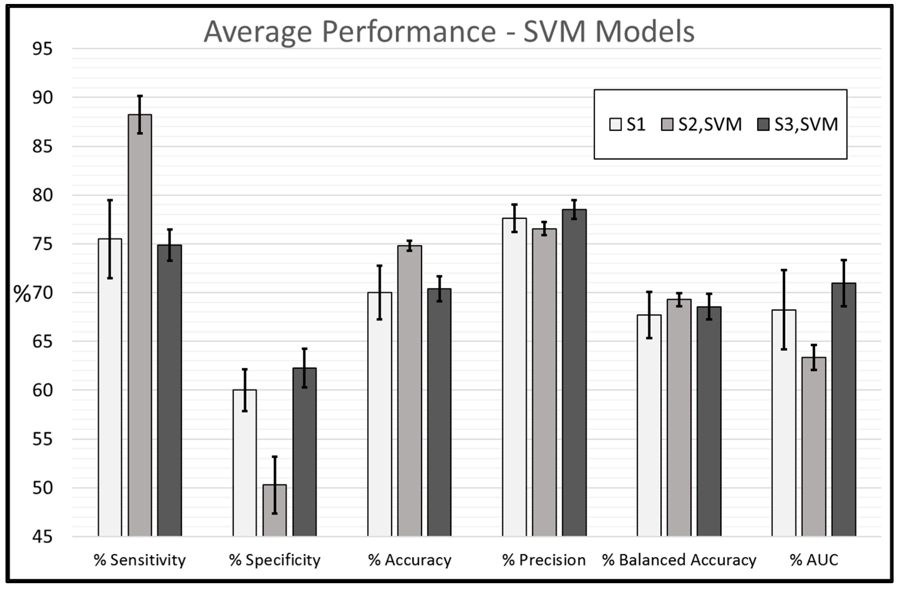
In summary, the results suggest that feature sets were enhanced by incorporating 2LTFs and 3LTFs for classifier training. The best performance for each classifier was the seven-feature multivariable model trained using S₃ feature sets. The seven-feature SVM classifier multivariable model had %S_n = 76%, %S_p = 64%, %Acc = 72%, %Prec = 80%, %Bal Acc = 70%, and AUC = 0.717, and the k-NN classifier model, %S_n = 74%, %S_p = 68%, %Acc = 72%, %Prec = 81, %Bal Acc = 71, and AUC = 0.700. Figure 4 and Figure 5 represent the average performance of all seven models trained using S₁, S₂, and S₃ feature sets for SVM and k-NN classifiers, respectively. To our knowledge, this is the first time DTA methodology has been investigated for CT scans.

4. Discussion

In this study, texture features determined from treatment-planning CT scans of H&N cancer patients yielded phenotypic insights regarding treatment endpoints. Pre-treatment GLCM, GLDM, GLRLM, and GLSZM texture features (S₁) from treatment-targeted LNs proved useful in training SVM and k-NN ML classifiers for binary treatment outcome prediction. Feature selection was performed using SFS for models with 1–7 features. For SVM classifier models, the best balanced accuracy was found with a six-feature multivariable model with %S_n = 78.3%, %S_p = 64, %Acc = 73.2, %Prec = 80.0, %Bal Acc = 71.1, and AUC = 0.651. The six selected features were “GLSZM Gray Level Variance”, “GLDM Small Dependence Emphasis”, “GLSZM Zone Percentage”, “GLCM Informational Measure of Correlation 1 (IMC1)”, “GLCM Inverse Difference Normalized (IDN)”, and “GLCM Inverse Difference Moment (IDM)”, the first five of which were computed as feature maps for 2LTF determination. “GLSZM Gray Level Variance” is a Pyradiomics feature that measures the variance in gray level intensities for the ‘zones’ within the GLSZM [33]. A gray level ‘zone’ is defined as the number of connected voxels (or pixels) that share the same gray level intensity [33]. Therefore, identification of GLSZM Gray Level Variance supports the notion that ROI heterogeneity impacts treatment efficacy. The next feature was “GLDM Small Dependence Emphasis”, which is a measure of the distribution of small dependencies, with a greater value indicative of smaller dependence and less homogeneous textures [33]. A “dependency” in regard to GLDM is the number of connected voxels (or pixels) within a specific distance and magnitude that are dependent on a central voxel [33]. The next feature was “GLSZM Zone Percentage”, which measures the coarseness of the texture by taking the ratio of the number of zones and the number of voxels in the ROI. The remaining three features, “GLCM IMC1”, “GLCM IDN” and “GLCM IDM”, are various methods of quantifying texture heterogeneity.

Similarly, for the k-NN classifier models, the highest multivariable model balanced accuracy came from the six-feature model with %S_n = 69.5%, %S_p = 68%, %Acc = 69%, %Prec = 80%, %Bal Acc = 68.8%, and AUC = 0.664. The six selected features were “GLDM Gray Level Non-Uniformity”, “GLSZM High Gray Level Zone Emphasis”, “GLRLM Gray Level Non-Uniformity”, “GLRLM Run Length Non-Uniformity Normalized”, “GLCM Joint Entropy”, and “GLSZM Gray Level Non-Uniformity”, the first five of which were made into feature maps for 2LTF determination. “GLDM Gray Level Non-Uniformity” measures the similarity of gray-level intensity values in the image, with lower values correlating with greater similarity in intensity values [33]. Quantifying “similarity” in pixel intensities within the ROI can be thought of as analogous to measuring homogeneity. The next three features, “GLSZM High Gray Level Zone Emphasis”, “GLRLM Gray Level Non-Uniformity”, and “GLRLM Run Length Non-Uniformity”, are all measures of heterogeneity within the ROI [33]. The final selected feature that was used to determine 2LTFs was “GLCM Joint Entropy”, which measures the randomness or variability in the neighbourhood intensity values within the GLCM.

Predicting biological endpoints with radiomics features is a growing area of research. For example, Tang et al. reported contrast-enhanced CT radiomics features acquired pre-treatment to be useful in predicting recurrence within two years of locally advanced esophageal SCC with radiomics features alone, clinical features alone, and combined clinical (7 features) and radiomics features (10 features), with %S_n = 87%, 79%, and 89% respectively (n = 220) [27]. Another study by Huang et al. reports success in predicting metastasis and extranodal extension in H&N patients with preoperative CT-scan radiomics features, even when compared to experienced radiologists (n = 464) [39]. For predicting metastasis, Huang et al. found %Acc = 73.8% for radiologist performances and %Acc = 77.5% for model performance [39]. For predicting extranodal extension, radiologists performed with %Acc = 70.4%, whereas the model performed with %Acc = 80% [39].

Radiomics studies are not limited to features determined from CT images. For example, for the prediction of preoperative cavernous sinus invasion from pituitary adenomas, a condition of interest for determining optimal treatment planning, radiomics features evaluated from contrast-enhanced T₁ MRI scans were used to train a linear support vector machine model with %Acc = 80.4%, %S_n = 80.0%, %S_p = 80.7%, and AUC = 0.826 [40]. In another study, MRI radiomics were investigated to differentiate between low-grade glioma and glioblastoma peritumoral regions [41], and yet another investigated prediction of response to neoadjuvant chemotherapy in patients with locally advanced breast cancer.

Previously, the DTA method was investigated for the first two layers for QUS texture features determined from LN quantitative ultrasound parametric maps, for the same cohort of patients [24]. DTA methodology and the inclusion of 2LTFs improved model performance in the QUS study as well (seven-feature SVM model %S_n = 81% improved to %S_n = 85%, %S_p = 76% improved to %S_p = 80%, %Acc = 79% improved to %Acc = 83%, %Prec = 86% improved to %Prec = 89%, and AUC increased from 0.82 to 0.85) [24]. Overall, models trained using QUS features outperformed the models in that study, suggesting that they reveal more phenotypic insight regarding treatment efficacy. This could be due to the fact that in the QUS study, features were determined from QUS parametric maps, ultrasound parameters known to be associated with tissue microstructures [42], whereas, in this study, features were determined from the CT image itself. Most importantly, however, both studies confirm that the inclusion of deeper layer texture features through the DTA methodology can improve model training.

However, it should be noted that radiomics studies do not always yield effective predictive capabilities, as was reported by Keek et al. who investigated radiomics features (GLCM, GLRLM, and GLSZM features in addition to first-order and shape features) from H&N SCC for prediction of overall survival, locoregional recurrence, and distant metastasis after concurrent chemo-radiotherapy (n = 444), using Cox proportional hazards regression and random survival forest models, and found that radiomics features from the peritumoral regions are not useful for the prediction of time to overall survival, locoregional recurrence, and/or distant metastasis, which the authors posit may be related to high variability between training and validation datasets [43]. Another study (with a large cohort (n = 726)) by Ger et al. found that prediction of overall survival did not improve after incorporating radiomics features, which was concluded when comparing a model trained using HPV status, tumour volume, and two radiomics features to a model using just tumour volume alone, and found that the AUC of the radiomics-included model was lower than the AUC of the model with tumour volume alone; however, the authors did comment on the potential advantages of using LN radiomics features instead of primary tumour features [44].

Furthermore, deeper layer texture features were determined only for feature maps made from top-five selected features from previously trained models. One could, hypothetically, create feature maps for every feature and subsequently acquire deeper layer textures for all available features before any model building; however, the proposed method of initial model building and feature selection makes sense not only intuitively, but also practically. For example, consider that in this work, the S₁ dataset included 70 (24 GLCM, 16 GLRLM, 16 GLDM, and 14 GLSZM) 1LTFs. If feature maps were made from all 70 features and 2LTFs were determined for all 70 feature maps, the subsequent S₂ dataset would include 4970 features (70 1LTFs + 4900 2LTFs). If the same process was repeated to incorporate 3LTFs, S₃ would include >300,000 features. However, through model building and feature selection at each layer, only important features are highlighted and “zoomed in” on or “focused on” through deep texture analysis. The calculation of textural features from the LN ROIs ranged in the order of minutes, whereas the computational time to create the texture feature maps ranged from a few hours to a few days depending on the complexity of the calculation, size of ROI, and quantization of pixel intensities. In this study, the number of features was greater than the number of samples, which means we had an underdetermined equation system. In this situation, the probability of overfitting is considerably high. To circumvent this challenge, we applied feature selection to reduce the dimension of data.

Although the results were promising, it should be noted that due to a small sample size, these models are not yet generalizable for clinical applications. Moreover, patients in this study were recruited with the presence of bulky neck disease, which represents a subset of all H&N cancer patients. However, the utility of this work may be clinically useful since it is exactly such patients with bulky disease who typically respond poorly to treatment and can benefit from adaptive radiotherapy in the future with response-predictive input on the basis of imaging. Furthermore, predictive models could incorporate clinical features, such as smoking and drinking history, along with HPV status, in model training. In this work, the feasibility of radiomics features was evaluated, and in particular, the influence of 2LTFs and 3LTFs was investigated. Further, features could be determined from the primary tumour as well as the LNs; however, in this study, some patients had unknown primary tumours. Additionally, with the understanding that cancerous cells extend beyond the visible GTV margins, some radiomics studies also evaluate features from the tumour margins [45]. Despite the limitations, the results in this study were promising, suggesting that treatment response can be predicted from treatment-planning CT scans and associated LN segmentations. Additionally, it seems that DTA methodology enhanced the quality of feature sets, and these results were consistent with previous work on QUS features for the same patient cohort. In the future, texture features and, in particular, the proposed DTA methodology will be investigated for the same patient cohort, using features determined from diagnostic contrast-enhanced T₁ MRI scans. Finally, an investigation will be performed to compare models trained using features from each of the three modalities, as well as training models on a combination of QUS + CT + MRI features.

Lastly, it is worth bringing attention to the fact that as an alternative to determining radiomics features and model building, another approach could be to utilize deep learning methods to build models directly from the images. Huynh et al. investigated the effectiveness of predictive models using conventional radiomics features with deep learning models and found that CNNs trained on images achieved the highest performance and that adding radiomics and clinical features to these models could enhance the performance further [46]. When testing models with radiomics and clinical features, it was found that they were susceptible to overfitting and, in particular, poor cross-institutional generalizability perhaps due to small sample sizes and variability in data procuring [46]. However, although deep learning approaches yield attractive results, they can be considered as “black boxes” with limited transparency and interpretability. The potential for radiomics models is in the fact that the features are well defined, and identification of important radiomics features with respect to any biological endpoint allows for further study and physiological investigation, in an effort to better understand the nature of the condition in question.

5. Conclusions

This study was designed based on the hypothesis that the index LNs of H&N cancer patients contain radiological phenotypes that can be correlated to and prove insightful in predicting the treatment response of the primary tumour and nodal disease. With modern healthcare approaches centered on personalized medical care, reliable and generalizable predictive models would provide clinicians with yet another tool in the treatment-planning protocol. Predictive models would benefit both CR and PR patients in better understanding their potential treatment outcomes, which can assist them in their decision making. Finally, it was found that DTA methodology and deep layer texture features can enhance predictive model performance and are worth consideration in future radiomics studies going forward.