Communication

Proposed Framework for Comparison of Continuous Probabilistic Genotyping Systems amongst Different Laboratories

1
Centre for Forensic Science, School of Mathematical & Physical Sciences, Faculty of Science, University of Technology Sydney, Ultimo, NSW 2007, Australia
2
Centre for Genomics and Personalised Health, Genomics Research Centre, School of Biomedical Sciences, Institute of Health and Biomedical Innovation, Queensland University of Technology, Brisbane City, QLD 4000, Australia
3
Department of Justice Studies, San Jose State University, San Jose, CA 95192, USA
4
The Forensic Institute, Glasgow G1 2LW, UK
5
School of Environment and Science, Griffith University, Nathan, QLD 4111, Australia
*
Author to whom correspondence should be addressed.
Submission received: 31 March 2021 / Revised: 27 May 2021 / Accepted: 3 June 2021 / Published: 10 June 2021

Abstract

:
Continuous probabilistic genotyping (PG) systems are becoming the default method for calculating likelihood ratios (LRs) for competing propositions about DNA mixtures. Calculation of the LR relies on numerical methods and simultaneous probabilistic simulations of multiple variables rather than on analytical solutions alone. Some also require modelling of individual laboratory processes that give rise to electropherogram artefacts and peak height variance. For these reasons, it has been argued that any LR produced by continuous PG is unique and cannot be compared with another. We challenge this assumption and demonstrate that there are a set of conditions defining specific DNA mixtures which can produce an aspirational LR and thereby provide a measure of reproducibility for DNA profiling systems incorporating PG. Such DNA mixtures could serve as the basis for inter-laboratory comparisons, even when different STR amplification kits are employed. We propose a procedure for an inter-laboratory comparison consistent with these conditions.

1. Introduction

As forensic short tandem repeat (STR) genotyping assays have become more sensitive, DNA samples that may once have been classified as single source (assessed as being derived from a single DNA donor) may instead be classified as having multiple contributors as low-level alleles are now detected. The presence of multiple contributors has significant implications for propositions involving DNA transfer, persistence, prevalence and recovery (TPPR) [1]. Estimating the weight of evidence of these mixtures with the combined probability of inclusion/exclusion (CPI/E) has proved limiting, mostly because of problems with the treatment of allele drop in and drop out [2,3,4]. As a result, in many jurisdictions, probabilistic genotyping (PG) has become the default process for generating likelihood ratios (LRs) for forensic analysis of DNA mixtures [5]. Continuous PG algorithms model the probability distributions of observed peak heights in STR electropherograms (epgs) under different scenarios. These can then be used to generate likelihoods for propositions which can in turn be combined into LRs. There are a number of continuous PG algorithms available including DNA·VIEW® [6], TrueAllele® Casework [7,8] (Cybergenetics, Pittsburgh, PA, USA), STRmix™ [9] (Institute of Environmental Science and Research, Forensic Science South Australia, Adelaide, SA, Australia), EuroForMix [10] and DNAxs [11]. The latter two PG systems are an extended version of the model proposed by Cowell et al. [12] which is open source while the other three require commercial licences [13,14,15]. Until relatively recently [16], there has been little evidence that continuous PG is reproducible amongst different laboratories, and little attempt has been made to define credible intervals for the LRs produced.
Swaminathan et al. [17] collated the LRs for 30 × one-person samples, 82 × two-person mixtures and 90 × three-person mixtures generated by four variations of their CEESIt continuous PG algorithm [18]. The four variations included different permutations of models for “mixture ratio” (also known as the “mixture proportion” [19] and as a “mass parameter” [9,20]), peak height distribution and forward stutter designed to mimic the diversity of available continuous PG algorithms. LRs were calculated five times for each mixture to assess intra-model variance resulting from the Markov chain Monte Carlo (MCMC) simulation procedure. In all four models, intra-model variability increased with an increase in the number of contributors and with a decrease in the contributors’ template mass. The LRs were binned into ranges corresponding with verbal expressions for the weight of evidence according to the Association of Forensic Science Providers [21] ranging from “weak” for an LR between 1 and 10 to “extremely strong” for an LR > 106. For 9% of intra-model comparisons, LRs did not fall in the same bin for the same mixture, and for 1.5%, LRs were more than one bin apart. For 16% of inter-model comparisons (where two or more of the four models yielded LRs in the same bin for all five runs), LRs from one model fell in a different bin from one or more other models, and 11% were more than one bin apart.
Bright et al. [22] originally proposed and demonstrated a series of tests for validating PG systems using single source, simulated major/minor (3:1) mixtures and simulated balanced (1:1) mixtures. The LRs generated by PG were compared with those expected under theoretical modelling in Excel. Input electropherograms had peak heights adjusted so that there was:
  • No possibility of drop in and drop out;
  • No possibility of drop in but some possibility of drop out;
  • No possibility of drop out but with artificial alleles added to mimic the possibility of drop in.
Replicate analyses were employed to test for reproducibility. The results of their tests showed good agreement between expected results, continuous PG and semicontinuous PG for single source and balanced profiles, although for the latter, continuous PG yielded higher LRs than semicontinuous PG, as expected. This is because of the extra peak height information considered by continuous PG. For major/minor profiles, agreement between continuous and semicontinuous PG only occurred when the major contributor was manually extracted. This is because continuous PG is able to take advantage of the peak height information in an unbalanced mixture while semicontinuous PG does not (putting aside manual interpretation by an analyst of stutter peaks, for example). All electropherograms were simulated from single source profiles derived from the same capillary electrophoresis instrument, and only one continuous PG algorithm (STRmix) was employed.
There have been other attempts to compare the reproducibility of outputs amongst different PG systems, but most of these (e.g., [23,24,25,26,27]) have involved submitting the same epgs from the same STR amplification kits to different PG algorithms. Benschop et al. [28] describe a validation of one PG system (DNAxs) in five laboratories using STR genotype data (alleles and peak heights) generated within each laboratory from different STR assays. Each laboratory shared its genotyping results with the others, and LRs were mostly within an order of magnitude for the same genotype data. However, the same DNA samples were not processed in each individual laboratory so that the LRs were all generated from the same epgs. Alladio et al. [29] showed that it was possible to compare the reproducibility of LRs from different PG systems and different STR assays. The LRs generated from DNA·VIEW, STRmix and EuroForMix were reproducible for high DNA template amounts over a wide range of mixtures with different numbers of contributors and mixture ratios. Once again, the LRs were all generated from the same epgs. Different STR assays produced LRs that differed by many orders of magnitude, as expected. This is because different STR assays employ different STR loci and different numbers of loci. While this might seem like an impediment to inter-laboratory comparisons, we demonstrate that it can be overcome.
Inter-laboratory comparisons are a standard feature of forensic DNA analysis methods [16,26,30,31,32]. They indicate the reproducibility of a particular method amongst different laboratories and the variance of quantitative results. It is a reasonable expectation that they be undertaken. They serve to calibrate amongst laboratories, which helps to ensure equality of justice outcomes amongst jurisdictions. The US President’s Council of Advisors on Science and Technology (PCAST) “believes that test-blind proficiency testing of forensic examiners should be vigorously pursued, with the expectation that it should be in wide use, at least in large laboratories” [33]. The US National Institute of Standards and Technology (NIST) states: “Inter-laboratory tests are the means by which multiple laboratories compare results and demonstrate that the methods used in one’s own laboratory are reproducible in another laboratory. These tests are essential to demonstrate consistency in results from multiple laboratories” (quoted from [34]).
McNevin et al. [35] have previously suggested a method for assessing reproducibility and defining credible intervals for LRs derived from the same DNA extracts (not electropherograms) and calculated by STRmix in particular and continuous PG in general. This was met with some scepticism by Buckleton et al. [36] who contend, firstly, that there are “multiple reasonable answers in the case of evidence from one extract” [36,37] and, secondly, that it is sufficient to calibrate the LRs generated by PG from multiple laboratories using the method of Ramos and Gonzalez-Rodriguez [38]. In summary, this last method uses the LRs and a prior odds ratio from known numbers of contributors and non-contributors submitted by multiple laboratories to calculate a posterior odds ratio. The posterior ratio is compared with the relative frequencies of contributors. The number of non-contributors with LR above a certain threshold should reflect the number expected given the numbers of contributors and non-contributors [39]. This is a reasonable test of the bulk or macro properties of the LR from multiple laboratories; however, it does not provide any indication of the variance in LRs amongst laboratories for the same sample or whether an individual laboratory is producing reasonable LRs. For example, in a multi-laboratory comparison, a laboratory that consistently produces large LRs might be balanced by a laboratory that consistently produces small LRs without perturbing the bulk or macro properties of all the LRs produced. It also requires a large number of contributors and non-contributors for many mixtures.
We argue that there is a true test of each laboratory’s ability to produce reasonable LRs, consistent with McNevin et al. [35] and regardless of the instrumentation and STR assays used to produce epgs. Here we provide a formal proof that such a test exists, and we define the conditions under which such a test could be performed.

2. The Likelihood Ratio Produced by Probabilistic Genotyping

We start with the general formulation of the LR for a DNA mixture as a ratio of two conditional probabilities:
LR = P ( E | H 1 ) P ( E | H 2 )
We will loosely follow the notation of Taylor, Bright and Buckleton [9,20] in their descriptions of PG systems while acknowledging that other notations exist (e.g., [12,19]). The evidence, E, is an electropherogram (epg) from a crime trace (GC) exhibiting a mixture of known reference profiles (GR) and unknown profiles (GU). There is also a person or persons of interest (POI or POIs). In general, one proposition, H1, is that a particular reference genotype (or genotypes) from a POI or POIs (GP) is a contributor to the DNA mixture, while the alternate proposition, H2, is that the contributors are two or more known (GR) or unknown (GU) genotypes not including the POI(s). The propositions can take various forms, but H2 will always differ from H1 in that the genotype of at least one POI (GP) is replaced with an unknown genotype (GU), for example:
H 1 = { G P , G R 1 , G R 2 , G R 3 ,   ,   G U 1 , G U 2 , G U 3 ,   }
H 2 = { G R 1 , G R 2 , G R 3 ,   ,   G U 0 , G U 1 , G U 2 , G U 3 ,   }
Cowell et al. [12] show that, under the assumption of Hardy–Weinberg equilibrium (HWE), the LR for a mixture for which GP in H1 is replaced by an unknown profile (GU0) in H2 can never be greater than the LR for a single source profile for the POI responsible for GP. This places an upper limit on the LR under these circumstances.
The epg reveals M genotype sets S of possible explanatory genotype combinations from N contributors that could give rise to the DNA mixture at any locus. The likelihood ratio becomes:
LR = m = 1 M p ( G C | S m ) P ( S m | H 1 ) m = 1 M p ( G C | S m ) P ( S m | H 2 )
where Sm is the mth possible explanatory genotype combination for N contributors and p(GC|Sm) is a conditional probability density (distinguishing it from a point probability, P). As an example, consider an epg at a locus where there are four alleles (A, B, C, D) detected above an analytical threshold. Possible genotype sets for two presumed contributors include {AB, CD}, {AC, BD}, {AD, BC}. There may also be genotype sets that do not include all detected alleles, for example, {BC, BD}, {BC, CD}, {BD, CD}, {BB, CD}, {BD, CC}, {BC, DD}, with A as an artefact (e.g., drop in or stutter). For three presumed contributors, possible genotype sets include {AA, BB, CD}, {AA, BC, DD}, {AB, CC, DD}, etc. There may also be genotype sets that include undetected alleles, for example {AB, CD, AE}, {AB, CD, BE}, {AB, CD, CE}, {AB, CD, DE}, etc, with E as a drop out. A “weight”, wm, can be used to describe the conditional probability density for observing the mixture profile given Sm:
w m = p ( G C | S m )
where:
m = 1 M w m = 1
The normalised weights vary from 0 to 1 and account for the possibilities of allele drop in and allele drop out. For continuous PG, they also account for the possibilities of stutter, peak height stochasticity, peak height degradation and peak height variations as a result of allele overlap (shared alleles). Semicontinuous PG does not consider peak height information, although stutter must be differentiated from true alleles by the analyst. The weights for continuous PG are modelled using what Taylor et al. [9,20] refer to as “mass parameters” including a template DNA amount for each contributor, a degradation level for each contributor, an assay-specific locus amplification efficiency for each locus and a replicate amplification efficiency for each replicate. The last two parameters account for inter-locus and inter-replicate variabilities, respectively. The likelihood ratio then becomes:
LR = m = 1 M w m P ( S m | H 1 ) m = 1 M w m P ( S m | H 2 )

3. A Reproducible Subset of Likelihood Ratios from Probabilistic Genotyping

The values for wm will vary from laboratory to laboratory. This is because each laboratory must model epg artefacts and peak height variance for the particular conditions in their laboratory, and these models inform the various w. At first glance, and this is certainly the view of Buckleton et al. [36], this suggests that LRs reported by different laboratories cannot be compared. While it is true that not all LRs can be compared, we can define specific conditions for which a subset of LRs can be compared. These conditions exist when the values of wm are the same for different laboratories.
The weight or likelihood, wm, for any genotype set, Sm, will vary from almost impossibility (wm  0) to almost certainty (wm  1). We distinguish between genotype sets with at least one allele not belonging to any of the contributors or without all contributor alleles present (Si) and those with all alleles belonging to contributors and no others (Sj):
LR = i w i P ( S i | H 1 ) + j w j P ( S j | H 1 ) i w i P ( S i | H 2 ) + j w j P ( S j | H 2 )
For our four-allele example, let us assume that the contributors have genotypes BC and CD (A is an artefact). Genotype sets Si include any genotypes with allele A (AA, AB, AC, AD) or without at least one of B, C and D, while genotype sets Sj include all of B, C and D but not A (or any undetected alleles). We wish to restrict wi so that each laboratory finds wi  0. Under these conditions, for any PG system:
lim w i 0 LR = j w j P ( S j | H 1 ) j w j P ( S j | H 2 )
We then extract the unique genotype set S * that corresponds with the contributors to the mixture:
lim w i 0 LR = k w k P ( S k | H 1 ) + w * P ( S * | H 1 ) k w k P ( S k | H 2 ) + w * P ( S * | H 2 )
where w * is the weight assigned to S * and the new subscript k is used because S * has been separated from the other Sj. For our four-allele example, S * is {BC, CD} which is now distinguished from {BC, BD}, {BD, CD}, {BB, CD}, {BD, CC}, {BC, DD}, etc. When H1 corresponds with the contributors only (H1 true) then P ( S k | H 1 ) = 0 , P ( S * | H 1 ) = 1 and:
lim w i 0 LR = w * k w k P ( S k | H 2 ) + w * P ( S * | H 2 ) 1 P ( S * | H 2 )
Note that there is an upper limit for LR which occurs if all wk  0. This is essentially the same result obtained by Cowell et al. [12] for continuous PG but generalised for multiple contributors. When H1 corresponds with non-contributors (H1 false) where at least one allele of a non-contributor is not shared with a true contributor then P ( S k | H 1 ) 0 , P ( S * | H 1 ) 0 and LR 0.
For semicontinuous PG, we have no way to reduce uncertainty amongst Sk and S * (because peak height information is not considered). All remaining genotype sets are equally likely. Hence, w * = w k = w . In this case, Equation (8) becomes:
lim w i 0 LR = w k P ( S k | H 1 ) + w P ( S * | H 1 ) w k P ( S k | H 2 ) + w P ( S * | H 2 ) = k P ( S k | H 1 ) + P ( S * | H 1 ) k P ( S k | H 2 ) + P ( S * | H 2 )
When H1 corresponds with the contributors only (H1 true):
lim w i 0 LR = 1 k P ( S k | H 2 ) + P ( S * | H 2 )
This is the minimum performance expected of continuous PG. We therefore have an upper and lower bound for the LR from continuous PG if:
  • wi  0 (i.e., uncertainty is minimised between genotype sets with all alleles belonging to contributors and no others and those with at least one allele not belonging to contributors or without all contributor alleles present) and;
  • H1 is true (i.e., H1 corresponds with the contributors only).
The range of expected values is given by:
1 k P ( S k | H 2 ) + P ( S * | H 2 ) < lim w i 0 LR < 1 P ( S * | H 2 )
The lower bound is the LR for the same mixture derived from semicontinuous PG, and the upper, aspirational bound is the LR that would be possible if uncertainty could be eliminated amongst the true contributor genotype set, S * , and all others. To move from the lower bound to the upper bound requires increasing w * beyond the average weight used for semicontinuous PG. Indeed, this is the goal of continuous PG, and the relative ability to increase w * over all other weights is a performance measure for continuous PG systems.

4. Conditions for Achieving Reproducible LRs from Probabilistic Genotyping

The conditional probabilities, P ( S * | H 1 ) and P ( S * | H 2 ) are match probabilities defined by true contributor reference profiles, population genetic models, population allele frequencies and two alternative propositions. As long as any two laboratories have reference profiles for the same contributors, consider the same propositions and use the same models (e.g., Hardy–Weinberg proportions, NRC II recommendation 4.1, NRC II recommendation 4.2), the same population allele frequencies and the same θ for the same loci, they should obtain the same values for P ( S * | H 1 ) and P ( S * | H 2 ) . This defines our first conditions for an inter-laboratory comparison of LRs:
  • The same standard mixtures should be examined.
  • The same propositions should be considered.
  • The same loci should be employed.
  • The same population allele frequencies should be employed.
  • The same population genetic model and sub-structure correction, θ, should be employed (e.g., θ = 0).
Satisfying Equation (7) requires reducing the probabilities of genotype sets with at least one allele not belonging to any of the contributors or those without all contributor alleles present such that wi  0. This will occur when there is little uncertainty between:
  • No allele and allele drop out;
  • A (low peak height) contributor allele and allele drop in;
  • A (low peak height) contributor allele and a stutter peak;
  • A single allele and shared (“stacked”) alleles, either of which may or may not include allele drop in and stutter peaks.
We consider each of these in turn.
The greater the amount of contributor DNA in the mixture, the higher contributor allele peaks are likely to be. The higher the allele peaks, the less likely that drop out will occur. Similarly, high allele peaks are unlikely to be confused with (low peak height) allele drop in. Stochastic variation in peak heights will also be minimised with increasing peak height. Heterozygote peak height imbalance has been shown to decrease as average peak height (APH) increases [40,41]. Continuous PG algorithms model allele peak height and stutter peak height to reflect observations that variance decreases with peak height. EuroForMix and TrueAllele use gamma [10] and normal distributions [7], respectively. STRmix models allele peak and stutter peak height variation according to a log normal distribution [9,20,42]:
log 10 ( O a E a ) ~ N ( 0 , c 2 E a )
log 10 ( O a 1 E a 1 ) ~ N ( 0 , k 2 O a )
O and E refer to observed and expected peak heights for alleles (a) and stutter (a − 1), and c2 and k2 are locus-specific random variables which are in turn modelled by gamma distributions. For both allele and stutter peaks, the variance is inversely related to peak height (Ea and Oa, respectively) such that stochastic variation will be reduced with increasing peak height.
Too much DNA, however, will result in overloading of the epg with split peaks, pull ups and other artefacts, after which true allele peaks can be confused with these artefacts. This provides our next condition for an inter-laboratory comparison of LRs:
6.
The DNA template from true donors should be maximised to a point within the linear range and below saturation of the epg.
The optimal amount of DNA defined by condition 6 may be difficult to assess. One way to achieve it is to amplify a dilution series of DNA such that there is a range of DNA template input amounts ranging from below the optimum to above the optimum. This is a general approach when assessing PG systems (e.g., [41,43,44]) and has been previously used to compare amongst them [29]. The LR will approach a maximum for H1 true as DNA template amount increases and as wi  0. This is demonstrated by Bauer et al. [44] in their Figure 1 (originally in [8]) and defines our next condition:
7.
Each laboratory is presented with aliquots of the same dilution series of DNA solutions which then undergo analyses to produce epgs for each solution according to each laboratory’s standard practice (according to which the PG system was validated in that laboratory).
Stutter artefact peak heights will scale with true allele peak heights approximately according to a stutter ratio. Hence, conditions 6 and 7 are insufficient on their own to reduce uncertainty between stutter peaks and smaller true allele peaks. Similarly, they will not reduce uncertainty between single alleles and stacked alleles. If the contributors to a DNA mixture are present in equal proportion, however, this uncertainty is minimised, and different labs and different PG systems will tend to find the same wj. Cheng et al. [45] have recently demonstrated that peak heights are additive and proportional to the donor contributions in a DNA mixture epg. This means that if an allele is shared by two donors, then it should have double the height expected from an allele belonging to a single donor if both donors’ DNA templates are not degraded and are present in equal proportion. If it is shared by three donors, it should have triple the height expected from an allele belonging to a single donor if all three donors’ DNA is present in equal proportion, and so on.
Stutter peak heights are typically 15% or less of the parent allele peak height, depending on the length of the longest uninterrupted repeat chain [46]. Uncertainty between a stutter peak and a true allele will occur if one contributor is present in the mixture with this order of magnitude relative to another donor (15% or less). When all contributors to a mixture are present in equal proportion, then the size of each donor’s allele peak should be approximately 100% relative to all other donors’ peaks (albeit with stochastic variance and taking account of degradation) and thus less likely to be confused with a stutter peak. Our next condition for an inter-laboratory comparison of LRs is:
8.
All known donors are present in equal proportion by DNA template amount.
We now have the eight conditions for an inter-laboratory comparison originally suggested by McNevin et al. [35]. Such a comparison should produce the results described by them in their Figure 1 and by Bauer et al. [44] in their Figure 1 where the maximised value of the LR corresponding with the plateau in both cases is given by Equation (7) for all propositions and Equation (9) for H1 true (Figure 1). We would go so far as to say that Equation (12) defines the “expected” LR range under our eight conditions, in the same way that the reciprocal of the random match probability is the expected LR for a high quality single source profile. We acknowledge that there is debate here, including a special issue in Science & Justice devoted entirely to measuring (or not) the reproducibility of LRs [47], but the upper bound for the LR defined in Equation (9) is certainly aspirational.
We add two final conditions that should be employed for any inter-laboratory comparison consistent with best scientific practice. These are:
 9.
The trial should be blinded. Laboratories presented with a dilution series of DNA solutions to be analysed should not know which is which.
10.
The trial should be facilitated by an entity not associated with the PG systems under comparison.
LR > 1 from semicontinuous PG will nearly always be less than the LR from continuous PG for the same mixture for H1 true, except at low DNA template amounts when stochastic effects dominate. This is because more information (peak heights) is being used by continuous PG resulting in LRs further from 1. Exceptions may occur when a sample has an unlikely peak height that greatly deviates from the expected height, possibly due to extreme stochastic variation or a primer sequence polymorphism (null allele). This can lead to very low weights for S * and thus a lower LR than for semicontinuous PG. Such exceptions notwithstanding, Equation (12) defines a theoretical range for the LR from continuous PG where the lower bound is the LR from semicontinuous PG and the upper bound represents no uncertainty amongst the true contributor genotype set, S * , and all others. The greater the number of equal-proportion contributors, the lower the LR and the lower the theoretical range defined by Equation (12) will be. This is because there are greater numbers of allele permutations that could explain contributor genotype sets, Sj, and hence the weight, wj, assigned to each one is lower.
We now address the questions of peak height imbalance and degradation (the typical “ski slope” of DNA profiles). STRmix (and, indirectly, other continuous PG systems) model these phenomena using the so-called mass parameters and then assign wm according to how far the observed peaks deviate from the modelled peaks. Allele decay is modelled as a function of molecular weight where longer alleles will have lower peak heights than shorter alleles. Different manufacturers of forensic STR assays will have different amplicon sizes for each of the loci and so the relative decay amongst loci will vary. At any particular locus, there will also be allele-specific variation leading to heterozygote imbalance, for example. For STRmix, this is modelled by Equations (13) and (14). If we consider two non-shared alleles in a genotype set, Sj, the further they are from equality (balanced), the lower the weight assigned to a heterozygous genotype in Sj, all other weights being equal.
Peak height variance and degradation have been posited by Buckleton et al. [36] as another reason LRs cannot be compared amongst laboratories. However, at any particular locus for any particular kit, we are restricting wm such that each laboratory finds wi  0 and wj are the same for all laboratories. A true heterozygous genotype may have two unbalanced and unshared alleles, but the heterozygous genotype will still have a much higher probability, wj, than other possible genotypes under our eight conditions, all other weights being equal.

5. An Inter-Laboratory Comparison

Our proposed conditions and trial will not provide a comparison point for every possible LR generated by continuous PG. This is because LRs produced by continuous PG are subject to variance. However, we have specified conditions that minimise this variance. Even less variance is possible if we specify conditions that minimise uncertainty between one POI and all other contributors (i.e., wi  0, wk  0, w *   1), but this is the trivial case where one contributor is present at much higher proportion than all others, approaching the case of a single source profile.
It may be argued that our set of conditions 1 to 8 is restrictive and does not test the reproducibility of PG systems when wi is not close to 0. However, by including a dilution series, we can see how the variance in LR increases from its minimum (at high average peak height, APH) as APH decreases. Swaminathan et al. [17] found that this variance increased with a decrease in the contributors’ template mass for all four of their representative continuous PG model variations. Conditions 1 to 8 therefore provide for a minimum performance measure. Our condition 8 is a strenuous test because, as Bucketon et al. [43] point out: “testing two low-level contributors with similar APHs (a 1:1 mixture) presents more of a challenge to the software than does a 1:20 mixture, as the genotype of the higher contributor has less uncertainty and helps to inform the genotype of the lower contributor”. This would equally be the case at high APHs.
An inter-laboratory comparison employing our conditions will provide the following information:
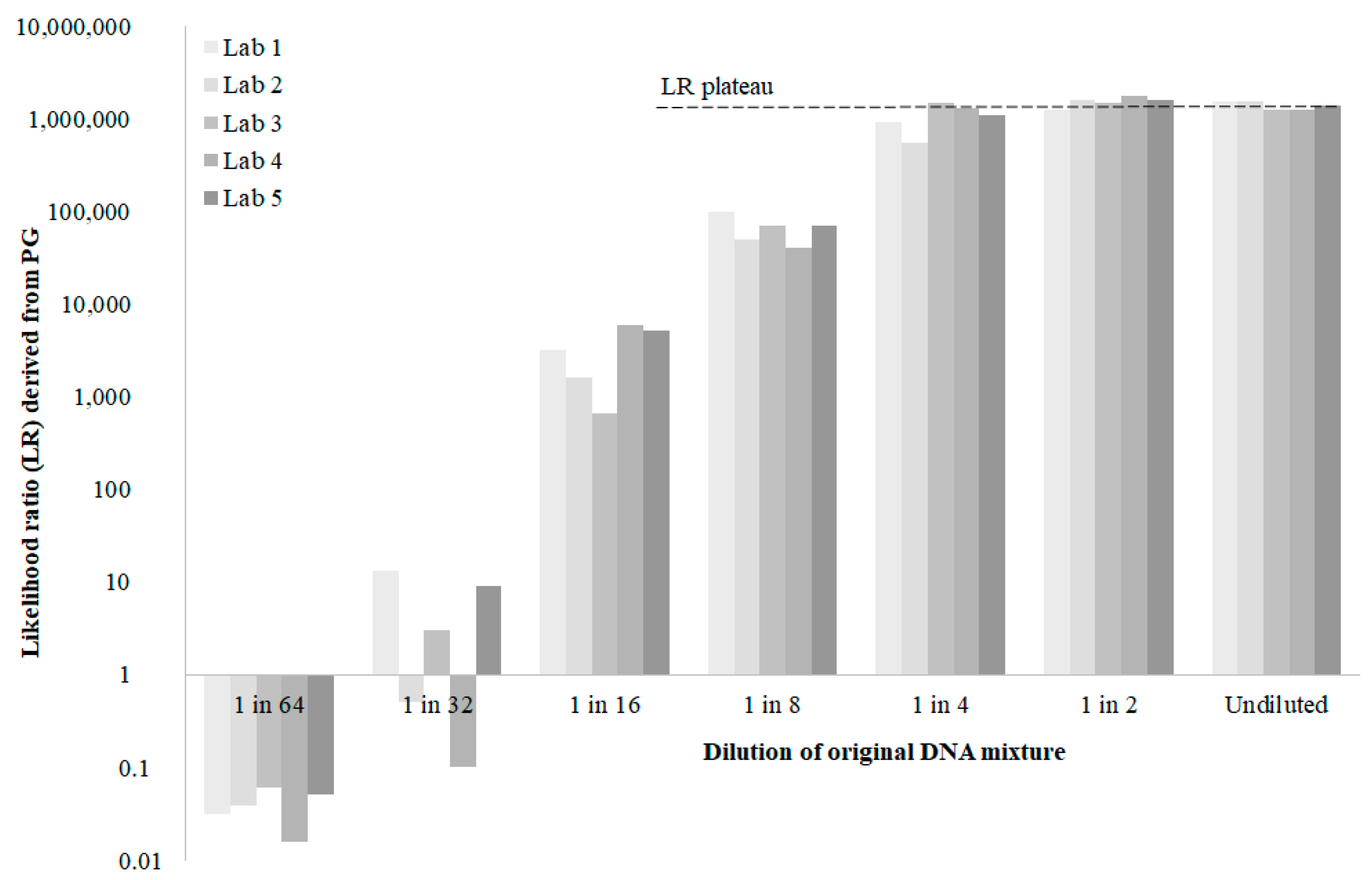
  • The position of the plateaued, maximum LR from any laboratory within the theoretical range defined by Equation (12). This is a measure of performance, if not accuracy.
  • The range of plateaued, maximum LRs reported by laboratories. This is an indication of the credible interval for LRs reported under the best possible conditions designed to minimise variance in LRs. This credible interval would suggest a minimum as we would expect the variance amongst laboratories to increase the further they are from conditions 1 to 8.
  • Outlier laboratories. This would provide guidance on which laboratories (if any) might need to re-validate their PG system.
  • Outlier PG systems. This would provide guidance on which PG systems (if any) do not model allele peak height variance adequately according to the procedures in a particular laboratory.
  • The minimum template amounts at which fortuitous LRs are encountered for any laboratory (LR > 1 for a non-contributor, LR < 1 for a contributor). As DNA template amounts decrease in the dilution series, LRs for contributors and non-contributors will approach 1 but may actually overshoot.
We now define the procedure for an inter-laboratory comparison consistent with our conditions 1 to 10:
  • Identify participating laboratories. They are required not to communicate with each other concerning the trial.
  • Identify reported loci in common amongst participating laboratories. Longer loci, where Equation (7) might not be expected to hold, could also be excluded (with agreement). These excluded loci should not be used either to estimate parameters such as mixture proportions or to calculate LRs. In practice, any laboratory could nominate a locus to be excluded. A comparison between PG systems could, theoretically, be made with as little as one locus but, of course, more loci will increase the stringency of any trial.
  • Identify a trial facilitator not associated with any of the PG systems to be used. This could be a university, a centre of excellence or a national forensic regulator, for example.
  • The trial facilitator collects samples from reference cell lines or consenting volunteers and performs DNA extraction and quantitation for each sample.
  • The DNA concentration for each sample is normalised according to the quantitation results and assessed as being of a suitable (high) quantity and quality.
  • A single source STR profile for each donor is generated according to best practice. These are the contributor reference profiles. Non-contributor reference profiles can also be generated.
  • Equal volume and equal concentration aliquots of high abundance DNA are combined from various donors to create mixtures of 2, 3, 4,… and N contributors in equal proportion by DNA amount.
  • For each mixture, a dilution series is created (e.g., undiluted, 1 in 2, 1 in 4, 1 in 8, etc.).
  • Aliquots of the various dilution series (one dilution series per mixture) are distributed to the participating laboratories, labelled randomly such that the laboratory does not know the concentration of DNA in any sample. For one, two, three, four and five contributors each at seven different dilutions, for example, a total of 35 samples would be supplied.
  • Each participating laboratory produces an STR epg for each aliquot according to the standard procedures for that laboratory.
  • The participating laboratories are also supplied with the following:
    • Reference profiles.
    • Allele frequencies from a defined population.
  • The following propositions are also provided to each of the participating laboratories:
    • H1: The donor of reference profile X is a contributor to the mixture which also consists of N other known but unrelated contributors (where all N+1 reference profiles are supplied);
    • H2: The donor of reference profile X is not a contributor to the mixture which consists of an unrelated, random member of the (defined) population and N other known but unrelated contributors.
    These can be applied to both contributor and non-contributor reference profiles.
  • Each laboratory is asked to provide a LR according to Equation (1). The laboratories are instructed to use the allele frequencies provided from the defined population without any population substructure corrections and using a consistent population genetic model (e.g., Hardy–Weinberg proportions).
  • The LRs are collated and compared by the trial facilitator.

6. Conclusions

We propose a procedure to allow comparison amongst PG systems and laboratories. The LR defined by Equation (7) and the LR range defined by Equation (12) and enabled by our conditions 1 to 8 will not depend on either the PG system or the laboratory if each PG system calculates LR according to Equation (5) and calculates wm according to maximum likelihood and if each laboratory has calibrated their PG system appropriately. Kelly et al. [40] state that LR “variance is more profile specific than laboratory specific” if c2 and k2 in Equations (13) and (14), respectively, are adequately modelled. Proposing that a PG system can be calibrated according to the procedures and instruments of a particular laboratory raises the question: Can that calibration be tested? We believe it can and that there is no reason to avoid inter-laboratory comparison of PG systems, even when different STR amplification kits are employed. Differences in STR assay, PCR thermal cycling, capillary electrophoresis or profile analysis settings will all be manifested in peak height variances which are modelled by PG systems. How well it is modelled will be determined by where any generated LR sits in the range defined by Equation (12) and, indeed, whether it falls in this range at all. We hope that our proposed study builds upon existing validation of continuous PG and provides another step towards establishing a standardised, best practice approach for DNA mixture analysis.

Author Contributions

Conceptualization, D.M., K.W. and J.C.; methodology, D.M., K.W., A.J. and J.C.; writing—original draft preparation, D.M.; writing—review and editing, K.W., M.B., S.G., A.J., J.C. All authors have read and agreed to the published version of the manuscript.

Funding

This research received no external funding.

Institutional Review Board Statement

Not applicable.

Informed Consent Statement

Not applicable.

Data Availability Statement

Not applicable.

Acknowledgments

The authors are grateful for feedback on various drafts from a number of individuals.

Conflicts of Interest

The authors declare no conflict of interest.

References

  1. van Oorschot, R.A.H.; Szkuta, B.; Meakin, G.E.; Kokshoorn, B.; Goray, M. DNA transfer in forensic science: A review. Forensic Sci. Int. Genet. 2019, 38, 140–166. [Google Scholar] [CrossRef]
  2. Perlin, M.W. Inclusion probability for DNA mixtures is a subjective one-sided match statistic unrelated to identification information. J. Pathol. Inf. 2015, 6, 59. [Google Scholar] [CrossRef]
  3. Bieber, F.R.; Buckleton, J.S.; Budowle, B.; Butler, J.M.; Coble, M.D. Evaluation of forensic DNA mixture evidence: Protocol for evaluation, interpretation, and statistical calculations using the combined probability of inclusion. BMC Genet. 2016, 17, 125. [Google Scholar] [CrossRef] [PubMed] [Green Version]
  4. Curran, J.M.; Buckleton, J. Inclusion probabilities and dropout. J. Forensic Sci. 2010, 55, 1171–1173. [Google Scholar] [CrossRef]
  5. Coble, M.D.; Bright, J.-A. Probabilistic genotyping software: An overview. Forensic Sci. Int. Genet. 2019, 38, 219–224. [Google Scholar] [CrossRef]
  6. Brenner, C.H. DNA·VIEW User’s Manual. Charles Brenner, UC Berkeley, 6801 Thornhill Drive Oakland, California, USA. 2019. Available online: http://dna-view.com/downloads/documents/manuals/DNAVIEW%202019%20US.pdf (accessed on 8 June 2021).
  7. Perlin, M.W.; Legler, M.M.; Spencer, C.E.; Smith, J.L.; Allan, W.P.; Belrose, J.L.; Duceman, B.W. Validating TrueAllele® DNA mixture interpretation. J. Forensic Sci. 2011, 56, 1430–1447. [Google Scholar] [CrossRef]
  8. Perlin, M.W.; Sinelnikov, A. An information gap in DNA evidence interpretation. PLoS ONE 2009, 4, e8327. [Google Scholar] [CrossRef] [PubMed]
  9. Taylor, D.; Bright, J.-A.; Buckleton, J. The interpretation of single source and mixed DNA profiles. Forensic Sci. Int. Genet. 2013, 7, 516–528. [Google Scholar] [CrossRef] [PubMed]
  10. Bleka, Ø.; Storvik, G.; Gill, P. EuroForMix: An open source software based on a continuous model to evaluate STR DNA profiles from a mixture of contributors with artefacts. Forensic Sci. Int. Genet. 2016, 21, 35–44. [Google Scholar] [CrossRef] [PubMed] [Green Version]
  11. Benschop, C.C.G.; Hoogenboom, J.; Hovers, P.; Slagter, M.; Kruise, D.; Parag, R.; Steensma, K.; Slooten, K.; Nagel, J.H.A.; Dieltjes, P.; et al. DNAxs/DNAStatistX: Development and validation of a software suite for the data management and probabilistic interpretation of DNA profiles. Forensic Sci. Int. Genet. 2019, 42, 81–89. [Google Scholar] [CrossRef]
  12. Cowell, R.G.; Graversen, T.; Lauritzen, S.L.; Mortera, J. Analysis of forensic DNA mixtures with artefacts. J. R. Stat. Soc. Ser. C 2015, 64, 1–48. [Google Scholar] [CrossRef] [Green Version]
  13. Get More Information from DNA Mixtures with TrueAllele® Casework. Available online: https://www.cybgen.com/products/casework.shtml (accessed on 16 May 2021).
  14. STRmix™. Empowering Forensic Science. Available online: https://www.strmix.com/ (accessed on 16 May 2021).
  15. Brenner, C. What is DNA•VIEW®? An Integrated Software Package for DNA Identification. Available online: http://dna-view.com/dnaview.htm (accessed on 16 May 2021).
  16. Butler, J.M.; Kline, M.C.; Coble, M.D. NIST interlaboratory studies involving DNA mixtures (MIX05 and MIX13): Variation observed and lessons learned. Forensic Sci. Int. Genet. 2018, 37, 81–94. [Google Scholar] [CrossRef] [PubMed] [Green Version]
  17. Swaminathan, H.; Qureshi, M.O.; Grgicak, C.M.; Duffy, K.; Lun, D.S. Four model variants within a continuous forensic DNA mixture interpretation framework: Effects on evidential inference and reporting. PLoS ONE 2018, 13, e0207599. [Google Scholar] [CrossRef] [PubMed]
  18. Swaminathan, H.; Garg, A.; Grgicak, C.M.; Medard, M.; Lun, D.S. CEESIt: A computational tool for the interpretation of STR mixtures. Forensic Sci. Int. Genet. 2016, 22, 149–160. [Google Scholar] [CrossRef] [PubMed] [Green Version]
  19. Gill, P.; Bleka, Ø.; Hansson, O.; Benschop, C.; Haned, H. Forensic Practitioner’s Guide to the Interpretation of Complex DNA Profiles; Academic Press: Cambridge, MA, USA, 2020. [Google Scholar]
  20. Taylor, D.; Bright, J.-A.; Buckleton, J.S. The continuous model. In Forensic DNA Evidence Interpretation, 2nd ed.; Buckleton, J.S., Bright, J.-A., Taylor, D., Eds.; CRC Press: Boca Raton, FL, USA, 2016. [Google Scholar]
  21. Association of Forensic Science Providers. Standards for the formulation of evaluative forensic science expert opinion. Sci. Justice 2009, 49, 161–164. [Google Scholar] [CrossRef] [PubMed]
  22. Bright, J.-A.; Evett, I.W.; Taylor, D.; Curran, J.M.; Buckleton, J. A series of recommended tests when validating probabilistic DNA profile interpretation software. Forensic Sci. Int. Genet. 2015, 14, 125–131. [Google Scholar] [CrossRef]
  23. You, Y.; Balding, D. A comparison of software for the evaluation of complex DNA profiles. Forensic Sci. Int. Genet. 2019, 40, 114–119. [Google Scholar] [CrossRef] [PubMed]
  24. Manabe, S.; Morimoto, C.; Hamano, Y.; Fujimoto, S.; Tamaki, K. Development and validation of open-source software for DNA mixture interpretation based on a quantitative continuous model. PLoS ONE 2017, 12, e0188183. [Google Scholar] [CrossRef] [Green Version]
  25. Riman, S.; Iyer, H.; Vallone, P.M. Exploring DNA interpretation software using the PROVEDIt dataset. Forensic Sci. Int. Genet. Suppl. Ser. 2019, 7, 724–726. [Google Scholar] [CrossRef]
  26. Buckleton, J.S.; Bright, J.-A.; Cheng, K.; Budowle, B.; Coble, M.D. NIST interlaboratory studies involving DNA mixtures (MIX13): A modern analysis. Forensic Sci. Int. Genet. 2018, 37, 172–179. [Google Scholar] [CrossRef]
  27. Bright, J.-A.; Cheng, K.; Kerr, Z.; McGovern, C.; Kelly, H.; Moretti, T.R.; Smith, M.A.; Bieber, F.R.; Budowle, B.; Coble, M.D.; et al. STRmix™ collaborative exercise on DNA mixture interpretation. Forensic Sci. Int. Genet. 2019, 40, 1–8. [Google Scholar] [CrossRef]
  28. Benschop, C.C.G.; Hoogenboom, J.; Bargeman, F.; Hovers, P.; Slagter, M.; van der Linden, J.; Parag, R.; Kruise, D.; Drobnic, K.; Klucevsek, G.; et al. Multi-laboratory validation of DNAxs including the statistical library DNAStatistX. Forensic Sci. Int. Genet. 2020, 49, 102390. [Google Scholar] [CrossRef]
  29. Alladio, E.; Omedei, M.; Cisana, S.; D’Amico, G.; Caneparo, D.; Vincenti, M.; Garofano, P. DNA mixtures interpretation—A proof-of-concept multi-software comparison highlighting different probabilistic methods’ performances on challenging samples. Forensic Sci. Int. Genet. 2018, 37, 143–150. [Google Scholar] [CrossRef]
  30. Eduardoff, M.; Santos, C.; de la Puente, M.; Gross, T.E.; Fondevila, M.; Strobl, C.; Sobrino, B.; Ballard, D.; Schneider, P.M.; Carracedo, Á.; et al. Inter-laboratory evaluation of SNP-based forensic identification by massively parallel sequencing using the Ion PGM™. Forensic Sci. Int. Genet. 2015, 17, 110–121. [Google Scholar] [CrossRef] [PubMed] [Green Version]
  31. Steensma, K.; Ansell, R.; Clarisse, L.; Connolly, E.; Kloosterman, A.D.; McKenna, L.G.; van Oorschot, R.A.H.; Szkuta, B.; Kokshoorn, B. An inter-laboratory comparison study on transfer, persistence and recovery of DNA from cable ties. Forensic Sci. Int. Genet. 2017, 31, 95–104. [Google Scholar] [CrossRef] [PubMed]
  32. Köcher, S.; Müller, P.; Berger, B.; Bodner, M.; Parson, W.; Roewer, L.; Willuweit, S. Inter-laboratory validation study of the ForenSeq™ DNA Signature Prep Kit. Forensic Sci. Int. Genet. 2018, 36, 77–85. [Google Scholar] [CrossRef] [PubMed]
  33. President’s Council of Advisors on Science and Technology. Forensic Science in Criminal Courts: Ensuring Scientific Validity of Feature-Comparison Methods; Executive Office of the President of the United States: Washington, DC, USA, 2016. [Google Scholar]
  34. Butler, J.M. Forenisc DNA Typing, 2nd ed.; Academic Press: Cambridge, MA, USA, 2005. [Google Scholar]
  35. McNevin, D.; Wright, K.; Chaseling, J.; Barash, M. Commentary on: Bright et al. (2018) Internal validation of STRmix™—A multi laboratory response to PCAST, Forensic Science International: Genetics, 34: 11–24. Forensic Sci. Int. Genet. 2019, 41, e14–e17. [Google Scholar] [CrossRef]
  36. Buckleton, J.S.; Bright, J.-A.; Ciecko, A.; Kruijver, M.; Mallinder, B.; Magee, A.; Malsom, S.; Moretti, T.; Weitz, S.; Bille, T.; et al. Response to: Commentary on: Bright et al. (2018) Internal validation of STRmix™—A multi laboratory response to PCAST, Forensic Science International: Genetics, 34: 11–24. Forensic Sci. Int. Genet. 2020, 44. [Google Scholar] [CrossRef] [Green Version]
  37. Bright, J.-A.; Stevenson, K.E.; Curran, J.M.; Buckleton, J.S. The variability in likelihood ratios due to different mechanisms. Forensic Sci. Int. Genet. 2015, 14, 187–190. [Google Scholar] [CrossRef]
  38. Ramos, D.; Gonzalez-Rodriguez, J. Reliable support: Measuring calibration of likelihood ratios. Forensic Sci. Int. 2013, 230, 156–169. [Google Scholar] [CrossRef] [Green Version]
  39. Bright, J.-A.; Jones Dukes, M.; Pugh, S.N.; Evett, I.W.; Buckleton, J.S. Applying calibration to LRs produced by a DNA interpretation software. Aust. J. Forensic Sci. 2021, 53, 147–153. [Google Scholar] [CrossRef]
  40. Kelly, H.; Bright, J.-A.; Kruijver, M.; Cooper, S.; Taylor, D.; Duke, K.; Strong, M.; Beamer, V.; Buettner, C.; Buckleton, J. A sensitivity analysis to determine the robustness of STRmix™ with respect to laboratory calibration. Forensic Sci. Int. Genet. 2018, 35, 113–122. [Google Scholar] [CrossRef] [PubMed]
  41. Moretti, T.R.; Just, R.S.; Kehl, S.C.; Willis, L.E.; Buckleton, J.S.; Bright, J.-A.; Taylor, D.A.; Onorato, A.J. Internal validation of STRmix™ for the interpretation of single source and mixed DNA profiles. Forensic Sci. Int. Genet. 2017, 29, 126–144. [Google Scholar] [CrossRef] [PubMed]
  42. Taylor, D.; Buckleton, J.; Bright, J.-A. Factors affecting peak height variability for short tandem repeat data. Forensic Sci. Int. Genet. 2016, 21, 126–133. [Google Scholar] [CrossRef] [PubMed]
  43. Buckleton, J.S.; Bright, J.-A.; Gittelson, S.; Moretti, T.R.; Onorato, A.J.; Bieber, F.R.; Budowle, B.; Taylor, D.A. The probabilistic genotyping software STRmix: Utility and evidence for its validity. J. Forensic Sci. 2019, 64, 393–405. [Google Scholar] [CrossRef]
  44. Bauer, D.W.; Butt, N.; Hornyak, J.M.; Perlin, M.W. Validating TrueAllele® interpretation of DNA mixtures containing up to ten unknown contributors. J. Forensic Sci. 2020, 65, 380–398. [Google Scholar] [CrossRef] [PubMed] [Green Version]
  45. Cheng, K.; Bright, J.-A.; Kerr, Z.; Taylor, D.; Ciecko, A.; Curran, J.; Buckleton, J. Examining the additivity of peak heights in forensic DNA profiles. Aust. J. Forensic Sci. 2020, 1–15. [Google Scholar] [CrossRef]
  46. Brookes, C.; Bright, J.-A.; Harbison, S.; Buckleton, J. Characterising stutter in forensic STR multiplexes. Forensic Sci. Int. Genet. 2012, 6, 58–63. [Google Scholar] [CrossRef]
  47. Morrison, G.S. Special Issue on Measuring and Reporting the Precision of Forensic Likelihood Ratios. Sci. Justice 2016, 56. [Google Scholar] [CrossRef]
Figure 1. Idealised results of a hypothetical inter-laboratory trial demonstrating inter-laboratory reproducibility of probabilistic genotyping where each laboratory is provided with extracted DNA from a dilution series of a DNA mixture defined by conditions 1 to 8. Higher concentrations of DNA (right) will reduce ambiguity in epgs with less peak height stochastic variation, less drop out and less drop in.
Forensicsci 01 00006 g001
Publisher’s Note: MDPI stays neutral with regard to jurisdictional claims in published maps and institutional affiliations.

