
Applied Machine Learning on Phase of Gait Classification and Joint-Moment Regression

1
Department of Electrical and Computer Engineering, University of California Santa Cruz, Santa Cruz, CA 95064, USA
2
Department of Computer Science, Northwestern University, Evanston, IL 60208, USA
*
Author to whom correspondence should be addressed.
†
These authors contributed equally to this work.
Biomechanics 2022, 2(1), 44-65; https://0-doi-org.brum.beds.ac.uk/10.3390/biomechanics2010006
Submission received: 14 December 2021
/
Revised: 20 January 2022
/
Accepted: 26 January 2022
/
Published: 1 February 2022
(This article belongs to the Section Gait and Posture Biomechanics)
Abstract
:Traditionally, monitoring biomechanics parameters requires a significant amount of sensors to track exercises such as gait. Both research and clinical studies have relied on intricate motion capture studios to yield precise measurements of movement. We propose a method that captures motion independently of optical hardware with the specific goal of identifying the phases of gait using joint angle measurement approaches like IMU (inertial measurement units) sensors. We are proposing a machine learning approach to progressively reduce the feature number (joint angles) required to classify the phases of gait without a significant drop in accuracy. We found that reducing the feature number from six (every joint used) to three reduces the mean classification accuracy by only 4.04%, while reducing the feature number from three to two drops mean classification accuracy by 7.46%. We extended gait phase classification by using the biomechanics simulation package, OpenSim, to generalize a set of required maximum joint moments to transition between phases. We believe this method could be used for applications other than monitoring the phases of gait with direct application to medical and assistive technology fields.
1. Introduction
Biomechanics is the study of human movement that combines the laws of physics with concepts of engineering to address physical health and performance [1]. Human gait produces a locomotion using the combination of the brain, nerves, and muscles in the lower extremities [2]. Balance and gait work uniformly as a complex sensory and motor coordination. Within this context, the assessment of gait indicates levels of physical mobility and effects of therapy or assistive technologies. A gait cycle starts at the point of initial contact of one lower extremity to the point where the same extremity touches the ground again [2]. Skeletal-based arrangements like the human body rely on muscles and tendons to manipulate joints [3]. For gait, the human leg depends on three primary joints: hip, knee, and ankle [4].
Complex biomechanic simulation environments (e.g., OpenSim [5], bioMechZoo [6]) focus on musculoskeletal models performing kinematic estimations. The inverse kinematics (IK) and inverse dynamic (ID) tools provided by OpenSim are used as a viable solution for enhancing gait phase classification by outputting a set of required joint-torques to transition between phases. To make sense of the large databases produced from motion capture systems or simulation environments, machine learning is key for gait assessment [7,8,9]. The development of classification models to determine phases of gait for a diverse group of subjects has not been popular due to the difficult task of generalizing the wide variety of human locomotion [10]. Instead, most complex models focus on pathological gait recognition (e.g., detecting disabilities that affect gait) [11], or the stance–swing phase of gait for classification [10]. Often machine learning approaches are viewed as “black boxes” that can solve any problem. However, the unwise choice of parameters can lead to ambiguous decisions or erroneous predictions [1]. As a reliable approach, literature has focused on gait recognition or detection [8,11] as the primary machine learning classification to facilitate automated discrepancies for fall detection, or changes in activities (i.e., transitioning from walking to running) [2].
Tracking the motion of human subjects performing gait can be done in a variety of ways, but the most common include: optically monitoring marker trajectory [12,13,14] or wearable IMU sensors using sensor-fusion algorithms to record angular displacements [15,16]. The majority of the subject data in this work was provided two public databases developed by Moissenet et al. (Public database provided by Moissenet et al. [13]: https://figshare.com/articles/A_multimodal_dataset_of_human_gait_at_different_walking_speeds/7734767 (accessed on 13 December 2021)) [13], and Horst et al. (Public database provided by Horst et al.: https://data.mendeley.com/datasets/svx74xcrjr/3 (accessed on 13 December 2021)) [1] that relied on optical marker-tracking systems. The additional data set for training purposes was from our own custom IMU sensors [17] collected under IRB Exemption at UC Santa Cruz.
The primary goal of this work extends the typical application of gait detection or stance–swing transitions to create a model that can accurately predict the phase of gait using joint angles. The authors believe understanding a complex breakdown of individual phases of gait, compared to just toe off, foot flat, and heel off, has deeper insights for applications such as prostheses, exoskeletons, virtual reality, etc. Machine learning has been applied to detect a variety of motions with a single sensor which we believe has an different and more general application than ours [15,18]. Since we know it is a challenge to generalize the required moments from phase to phase for all subjects, we confined our study on the sagittal plane. The paper begins by explaining the process for preparing each data set using OpenSim, a multi-body biomechanic simulation package [5], and bioMechZoo, an open-source toolbox for analyzing and visualizing movement [6] to accurately label the joint angle coordinates and phase of gait in Section 2.1. To make sense of the aggregated data set, we implemented machine learning classification algorithms such as random forest [19,20] to correlate all of the joint angle recordings with a phase of gait [2] in Section 2.2. The analysis in Section 3 demonstrated that even with a large set of joints being tracked for a cyclical movement such as gait along the sagittal plane, there is no real requirement for wearing additional sensors. Rather, there exists options to reduce the number of joints monitored and thereby yield which phase of gait we enter with a range of confidence (See Table A6). To further the extraction of this same data, we used ID from OpenSim to produce a relationship between phase of gait, joint angles, and required moments, creating a valuable tool for future prosthetic, exoskeleton, or biomechanics applications [21].
2. Materials and Methods
2.1. Data Preparation
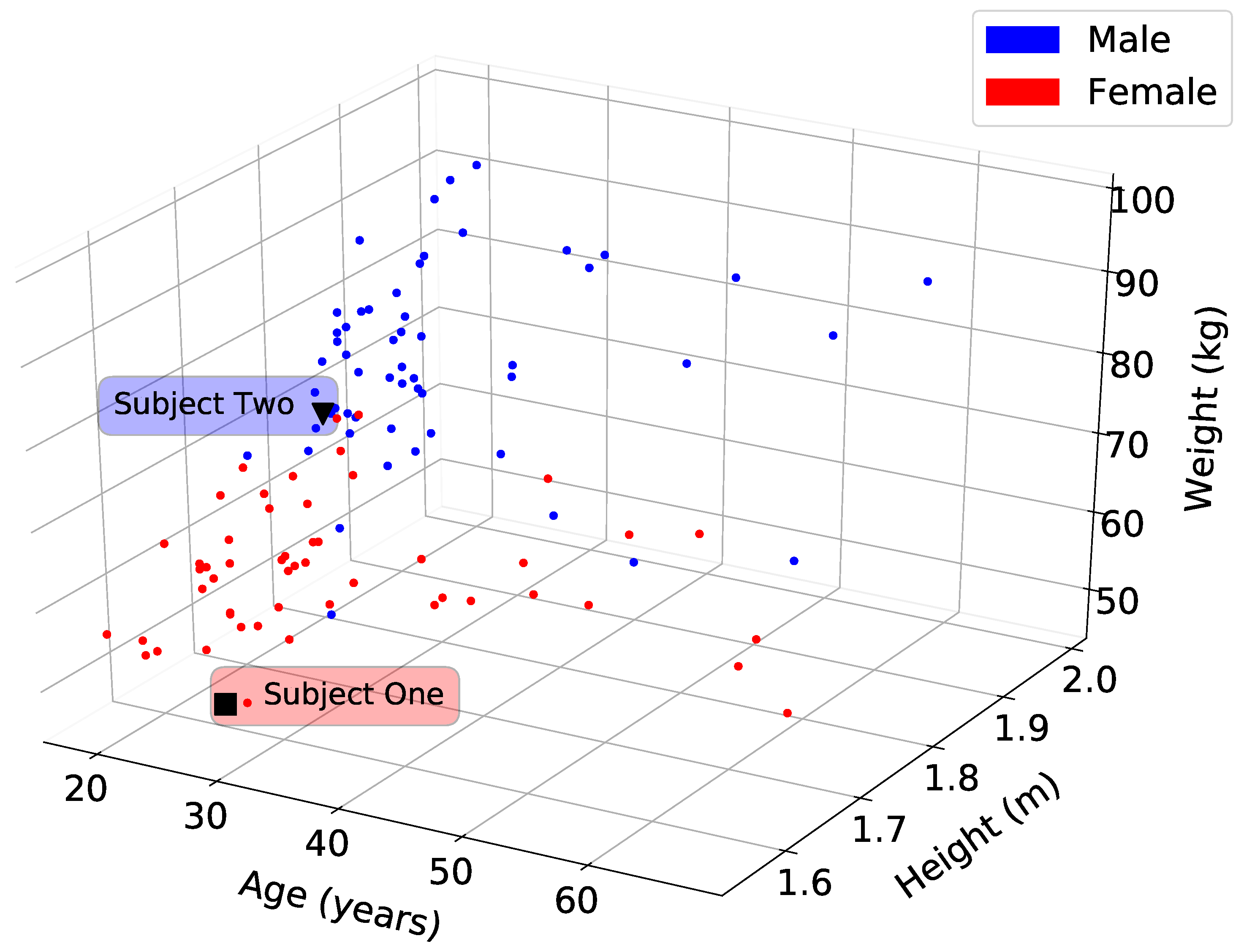
In this study, we considered one hundred and nine healthy adults who range in physical characteristics (e.g., height, weight, mass, age). We used two public databases that cumulatively provided 4079 full cycles of gait, and our own database, which provided 124 cycles of gait. Moissenet database [13] used 51 participants, Horst database [14] used 56 participants, and our database used 2 participants (See Table A9). In our experiments we used a set of in-house developed 9-degrees of freedom orientation IMU sensor with a 3-axis magnetometer, 3-axis gyroscope, and 3-axis accelerometer that used the Madwick sensor-fusion algorithm to calculate angular displacement and wirelessly transmit the information to a remote host using the TCP protocol [17,22]. Figure 1 shows the correlation between the age, height, and weight for all of the participants.
Since each database had its unique recording strategy (e.g., different marker placement and different sampling rate), the experimental data were preprocessed using Algorithm 1 to include marker numbers, frames, samples, mass, gender, and height into a single matrix representing each subject’s biometrics [23]. For example, the Moissenet and our own databases were sampled at 100 Hz, while the Horst database was recorded at 250 Hz. We downsampled Horst database to match the other two sets of data and generate a training data set that consists of over 700,000 samples at 100 Hz. It is important to note that the markers and their locations for both the Moissenet and Horst databases were interpreted by BioMechZoo solvers to output a joint angle relationship that yielded similar ranges of motion. Both of these databases included foot–ground reaction forces. We simulated the ground reaction force using “the simulated force plate” component available in OpenSim.
| Algorithm 1: Data Preparation Pipeline |
 |
The organization of the data structure for the recorded motion (T) shown in Equation (1), contains a Cartesian markers (), frame number (f), and individual trials or samples (i).
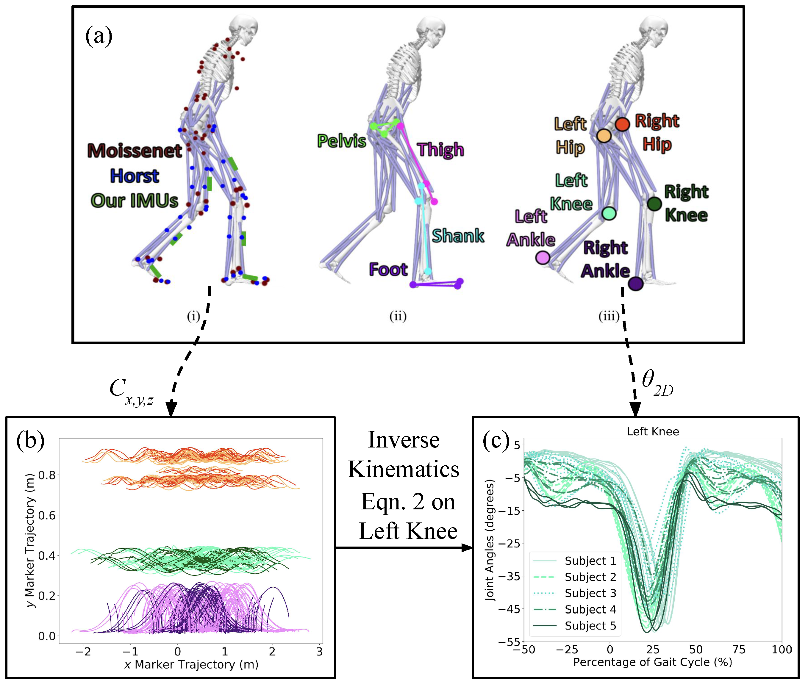
Figure 2 illustrates the process of extracting Cartesian coordinates from raw marker data and convert them into joint angles. This means that our system is capable accepting different sources of motion capture, and the pre-processing pipeline from Algorithm 1, we convert the data sets into a consistent parent–child joint angle relationship for all subjects. To clean up the data set, we scripted Equation (2) to determine the joint angle representation along the sagittal plane (Figure 3) for the lower extremity joints [13,14]. After the joint angles were found for all participants, we verified the alignment for all calculated joint angles to ensure they are in the same range of motion.
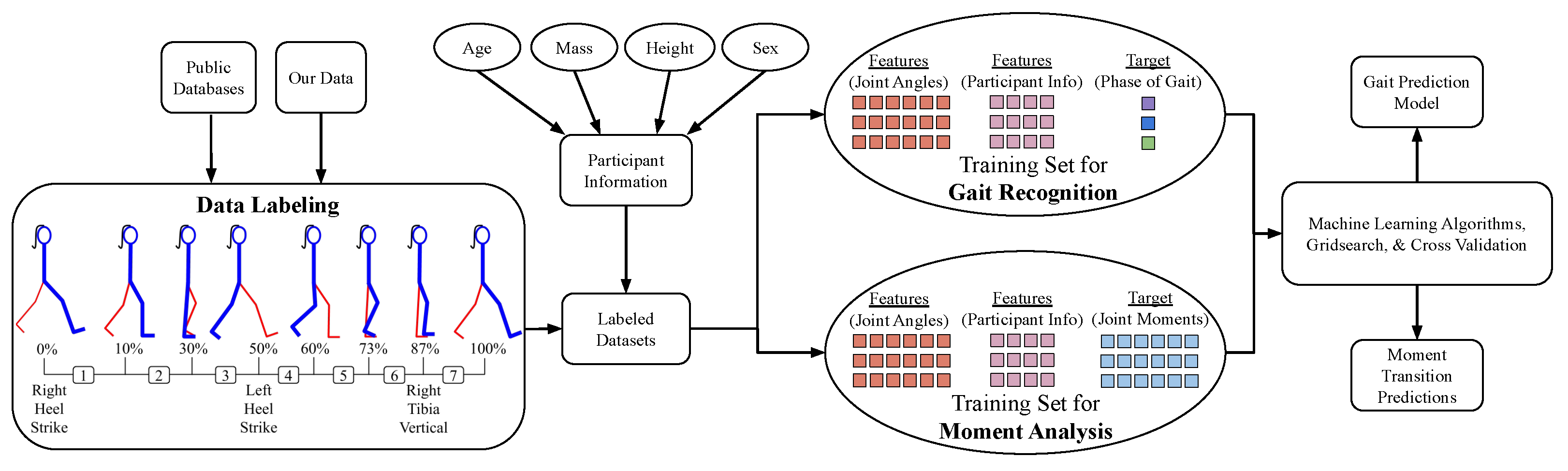
In some cases there exists multiple trials of the same subject, but in the event the participant changed, all of the subjects attributes (S): gender (g), mass (m), height (h), and age (a) were assigned as a new person. After the data sets have been labeled for phase of gait (P), subject attributes (S), and joint angle kinematics (), we transitioned into the process for training both the Gait Prediction and Moment Transition Predictions (Figure 4).
2.2. Classification Techniques and Algorithms
Machine learning automates the process of interpreting large sets of data to learn and make estimations [24] as well as construct a model to perform data-driven classifications. One of the primary goals of this work was to create a model that can accurately predict the phase of gait using joint angles. The model is trained to find a correlation between the input features (i.e., the observed and recorded input data) and the output targets (i.e., different phases of gait). This correlation is used to calculate targets for stand-alone or unlabeled features. The accuracy of each model is evaluated by interpreting how well the correlation can be found by the algorithm to predict the target using the features with cross validation.
In this work we used cross-validation to quantify the performance of each model. We split a certain percentage of the labeled data to use as test data, while the remaining data was used to train a model [25]. The training data is used as an input into the model, and the output was compared to its observed target to evaluate the accuracy against the other portion of the data set. Cross-validation iterates through the set of data multiple times, where each interval selects a different set of data samples to test, providing a more consistent performance metric of the entire model [25]. The calculations from cross validation were used as a metric for accuracy to compare with the outputs of each model we train.
We used the k-Nearest Neighbors (KNN) algorithm to classify the test features based on the most frequent phase of gait of their k surrounding neighbors, or closest data samples [26]. The parameter, k, defines how many neighbors were used in each classification. A relatively larger k results in a more accurate classification due to a larger scope of data. This reduces the effect of outliers and erroneous data for each prediction. The KNN algorithm has been used in other instances of training models for gait recognition based on different bio-mechanic features, including accelerometer data [27], ground reaction forces [28], and human gait shape analysis [29].
To find the nearest neighbors of each test sample, we calculated the Euclidean distance, D, between the feature sets of the test and already classified samples [30]. Each feature can be represented as:
with n representing the number of features in each sample, and every representing one feature. A feature vector for one sample combines all relevant features for training:
The distance D between the test feature set x and the already classified feature set y can be represented with the following formula:
where the iterator, i, increments for every feature used to train the model [30]. Equation (4) was evaluated for all training data samples, y. The number of samples (k) used in the training data set with the smallest distance (D) was selected as the test sample’s k nearest neighbors. The mode target value, or most frequent phase of gait within the selected neighbors, was used as the classification of the test sample x (Figure 5) [26]. This process was repeated to predict a phase of gait for each test feature set. Cross-validation repeats until all 10 folds and splits are iterated and completed. Generally, as k increases, the accuracy of the prediction increases as more data points are considered for the final classification. Decreasing k heightens the effect of inaccurate data on classifications; the balance for an ideal value of k is described using GridSearch. GridSearch finds specified parameter values through an exhaustive search process [31]. It sorts through all possible combinations of each parameter and finds the optimal values (Table A1). Both GridSearch and feature extraction optimize the parameters of our model and the features considered to heighten the efficiency of our model for training.
We used GridSearch to programmatically iterate through different combinations of parameter values (Table A1) to find the ideal values to run the model with [32]. When applied to the KNN algorithm, it varies the number of neighbors in each classification, k, to find a balance between the model over-fitting and under-fitting our data. If the number of neighbors was small, the effect of noise on the classification become larger since the model only learned from a small subset of neighbor samples. When outliers heavily influence the model, we notice a bias towards the minor details of the data (over-fitting) rather than finding a general trend [33]. However if k is large, we notice the opposite since every test sample will be classified to the target (under-fitting). This happens to be more frequent than a smaller k in the overall training set, ignoring underlying trends in the data [33]. Finding a balance of the value of k is crucial to achieve an accurate and precise model.
We used the Classification And Regression Trees (CART) algorithm to focus on creating a decision tree that classifies the test samples [34]. Decision trees are commonly used in many situations where supervised learning is practical: forming gait pattern models using other features such as inhibitory factors of an injury [35], contact forces and angular velocity [36], as well as step length, walking speed, and stride time [37].
Each tree consists of nodes, branches, and leaves. Nodes are known as a “decision”, or a comparison or split made on a specific feature in the data set. Branches are the outcome of the decision made by the node. A leaf is a node at the end of the tree that does not have branches extending from it. It is important to note that leaf nodes do not make decisions. Each leaf represents a target or a specific phase of gait. When making a classification, the data presented in our test feature set compares each node by traversing along the corresponding branches until it reaches a leaf node [34].
When training quantitative data, each node splits at a specific feature value. In our case, a node concerning right hip angles could split at . This creates the left branch at for the right hip node, and for the right branch. The ideal split yields both branches as a completely homogeneous pool of data points with the same target. Each branch splits into more nodes until every leaf node is either a product of a perfect split or until the tree reaches the maximum depth or width as specified by the parameters. The Gini impurity (I) is a quantitative measure of how accurate a split is. Ideal splits have a Gini impurity value of 0 [38], and is calculated as follows:
where t = 7 is the number of targets, and is the probability of selecting a data point with target i within the entire data set.
The feature with the smallest Gini impurity is chosen as the root of the tree. In other words, if we randomly classified according to the target distribution of the data set, the feature with the smallest possibility of incorrect classification is the root (see Figure 5) [39]. Once we select a feature as the root node and splits according to the smallest Gini impurity value, choosing the next node and split is repeated with the data subset of each branch until a complete tree has formed. As seen in Figure 5, our classification in a decision tree followed the splits made by the nodes for a test feature set until a leaf node, or target, is reached.
The parameters of maximum depth and width of a decision tree prevent the common problem of overfitting in decision trees [34]. Suppose we let the tree grow until every split reaches an impurity of 0. In that case, every feature set likely traces a unique path to an individual leaf node due to noise in the data, making the classification overfitted and heavily affected by every outlier. To prevent this, we restrict the number of splits and nodes through a tree’s maximum depth and width. GridSearch iterates through different threshold values, so the parameter values shown in Table A1 avoid underfitting and overfitting.
The random forest (RNDM) algorithm uses many different decision trees, as constructed in the CART algorithm, to create a forest [40]. The most frequent classification made among all the decision trees in the forest is the classification of test data points [40]. The logic behind using a forest of trees formed by randomly selected data samples and features is that the entire forest will have a low correlation between each tree. The product of uncorrelated models is far more accurate than any individual prediction. Similar to the wisdom of crowds, trees with erroneous data are protected by a more significant amount of trees with more accurate models.
We began the random forest algorithm developing each decision tree by creating a bootstrapped data set as portrayed in Figure 5 [40]. With repetition, a set of data samples randomly selected from the entire data set is the bootstrapped data set that will form our tree. Every bootstrapped data set has the same number of samples as the entire data set, so that most bootstrapped sets include the repetition of random samples.
For each bootstrapped data set, decision trees were formed with a random selection of m features. Typically , with n being the total number of features in the data set (Figure 4). The process of creating a decision tree (Algorithm 2) uses each tree formed from calculating Gini impurity to determine the order of features as nodes and the optimal split per node. The process of building different bootstrapped data sets and creating decision trees with random subsets of features for each bootstrapped group repeats until the maximum number of trees t is reached. When classifying a test sample with the random forest algorithm, a test feature set serves an an input into all the decision trees in the forest. The most frequent target output of the trees is the classification derived from the test data.
The random forest algorithm is optimized using the parameters m, the number of features used in each tree, and t, the number of trees in a forest (Table A1). A GridSearch through both these parameters usually reveals an increase in accuracy with the typically selected value of m = , and a larger t to account for more significant variation in datasets. GridSearch is essential to prevent underfitting and overfitting in the RNDM algorithm due to the randomness of sample and feature selection.
| Algorithm 2: Classification of phase of gait in relation to joint angles using Random Forest. |
 |
2.3. Extra Trees Regressors
Regression is another approach of supervised machine learning that outputs numerical values as a target, rather than as a category [41]. The previous KNN and decision tree algorithms are applied as regression techniques by changing the target from categories into continuous values. For example, a KNN classification can be turned into regression by averaging the numerical targets of the k nearest neighbors rather than taking the most categorical frequent target. Similarly, the leaves become prediction values rather than categories in a regression algorithm in algorithms with decision trees.
The extra trees algorithm is very similar to the random forest algorithm, creating many decision trees to form a forest. However, there are two critical differences between random forest and extra trees. Extra trees do not use a bootstrapped dataset like random forest. Each decision tree was formed by every sample in the entire training set [42]. Additionally, the extra trees algorithm uses a random split while creating decision trees, rather than calculating the optimal split with weighted Gini impurities like a typical decision tree [42]. Although, it is essential to note that extra trees still use Gini to calculate feature importance. Predictions in extra trees are made by averaging the output of all the trees in the forest for every test sample set [42]. When employing GridSearch in extra trees regression, the same parameters iterated through during the random forest algorithm are optimized (Table A1) so that the decision trees that make up the forest do not underfit or overfit the dataset.
2.4. Algorithm Applications
The classification algorithms (KNN, CART, Random forest) use the feature set that included joint angles (right and left hip, knee, and ankle) and participant information (e.g., height, mass, gender, age). Our feature set comprises 10 individual features, 6 joint angles, and 4 participant attributes. The target is the individual phase of gait for each data sample. We employ a 10-fold cross-validation and a 20/80 train–test split across all models when evaluating accuracy. The data is iterated 10 separate times during cross-validation to evaluate the accuracy. Each iteration selects a different 20% portion of the data set to reserve as sample test data points while the other 80% is selected as training data for the model.
Before selecting specific algorithms to use, we bench-marked the mean accuracy (with the standard deviation) in Table A5 using cross-validation on 10-fold experiments for a sample set employing all available features to help us narrow our chosen algorithms to KNN, CART, and RNDM. It is important to note that the parameters found from cross-validation and GridSearch mentioned in the previous sections were consistent for all feature combinations. The Naive Bayes (NB) and Support Vector Machine (SVM) algorithm produced models with relatively low accuracy compared to the other algorithms. As a linear classifier, the NB algorithm was unfit for our human gait classification with natural variances. The inefficiency of the SVM classifier with the Radial Basis Function (RBF) kernel and its proneness to over-fitting given larger data sets makes it unsuitable for training our model, and its shortcomings are prevalent in a 22% average decrease in accuracy compared to the algorithms we employed (Table A5). In addition, this SVM algorithm is particularly sensitive to noise, which makes it unsuitable for classifying our data with human variation. Therefore, we chose a final selection of the KNN, CART, and Random forest algorithms for our phase of gait prediction.
Since joint moments are only calculated for the subset of .mot data processed through OpenSim, we use regression techniques to roughly predict the moments corresponding to the joint angles from the .c3d files. In this scenario, the joint angles and participant information are the features, while we have a multi-class target: the moments for each of the six joints. By calculating moments for every test sample, we observed the trends of joint moments over each phase to approximate the maximum moment needed to move from one phase to the next, an addition to our overall gait pattern model.
To predict joint moments from the joint angles extracted from .c3d files, we created a model with the extra trees regressor using joint angles and moments from OpenSim. Our features were joint angles and participant information, and our targets were joint moments. A separate model was created for each phase, as seen in Figure 6. The regression accuracy calculated by cross-validation for each model is recorded in Table A7, where each model’s coefficient of determination exceeds 0.5, meaning each model accounts for a majority of the variance of the outputted moments. For this application, where joint angle trends varied greatly with each participant and even between each gait cycle, the extra trees outperformed all other regression algorithms due to the randomness in splitting nodes to smooth noise in the data set. It is important to note that due to the variance of subjects’ physical characteristics (i.e., subjects can be very small to large), the regression accuracy per phase may seem lower than normal. This does not affect the system’s ability to take physical characteristics and derive a estimation on required moments to transition between phases of gait.
3. Results and Discussion
The typical application for monitoring human gait focuses on the stance–swing transitions for cycle tracking (95% accuracy) [43], or rely heavily on the measurements on the foot (98% accuracy) [44]. This work aims to be less biased and dependent on a specific body part (in the event there is limb loss), and instead demonstrates the numerical trade-offs between tracking different joints on the human body. To increase the efficiency of our model, we reduced the number of features used while training to reduce the training run-time and ease the process of data collection [19]. Our models used a maximum of n = 10 features to train: joint angles ( = 6), and four participant attributes. Each test included the four participant attributes while training a model,
where the joint angle feature combinations are iterated through to find the ideal combination of the least number of features n and highest accuracy. This method trained the models ranging from just one joint angle, or all six, meaning the model trains on a minimum of five features and a maximum of ten. Some joints reveal themselves to affect the correlation between features and target more than others after analyzing the accuracy of the model of each joint combination.
As previously mentioned, the feature set, or input into the model, compromises of six joint angles and four participant attributes. The target, and eventual output of the models, is the individual phase of gait for each data sample. We used a 10-fold cross-validation and a 20/80 train–test split across all models when evaluating accuracy in recognizing the collection of joint angles. The data is iterated during cross-validation to evaluate the accuracy between the labelled data set as well as for parametric configurations. To find the performance of our models against the labeled data versus predicted data, we used confusion matrices to find mean accuracy (Table A2, Table A3 and Table A4). If the model yields the correct phase of gait given the joint angle(s) compared with the labeled data set, that is considered a successful prediction. Hip joint angles are particularly effective in training the model (Figure 7), and models training with KNN using feature combinations with just three joint angles can reach over 85% accuracy with one or both hip joint features. The CART algorithm also undergoes the same feature selection process among 63 feature combinations and achieves over 84% accuracy with just three joint angle features, slightly underperforming the KNN algorithm. The RNDM algorithm involved the same overall feature selection in the data set as other algorithms with 63 feature combinations. Random forest outperforms both KNN and CART (Figure 7) and was able to reach over 87% accuracy with just three features, revealing the importance of randomness when analyzing human data. Refer to Figure 7, which shows a significant association between both the hip joint angles and higher accuracy for all algorithms and combinations of joint angles.
Due to the nature of unique gait motions across individuals, we focused on the strong connection between phase of gait, joint angles, and joints’ moments. Focusing on the lower extremity joint angles for human gait is informative enough for phase classification. This approach can bridge this form of kinematic analysis toward joint dynamics. It is a well-known challenge to generalize the required moments from phase to phase for all subjects, but by taking advantage of OpenSim’s inverse dynamics solver (ID):
We purposed our joint angles for generalizing moments:
where represented the generalized forces, m is the mass, is angular velocity, is angular acceleration, G is gravitational forces, and is the joint angles from Equation (2). Our Moment Prediction Model (Figure 6) interpreted those joint angles () and predicted the maximum moments (Nm/kg) to transition between phases of gait. This correlation between joint angles, moments, and phase of gait aim to deliver an extremely adaptable model. The output (Figure 8) has the potential to be applied as a bookmark or characterization for assistive technologies to replicate given the physical characteristics of their users.
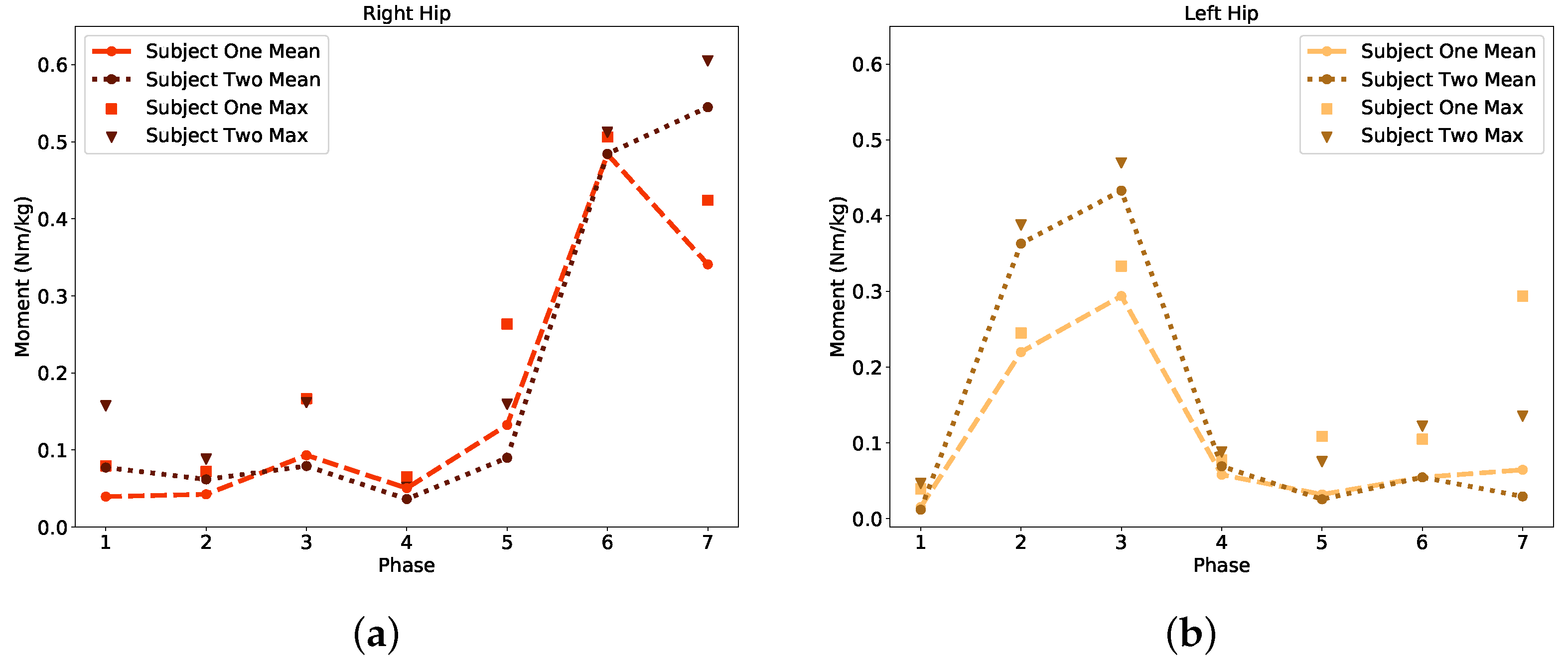
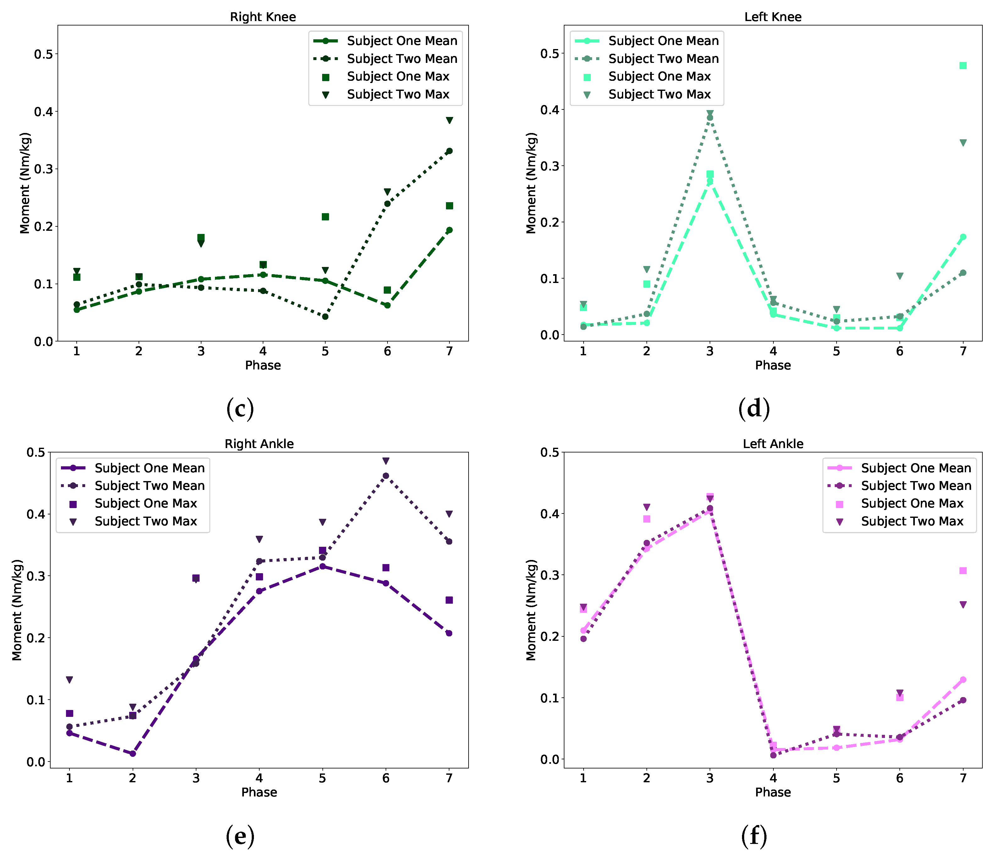
Typically healthy humans follow a very similar gait pattern. However, it is important to note that there are still noticeable differences between Subject One’s and Subject Two’s phase of gait and joint moment relationship (e.g., Phase 6 in Figure 8c). The results demonstrate that each person’s gait is unique in relying on different joints to move. Subject One is a 28-year-old female that is 1.56 m in height, and weighs 50 kg. Subject Two, a 23-year-old male that is 1.76 m tall and weighs 73 kg, shows more of a minor moment requirement to transition between phases of gait than Subject One. It is essential to recognize that both subjects were chosen from different databases, yet they yielded similar trends. For example, monitoring the left knee in Figure 8d indicated that Subject Two had a larger moment to transition from Phase 3 to 4 with a 31% difference compared to Subject One (Table A8). Yet, they followed similar moment requirements in a scaled proportion.
The observation in Figure 8 showed that Subject One had a stronger dependency on the left side of the body, and Subject Two was more evenly distributed with a slight bias to the right side of the body. The assessment from both the gait classification and moment prediction models demonstrated a fundamental breakdown in the analysis of walking movement and can be further implemented as a valuable tool for biometric technologies.
4. Conclusions
This paper proposes a machine learning method to identify the phase of gait from joint angle measurements and generalize a set of required joint moments between those phases of gait along the sagittal plane. We used the algorithms KNN, CART, and RNDM to yield an 82%, 87%, and 92% accuracy in gait phase classification with all available features or lower extremity joints. Our understanding of how feature reduction affected the confidence of our RNDM classification model (Table A6) indicated how reliable monitoring fewer joint angles could be. Figure 7 proved this analysis by showing how the amount of joints required for monitoring each subject affects the accuracy of gait phase prediction. It is clear that the more sensors or features monitored, the higher the confidence; however, the difference between tracking six joints to five joints (0.5%), or six joints to three joints (4.04%) has a very minimal drop-off in accuracy. This finding indicates that reducing the number of joints monitored for complex gait phase-reliant applications will yield promising results. It is important to note that flexibility of joints is entirely individualized, where age or gender might demonstrate their own significant variance. For this work, we focused on the relationship between the physical characteristics and angular displacement of joints for human subjects. The authors believe future applications of this work could include: biomechanic comparisons between age and gender [45], robotic assistive devices, and motion not confined to the sagittal plane.
We correlated the exact joint angle measurements and phases of gait to yield each subject’s moments. Figure 8 and Table A8 demonstrate how a smaller Subject One requires smaller moments to transition between phases of gait than a physically larger Subject Two. Generally, both subjects in Figure 8 follow similar trends, but differences like Phase 6 for the Right knee show a considerable uniqueness between persons. The difference between results demonstrated how body size affected the required maximum moments proportionally. Correlating the joint angle relationships between the two modes for gait prediction and moment transitions (Figure 4) can be used as a powerful tool for biometric applications. Using the same database for two different applications bridges the IK and ID area of biomechanic analysis proving the impact of joint angle measurement techniques. Implementing IMU sensors for biometric analysis reduces the cost, room-bounded configurations, and overall complexity of optical motion capture systems.
Author Contributions
Conceptualization, E.J., C.L. and M.C.; methodology, E.J., C.L.; software, C.L. and E.J.; validation, E.J., C.L. and M.T.; formal analysis, E.J. and C.L.; investigation, C.L. and E.J.; resources, E.J., C.L. and M.C.; data curation, C.L. and E.J.; writing—original draft preparation, C.L., E.J.; writing—review and editing, E.J., C.L., M.C. and M.T.; visualization, C.L. and E.J.; supervision, E.J.; project administration, M.T.; funding acquisition, M.T. All authors have read and agreed to the published version of the manuscript.
Funding
This research was supported by a grant made to the Braingeneers research group by Schmidt Family Futures. The funders had no role in study design, data collection and analysis, decision to publish, or preparation of the manuscript.
Institutional Review Board Statement
Under an UCSC IRB Protocol #HS3588, we have been able to collect motion captured data of a person.
Informed Consent Statement
We collected data on ourselves within this study, and the subject signed written informed consent as part of the UCSC IRB Protocol.
Data Availability Statement
Public archived datasets used in this study include Moissenet et al.: https://figshare.com/articles/A_multimodal_dataset_of_human_gait_at_different_walking_speeds/7734767 (accessed on 13 December 2021), and Horst et al.: https://data.mendeley.com/datasets/svx74xcrjr/3 (accessed on 13 December 2021). Additional data availability will be given upon request to the corresponding author.
Conflicts of Interest
The funders had no role in the design of the study; in the collection, analyses, or interpretation of data; in the writing of the manuscript, or in the decision to publish the results.
Abbreviations
| inverse of the mass matrix | |
| angular acceleration | |
| vector for accelerations | |
| vector for velocities | |
| angular velocity | |
| vector of generalized forces | |
| joint angles along sagittal plane | |
| individual trials or samples | |
| frame number | |
| marker number | |
| vector of Coriolis and centrifugal forces | |
| Cartesian markers | |
| feature set | |
| feature vector | |
| q | vector of generalized positions |
| R | random set of samples |
| generalized forces | |
| a | age |
| CART | Classification And Regression Trees algorithm |
| D | distance between feature sets |
| F | forces |
| G | gravitational forces |
| g | gender |
| h | height |
| I | Gini impurity |
| KNN | K-Nearest Neighbors algorithm |
| L | labeled data set |
| M | moments |
| m | mass |
| N | number of features when branching |
| n | total number of features |
| P | phase of gait |
| r | force plate responses |
| RNDM | Random forest algorithm |
| S | subject data |
| T | motion captured database |
| t | number of trees |
Appendix A

Table A1.
Using GridSearchCV with the scikit learn tools, the best parameters were found for KNN, CART, and RNDM, where each algorithm went through a 10 fold and split using cross-validation.
Table A1.
Using GridSearchCV with the scikit learn tools, the best parameters were found for KNN, CART, and RNDM, where each algorithm went through a 10 fold and split using cross-validation.
| KNN | CART | RNDM | |||
|---|---|---|---|---|---|
| algorithm | auto | ccp alpha | 0.0 | bootstrap | True |
| leaf size | 30 | class weight | None | ccp alpha | 0.0 |
| metric | minkowski | criterion | gini | class weight | None |
| metric params | None | max depth | None | criterion | gini |
| n jobs | None | max features | None | max depth | None |
| n neighbors | 10 | max leaf nodes | None | max features | sqrt |
| p | 2 | min impurity decrease | 0.0 | max leaf nodes | None |
| weights | distance | min impurity split | 1 | max samples | None |
| min samples split | 5 | min impurity decrease | 0.0 | ||
| min weight fraction leaf | 0.0 | min impurity split | None | ||
| presort | deprecated | min samples leaf | 1 | ||
| random state | None | min samples split | 5 | ||
| splitter | best | min weight fraction leaf | 0.0 | ||
| n estimators | 250 | ||||
| n jobs | None | ||||
| oob score | False | ||||
| random state | None | ||||
| verbose | 0 | ||||
| warm start | False |
Table A2.
K-Nearest Neighbors Classification report with a confusion matrix for all the phases of gait (left) and scores (right).
Table A2.
K-Nearest Neighbors Classification report with a confusion matrix for all the phases of gait (left) and scores (right).
| 1 | 2 | 3 | 4 | 5 | 6 | 7 | Precision | Recall | F1-Score | Support | ||
|---|---|---|---|---|---|---|---|---|---|---|---|---|
| 1 | 18,885 | 1140 | 19 | 7 | 54 | 18 | 1149 | 7 | 0.89 | 0.89 | 0.89 | 21,272 |
| 2 | 1145 | 17,179 | 864 | 10 | 33 | 47 | 8 | 6 | 0.89 | 0.89 | 0.89 | 19,286 |
| 3 | 25 | 928 | 14,827 | 807 | 28 | 100 | 37 | 5 | 0.89 | 0.89 | 0.89 | 16,746 |
| 4 | 13 | 7 | 814 | 10,169 | 778 | 37 | 51 | 4 | 0.86 | 0.86 | 0.86 | 11,869 |
| 5 | 29 | 28 | 20 | 765 | 22,132 | 824 | 32 | 3 | 0.92 | 0.93 | 0.93 | 23,830 |
| 6 | 9 | 27 | 55 | 18 | 889 | 28,913 | 1183 | 2 | 0.93 | 0.93 | 0.93 | 31,094 |
| 7 | 1194 | 5 | 20 | 28 | 26 | 1200 | 14,700 | 1 | 0.86 | 0.86 | 0.86 | 17,173 |
| accuracy | 0.90 | 141,270 | ||||||||||
| macro avg | 0.89 | 0.89 | 0.89 | 141,270 | ||||||||
| weighted avg | 0.90 | 0.90 | 0.90 | 141,270 |
Table A3.
Classification and Regression Trees Classification report with a confusion matrix for all the phases of gait (left) and scores (right).
Table A3.
Classification and Regression Trees Classification report with a confusion matrix for all the phases of gait (left) and scores (right).
| 1 | 2 | 3 | 4 | 5 | 6 | 7 | Precision | Recall | F1-Score | Support | ||
|---|---|---|---|---|---|---|---|---|---|---|---|---|
| 1 | 17,894 | 1404 | 51 | 22 | 67 | 27 | 1807 | 7 | 0.84 | 0.84 | 0.84 | 21,272 |
| 2 | 1321 | 16,452 | 1366 | 25 | 49 | 55 | 18 | 6 | 0.85 | 0.85 | 0.85 | 19286 |
| 3 | 38 | 1411 | 14,037 | 1041 | 57 | 118 | 44 | 5 | 0.84 | 0.84 | 0.84 | 16,746 |
| 4 | 26 | 23 | 1099 | 9334 | 1264 | 61 | 62 | 4 | 0.79 | 0.79 | 0.79 | 11,869 |
| 5 | 50 | 35 | 72 | 1229 | 21,234 | 1171 | 39 | 3 | 0.89 | 0.89 | 0.89 | 23,830 |
| 6 | 32 | 64 | 94 | 64 | 1267 | 27,874 | 1699 | 2 | 0.90 | 0.90 | 0.90 | 31,094 |
| 7 | 1847 | 13 | 54 | 70 | 43 | 1735 | 13,411 | 1 | 0.79 | 0.78 | 0.78 | 17,173 |
| accuracy | 0.85 | 141,270 | ||||||||||
| macro avg | 0.84 | 0.84 | 0.84 | 141,270 | ||||||||
| weighted avg | 0.85 | 0.85 | 0.85 | 141,270 |
Table A4.
Random Forest Classification report with a confusion matrix for all the phases of gait (left) and scores (right).
Table A4.
Random Forest Classification report with a confusion matrix for all the phases of gait (left) and scores (right).
| 1 | 2 | 3 | 4 | 5 | 6 | 7 | Precision | Recall | F1-Score | Support | ||
|---|---|---|---|---|---|---|---|---|---|---|---|---|
| 1 | 19,106 | 855 | 18 | 8 | 46 | 10 | 1229 | 7 | 0.89 | 0.90 | 0.90 | 21,272 |
| 2 | 974 | 17,381 | 850 | 4 | 31 | 40 | 6 | 6 | 0.90 | 0.90 | 0.90 | 19,286 |
| 3 | 33 | 990 | 14,833 | 737 | 24 | 98 | 31 | 5 | 0.89 | 0.89 | 0.89 | 16,746 |
| 4 | 13 | 9 | 823 | 10,118 | 839 | 31 | 36 | 4 | 0.87 | 0.85 | 0.86 | 11,869 |
| 5 | 32 | 22 | 22 | 785 | 22,207 | 741 | 21 | 3 | 0.92 | 0.93 | 0.93 | 23,830 |
| 6 | 15 | 28 | 39 | 16 | 881 | 29,053 | 1062 | 2 | 0.93 | 0.93 | 0.93 | 31,094 |
| 7 | 1228 | 5 | 19 | 26 | 22 | 1304 | 14,569 | 1 | 0.86 | 0.85 | 0.85 | 17,173 |
| accuracy | 0.90 | 141,270 | ||||||||||
| macro avg | 0.89 | 0.89 | 0.89 | 141,270 | ||||||||
| weighted avg | 0.90 | 0.90 | 0.90 | 141,270 |
Table A5.
Accuracy of prediction (%) of Cross-Validation (CV) on 10-fold experiments using Linear, CART, KNN, and RNDM using all available features.
Table A5.
Accuracy of prediction (%) of Cross-Validation (CV) on 10-fold experiments using Linear, CART, KNN, and RNDM using all available features.
| Classifier | KNN | CART | NB | SVM | RNDM |
|---|---|---|---|---|---|
| Mean (± SD) | 0.902 (± 0.012) | 0.857 (± 0.018) | 0.796 (± 0.017) | 0.665 (± 0.023) | 0.905 (± 0.011) |
Table A6.
Using feature reduction, we can demonstrate the correlation between number of joints (features) and mean accuracy (%) using Random Forest classifier. It is worth noting that 6 has only 1 combination of features, but the rest follow the format: max accuracy % (mean %).
Table A6.
Using feature reduction, we can demonstrate the correlation between number of joints (features) and mean accuracy (%) using Random Forest classifier. It is worth noting that 6 has only 1 combination of features, but the rest follow the format: max accuracy % (mean %).
| Number of Features | 6 | 5 | 4 | 3 | 2 | 1 |
|---|---|---|---|---|---|---|
| KNN | 90.8 | 90.6 (90.1) | 89.3 (88.7) | 86.7 (85.4) | 79.7 (75.0) | 49.6 (47.3) |
| CART | 87.9 | 87.1 (87.0) | 86.2 (85.6) | 84.1 (82.4) | 76.4 (71.0) | 45.8 (43.1) |
| RNDM | 91.7 | 91.2 (91.1) | 90.0 (89.8) | 87.6 (86.6) | 79.8 (75.3) | 45.8 (43.2) |
Table A7.
A table of the regression accuracy per phase when generating the Extra Trees model to predict joint moments from joint angles. The accuracy is the coefficient of determination, , of the prediction. The best possible score is 1.0.
Table A7.
A table of the regression accuracy per phase when generating the Extra Trees model to predict joint moments from joint angles. The accuracy is the coefficient of determination, , of the prediction. The best possible score is 1.0.
| Phase of Gait | Regression Accuracy ( Error) |
|---|---|
| 1 | 0.567 |
| 2 | 0.592 |
| 3 | 0.713 |
| 4 | 0.840 |
| 5 | 0.568 |
| 6 | 0.727 |
| 7 | 0.505 |
Table A8.
Required moment transitions between gait cycles as predicted by Random Forest regression for Subject One, Subject Two, and All Partipicants. See Figure 1 for physical characteristics (e.g., mass, height, weight).
Table A8.
Required moment transitions between gait cycles as predicted by Random Forest regression for Subject One, Subject Two, and All Partipicants. See Figure 1 for physical characteristics (e.g., mass, height, weight).
| Subject One | Moment (Nm/kg) | |||||
|---|---|---|---|---|---|---|
| Gait Transition | Right Hip | Left Hip | Right Knee | Left Knee | Right Ankle | Left Ankle |
| 0.080 (± 0.014) | 0.040 (± 0.011) | 0.110 (± 0.013) | 0.048 (± 0.015) | 0.777 (± 0.013) | 0.244 (± 0.021) | |
| 0.072 (± 0.018) | 0.245 (± 0.025) | 0.112 (± 0.020) | 0.090 (± 0.018) | 0.075 (± 0.013) | 0.391 (± 0.021) | |
| 0.167 (± 0.036) | 0.333 (± 0.033) | 0.180 (± 0.029) | 0.285 (± 0.030) | 0.297 (± 0.017) | 0.427 (± 0.029) | |
| 0.065 (± 0.010) | 0.078 (± 0.015) | 0.134 (± 0.024) | 0.042 (± 0.006) | 0.299 (± 0.011) | 0.022 (± 0.005) | |
| 0.263 (± 0.032) | 0.109 (± 0.021) | 0.216 (± 0.054) | 0.030 (± 0.004) | 0.341 (± 0.016) | 0.049 (± 0.015) | |
| 0.506 (± 0.002) | 0.105 (± 0.004) | 0.089 (± 0.006) | 0.030 (± 0.006) | 0.313 (± 0.008) | 0.100 (± 0.004) | |
| 0.424 (± 0.086) | 0.294 (± 0.074) | 0.236 (± 0.060) | 0.478 (± 0.118) | 0.261 (± 0.074) | 0.307 (± 0.060) | |
| Subject Two | Moment (Nm/kg) | |||||
| Gait Transition | Right Hip | Left Hip | Right Knee | Left Knee | Right Ankle | Left Ankle |
| 0.157 (± 0.002) | 0.047 (± 0.010) | 0.121 (± 0.015) | 0.054 (± 0.011) | 0.132 (± 0.020) | 0.247 (± 0.018) | |
| 0.088 (± 0.019) | 0.388 (± 0.020) | 0.122 (± 0.018) | 0.116 (± 0.016) | 0.088 (± 0.020) | 0.410 (± 0.0160) | |
| 0.162 (± 0.022) | 0.470 (± 0.033) | 0.169 (± 0.020) | 0.393 (± 0.013) | 0.294 (± 0.009) | 0.424 (± 0.010) | |
| 0.051 (± 0.008) | 0.088 (± 0.010) | 0.132 (± 0.020) | 0.062 (± 0.004) | 0.359 (± 0.015) | 0.013 (± 0.0027) | |
| 0.159 (± 0.009) | 0.075 (± 0.015) | 0.123 (± 0.011) | 0.045 (± 0.007) | 0.387 (± 0.017) | 0.048 (± 0.004) | |
| 0.512 (± 0.004) | 0.122 (± 0.006) | 0.260 (± 0.002) | 0.104 (± 0.005) | 0.485 (± 0.009) | 0.107 (± 0.007) | |
| 0.605 (± 0.038) | 0.135 (± 0.017) | 0.384 (± 0.017) | 0.341 (± 0.033) | 0.340 (± 0.025) | 0.251 (± 0.022) | |
| All Participants | Moment (Nm/kg) | |||||
| Gait Transition | Right Hip | Left Hip | Right Knee | Left Knee | Right Ankle | Left Ankle |
| 0.109 (± 0.062) | 0.102 (± 0.072) | 0.127 (± 0.039) | 0.118 (± 0.080) | 0.109 (± 0.062) | 0.295 (± 0.097) | |
| 0.104 (± 0.065) | 0.270 (± 0.117) | 0.122 (± 0.063) | 0.116 (± 0.050) | 0.104 (± 0.064) | 0.387 (± 0.052) | |
| 0.130 (± 0.030) | 0.435 (± 0.239) | 0.189 (± 0.056) | 0.331 (± 0.130) | 0.131 (± 0.031) | 0.354 (± 0.152) | |
| 0.083 (± 0.028) | 0.111 (± 0.063) | 0.146 (± 0.021) | 0.080 (± 0.036) | 0.086 (± 0.041) | 0.055 (± 0.039) | |
| 0.194 (± 0.104) | 0.116 (± 0.096) | 0.181 (± 0.057) | 0.056 (± 0.042) | 0.197 (± 0.107) | 0.053 (± 0.025) | |
| 0.425 (± 0.232) | 0.089 (± 0.035) | 0.212 (± 0.124) | 0.066 (± 0.045) | 0.426 (± 0.231) | 0.064 (± 0.035) | |
| 0.0.439 (± 0.207) | 0.161 (± 0.128) | 0.264 (± 0.099) | 0.283 (± 0.177) | 0.438 (± 0.206) | 0.254 (± 0.138) | |
Table A9.
Participant Information used in Figure 1.
Table A9.
Participant Information used in Figure 1.
| Height | Age | Weight | |
|---|---|---|---|
| Male | 1.66 | 31 | 67 |
| Female | 1.64 | 48 | 65.4 |
| Female | 1.56 | 28 | 50 |
| Male | 1.77 | 23 | 72.5 |
| Male | 1.83 | 25 | 73.5 |
| Male | 1.76 | 23 | 73 |
| Female | 1.69 | 44 | 65 |
| Female | 1.66 | 30 | 57.1 |
| Male | 1.88 | 57 | 86 |
| Male | 1.8 | 59 | 63.4 |
| Female | 1.7 | 26 | 61.3 |
| Male | 1.8 | 29 | 92 |
| Female | 1.58 | 22 | 67 |
| Female | 1.76 | 26 | 73.8 |
| Female | 1.71 | 48 | 59.8 |
| Male | 1.92 | 33 | 87.5 |
| Female | 1.66 | 31 | 80.5 |
| Male | 1.89 | 38 | 89.9 |
| Female | 1.7 | 62 | 60.7 |
| Male | 1.77 | 21 | 67.2 |
| Female | 1.6 | 24 | 63.5 |
| Male | 1.84 | 21 | 89.6 |
| Female | 1.55 | 19 | 56.5 |
| Female | 1.65 | 40 | 61.8 |
| Female | 1.64 | 40 | 61.5 |
| Male | 1.74 | 32 | 72.2 |
| Female | 1.64 | 28 | 61.9 |
| Male | 1.91 | 25 | 88 |
| Male | 1.82 | 25 | 79.5 |
| Female | 1.72 | 21 | 62.8 |
| Male | 1.74 | 39 | 74 |
| Male | 1.77 | 52 | 87.2 |
| Female | 1.7 | 35 | 62 |
| Male | 1.9 | 48 | 89.4 |
| Female | 1.66 | 63 | 60.2 |
| Female | 1.69 | 58 | 73 |
| Female | 1.73 | 50 | 68 |
| Female | 1.69 | 46 | 76 |
| Female | 1.67 | 41 | 60.5 |
| Male | 1.79 | 43 | 95 |
| Female | 1.69 | 30 | 58 |
| Female | 1.71 | 64 | 51.5 |
| Male | 1.72 | 51 | 65.5 |
| Male | 1.87 | 24 | 86 |
| Male | 1.72 | 26 | 50.8 |
| Male | 1.77 | 38 | 81.5 |
| Male | 1.76 | 42 | 66.1 |
| Male | 1.88 | 31 | 74.8 |
| Male | 1.83 | 67 | 98 |
| Male | 1.78 | 21 | 74 |
| Male | 1.75 | 29 | 68.9 |
| Female | 1.81 | 21 | 64.9 |
| Male | 1.84 | 21 | 80.8 |
| Male | 1.82 | 23 | 82.7 |
| Female | 1.63 | 26 | 54.9 |
| Male | 1.79 | 21 | 77.3 |
| Male | 1.91 | 24 | 94.2 |
| Male | 1.88 | 23 | 69.5 |
| Male | 1.84 | 26 | 72 |
| Female | 1.58 | 20 | 52.3 |
| Female | 1.68 | 25 | 60.4 |
| Female | 1.64 | 23 | 55 |
| Female | 1.69 | 21 | 69.7 |
| Female | 1.69 | 26 | 59.3 |
| Female | 1.67 | 25 | 54.5 |
| Female | 1.75 | 23 | 57.4 |
| Female | 1.6 | 27 | 47.3 |
| Female | 1.62 | 22 | 61.4 |
| Male | 1.81 | 21 | 82.3 |
| Female | 1.69 | 19 | 65.6 |
| Female | 1.55 | 22 | 56.7 |
| Female | 1.61 | 26 | 56 |
| Male | 1.82 | 21 | 69.1 |
| Female | 1.62 | 22 | 62.1 |
| Male | 1.74 | 30 | 80.7 |
| Male | 1.99 | 21 | 91.2 |
| Male | 1.78 | 21 | 69.5 |
| Male | 1.83 | 24 | 67.5 |
| Female | 1.81 | 22 | 62.1 |
| Male | 1.81 | 28 | 81.35 |
| Female | 1.65 | 21 | 58.1 |
| Male | 1.78 | 23 | 80.9 |
| Female | 1.68 | 27 | 67.6 |
| Male | 1.78 | 23 | 82 |
| Female | 1.67 | 21 | 58.8 |
| Female | 1.69 | 24 | 59 |
| Female | 1.72 | 23 | 56.1 |
| Female | 1.61 | 23 | 52.1 |
| Male | 1.79 | 30 | 71 |
| Female | 1.58 | 21 | 53.15 |
| Female | 1.75 | 21 | 65.15 |
| Male | 1.83 | 25 | 79.95 |
| Female | 1.64 | 23 | 54.8 |
| Male | 1.82 | 21 | 76.5 |
| Male | 1.82 | 22 | 74.6 |
| Female | 1.65 | 20 | 56.45 |
| Male | 1.88 | 22 | 78.3 |
| Male | 1.92 | 22 | 90.8 |
| Male | 1.86 | 24 | 72.2 |
| Male | 1.87 | 22 | 81.8 |
| Female | 1.67 | 21 | 61.8 |
| Female | 1.61 | 30 | 55.75 |
| Male | 1.71 | 20 | 69.75 |
| Female | 1.7 | 22 | 66.15 |
| Male | 1.86 | 23 | 73.35 |
| Male | 1.79 | 22 | 71.75 |
| Male | 1.85 | 19 | 77.75 |
| Male | 1.778 | 24 | 69.85 |
| Male | 1.83 | 21 | 68.04 |
References
- Horst, F.; Lapuschkin, S.; Samek, W.; Müller, K.R.; Schöllhorn, W.I. Explaining the unique nature of individual gait patterns with deep learning. Sci. Rep. 2019, 9, 2391. [Google Scholar] [CrossRef] [PubMed] [Green Version]
- Prakash, C.; Kumar, R.; Mittal, N. Recent developments in human gait research: Parameters, approaches, applications, machine learning techniques, datasets and challenges. Artif. Intell. Rev. 2018, 49, 1–40. [Google Scholar] [CrossRef]
- Nashner, L. Adapting reflexes controlling the human posture. Exp. Brain Res. 1976, 26, 59–72. [Google Scholar] [CrossRef]
- Richards, R.E.; Andersen, M.S.; Harlaar, J.; Van Den Noort, J. Relationship between knee joint contact forces and external knee joint moments in patients with medial knee osteoarthritis: Effects of gait modifications. Osteoarthr. Cartil. 2018, 26, 1203–1214. [Google Scholar] [CrossRef] [Green Version]
- Seth, A.; Sherman, M.; Reinbolt, J.A.; Delp, S.L. OpenSim: A musculoskeletal modeling and simulation framework for in silico investigations and exchange. Procedia Iutam 2011, 2, 212–232. [Google Scholar] [CrossRef]
- Dixon, P.C.; Loh, J.J.; Michaud-Paquette, Y.; Pearsall, D.J. biomechZoo: An open-source toolbox for the processing, analysis, and visualization of biomechanical movement data. Comput. Methods Programs Biomed. 2017, 140, 1–10. [Google Scholar] [CrossRef]
- Pappas, I.P.; Popovic, M.R.; Keller, T.; Dietz, V.; Morari, M. A reliable gait phase detection system. IEEE Trans. Neural Syst. Rehabil. Eng. 2001, 9, 113–125. [Google Scholar] [CrossRef]
- O’Connor, C.M.; Thorpe, S.K.; O’Malley, M.J.; Vaughan, C.L. Automatic detection of gait events using kinematic data. Gait Posture 2007, 25, 469–474. [Google Scholar] [CrossRef]
- Jung, J.Y.; Heo, W.; Yang, H.; Park, H. A neural network-based gait phase classification method using sensors equipped on lower limb exoskeleton robots. Sensors 2015, 15, 27738–27759. [Google Scholar] [CrossRef]
- Farah, J.D.; Baddour, N.; Lemaire, E.D. Gait phase detection from thigh kinematics using machine learning techniques. In Proceedings of the 2017 IEEE International Symposium on Medical Measurements and Applications (MeMeA), Rochester, MN, USA, 7–10 May 2017; pp. 263–268. [Google Scholar]
- Begg, R.; Kamruzzaman, J. A machine learning approach for automated recognition of movement patterns using basic, kinetic and kinematic gait data. J. Biomech. 2005, 38, 401–408. [Google Scholar] [CrossRef]
- Zhou, H.; Hu, H. Human motion tracking for rehabilitation—A survey. Biomed. Signal Process. Control. 2008, 3, 1–18. [Google Scholar] [CrossRef]
- Schreiber, C.; Moissenet, F. A multimodal dataset of human gait at different walking speeds established on injury-free adult participants. Sci. Data 2019, 6, 1–7. [Google Scholar] [CrossRef] [PubMed] [Green Version]
- Horst, F.; Lapuschkin, S.; Samek, W.; Müller, K.; Schöllhorn, W. A public dataset of overground walking kinetics and full-body kinematics in healthy individuals. PeerJ 2018, 6, e4640. [Google Scholar]
- Han, Y.C.; Wong, K.I.; Murray, I. Gait phase detection for normal and abnormal gaits using IMU. IEEE Sens. J. 2019, 19, 3439–3448. [Google Scholar] [CrossRef]
- Kececi, A.; Yildirak, A.; Ozyazici, K.; Ayluctarhan, G.; Agbulut, O.; Zincir, I. Implementation of machine learning algorithms for gait recognition. Eng. Sci. Technol. Int. J. 2020, 23, 931–937. [Google Scholar] [CrossRef]
- Jung, E.; Cheney, C.; Contreras, M.; Yong, D.; Ly, V.; Teodorescu, M. Low-cost motion tracking system using OpenSim for kinematic and dynamic analysis. PLoS ONE 2022. under review. [Google Scholar]
- Panahandeh, G.; Mohammadiha, N.; Leijon, A.; Händel, P. Continuous hidden Markov model for pedestrian activity classification and gait analysis. IEEE Trans. Instrum. Meas. 2013, 62, 1073–1083. [Google Scholar] [CrossRef] [Green Version]
- Tafazzoli, F.; Bebis, G.; Louis, S.; Hussain, M. Improving human gait recognition using feature selection. In Proceedings of the International Symposium on Visual Computing, Las Vegas, NV, USA, 8–10 December 2014; pp. 830–840. [Google Scholar]
- Mannini, A.; Trojaniello, D.; Cereatti, A.; Sabatini, A.M. A machine learning framework for gait classification using inertial sensors: Application to elderly, post-stroke and huntington’s disease patients. Sensors 2016, 16, 134. [Google Scholar] [CrossRef] [Green Version]
- Torricelli, D.; Cortés, C.; Lete, N.; Bertelsen, Á.; Gonzalez-Vargas, J.E.; Del-Ama, A.J.; Dimbwadyo, I.; Moreno, J.C.; Florez, J.; Pons, J.L. A subject-specific kinematic model to predict human motion in exoskeleton-assisted gait. Front. Neurorobot. 2018, 12, 18. [Google Scholar] [CrossRef]
- Madgwick, S.O.; Harrison, A.J.; Vaidyanathan, R. Estimation of IMU and MARG orientation using a gradient descent algorithm. In Proceedings of the 2011 IEEE international conference on rehabilitation robotics, Zurich, Switzerland, 29 June–1 July 2011; pp. 1–7. [Google Scholar]
- Johnson, W.R.; Mian, A.; Donnelly, C.J.; Lloyd, D.; Alderson, J. Predicting athlete ground reaction forces and moments from motion capture. Med. Biol. Eng. Comput. 2018, 56, 1781–1792. [Google Scholar] [CrossRef] [Green Version]
- Michie, D.; Spiegelhalter, D.J.; Taylor, C. Machine Learning, Neural Statistical Classification; Ellis Horwood Limited: Chichester, UK, 1994.
- Kohavi, R. A Study of Cross-Validation And Bootstrap for Accuracy Estimation and Model Selection; IJCAI: Montreal, QC, Canada, 1995; Volume 14, pp. 1137–1145. [Google Scholar]
- Cover, T.; Hart, P. Nearest neighbor pattern classification. IEEE Trans. Inf. Theory 1967, 13, 21–27. [Google Scholar] [CrossRef]
- Choi, S.; Youn, I.H.; LeMay, R.; Burns, S.; Youn, J.H. Biometric gait recognition based on wireless acceleration sensor using k-nearest neighbor classification. In Proceedings of the 2014 International Conference on Computing, Networking and Communications (ICNC), Honolulu, HI, USA, 3–6 February 2014; pp. 1091–1095. [Google Scholar]
- Derlatka, M.; Bogdan, M. Ensemble kNN classifiers for human gait recognition based on ground reaction forces. In Proceedings of the 2015 8th International Conference on Human System Interaction (HSI), Warsaw, Poland, 25–27 June 2015; pp. 88–93. [Google Scholar]
- Wang, L.; Ning, H.; Hu, W.; Tan, T. Gait recognition based on procrustes shape analysis. In Proceedings of the International Conference on Image Processing, Rochester, NY, USA, 22–25 September 2002; Volume 3, p. III. [Google Scholar]
- Chomboon, K.; Chujai, P.; Teerarassamee, P.; Kerdprasop, K.; Kerdprasop, N. An empirical study of distance metrics for k-nearest neighbor algorithm. In Proceedings of the 3rd International Conference on Industrial Application Engineering, Guangzhou, China, 27–28 June 2015; pp. 280–285. [Google Scholar]
- Song, G.; Wang, Y.; Wang, M.; Li, Y. Lower Limb Movement Intent Recognition Based on Grid Search Random Forest Algorithm. In Proceedings of the 3rd International Conference on Robotics, Control and Automation, Chengdu, China, 11–13 August 2018; pp. 225–229. [Google Scholar]
- Pedregosa, F.; Varoquaux, G.; Gramfort, A.; Michel, V.; Thirion, B.; Grisel, O.; Blondel, M.; Prettenhofer, P.; Weiss, R.; Dubourg, V.; et al. Scikit-learn: Machine learning in Python. J. Mach. Learn. Res. 2011, 12, 2825–2830. [Google Scholar]
- Paper, D. Scikit-Learn Classifier Tuning from Simple Training Sets. Hands-on Scikit-Learn for Machine Learning Applications: Data Science Fundamentals with Python; Apress: New York, NY, USA, 2020; pp. 137–163. [Google Scholar]
- Lewis, R.J. An introduction to classification and regression tree (CART) analysis. In Proceedings of the Annual Meeting of the Society for Academic Emergency Medicine, San Francisco, CA, USA, 22–25 May 2000; Volume 14. [Google Scholar]
- Suzuki, T.; Sonoda, S.; Saitoh, E.; Onogi, K.; Fujino, H.; Teranishi, T.; Oyobe, T.; Katoh, M.; Ohtsuka, K. Prediction of gait outcome with the knee–ankle–foot orthosis with medial hip joint in patients with spinal cord injuries: A study using recursive partitioning analysis. Spinal Cord. 2007, 45, 57–63. [Google Scholar] [CrossRef]
- Guo, Q.; Jiang, D. Method for walking gait identification in a lower extremity exoskeleton based on C4. 5 decision tree algorithm. Int. J. Adv. Robot. Syst. 2015, 12, 30. [Google Scholar] [CrossRef]
- Manap, H.H.; Tahir, N.M.; Abdullah, R. Parkinsonian gait motor impairment detection using decision tree. In Proceedings of the 2013 European Modelling Symposium, Manchester, UK, 20–22 November 2013; pp. 209–214. [Google Scholar]
- Coppersmith, D.; Hong, S.J.; Hosking, J.R. Partitioning nominal attributes in decision trees. Data Min. Knowl. Discov. 1999, 3, 197–217. [Google Scholar] [CrossRef]
- Chou, P.A. Optimal partitioning for classification and regression trees. IEEE Trans. Pattern Anal. Mach. Intell. 1991, 1, 340–354. [Google Scholar] [CrossRef] [Green Version]
- Liaw, A.; Wiener, M. Classification and regression by randomForest. R News 2002, 2, 18–22. [Google Scholar]
- Draper, N.R.; Smith, H. Applied Regression Analysis; John Wiley & Sons: Hoboken, NJ, USA, 1998; Volume 326. [Google Scholar]
- Geurts, P.; Ernst, D.; Wehenkel, L. Extremely randomized trees. Mach. Learn. 2006, 63, 3–42. [Google Scholar] [CrossRef] [Green Version]
- Morbidoni, C.; Principi, L.; Mascia, G.; Strazza, A.; Verdini, F.; Cucchiarelli, A.; Di Nardo, F. Gait phase classification from surface EMG signals using neural networks. In Proceedings of the Mediterranean Conference on Medical and Biological Engineering and Computing, Coimbra, Portugal, 26–28 September 2019; pp. 75–82. [Google Scholar]
- Agostini, V.; Balestra, G.; Knaflitz, M. Segmentation and classification of gait cycles. IEEE Trans. Neural Syst. Rehabil. Eng. 2013, 22, 946–952. [Google Scholar] [CrossRef] [PubMed] [Green Version]
- Waanders, J.B.; Hortobágyi, T.; Murgia, A.; DeVita, P.; Franz, J.R. Advanced age redistributes positive but not negative leg joint work during walking. Med. Sci. Sport. Exerc. 2019, 51, 615. [Google Scholar] [CrossRef] [Green Version]
Figure 1.
Distribution of all 109 participant information regarding age (years), height (m), weight (kg), and gender (e.g., blue for male, red for female). This large variation is a challenge for classification algorithms when every subject varies. For distinct comparisons, we chose 2 subjects (Subject One is red, and Subject Two is blue) at random with different height and weight. Subject One is a 28-year-old female, 1.56 m in height and weighing 50 kg. Subject Two is a 23-year-old male, 1.76 m in height and weighing 73 kg. See supplementary data in Table A9.

Figure 2.
Each data set included unique configurations of markersets (T) to record the kinematics of each subject. (a) The location of the optical motion capture markers used by the Moissenet (red) and Horst (blue) databases, as well as the placement of our IMUs (green). (b) The trajectory of the 3 optical motion capture markers (shown by the red, green, and magenta arrows) during the experiment of 5 random subjects. (c) The left knee angles throughout an experiment for 5 random subjects.

Figure 3.
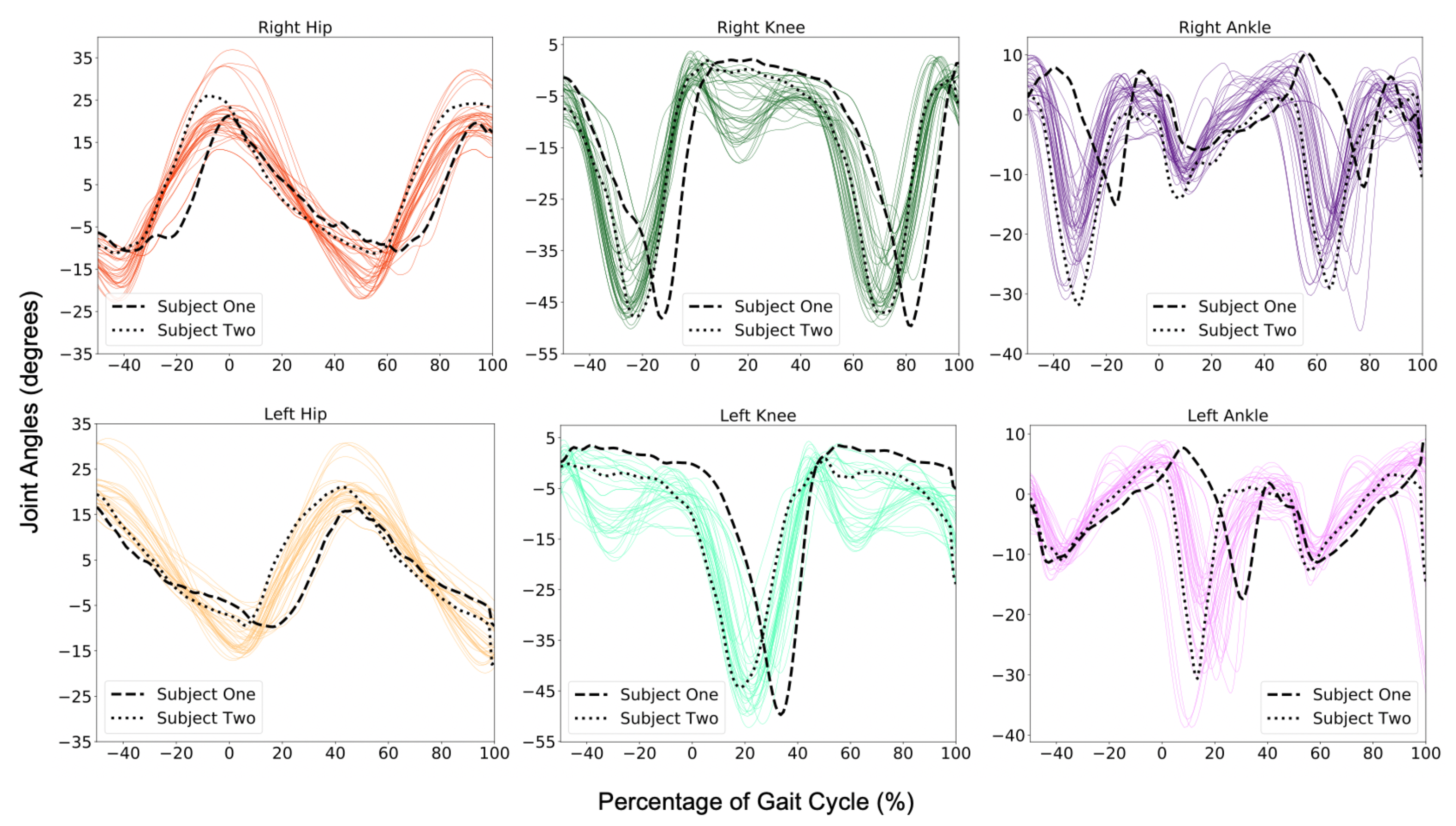
Joint angles are calculated using Equation (2) using biomechZoo and OpenSim’s marker set for five participants. The dashed lines represent the averaged joint angles for Subject One, and the dotted lines show the averaged joint angles for Subject Two. It is clear from this figure that both subjects have different ranges of motion during gait cycles (i.e., Subject Two has more ankle flexibility than Subject One), but still show a general pattern of gait. It is worth noting that the color scheme remains consistent throughout all other figures for each joint (e.g., right hip: red, left hip: orange, right knee: green, left knee: teal, right ankle: purple, left ankle: pink).
Figure 3.
Joint angles are calculated using Equation (2) using biomechZoo and OpenSim’s marker set for five participants. The dashed lines represent the averaged joint angles for Subject One, and the dotted lines show the averaged joint angles for Subject Two. It is clear from this figure that both subjects have different ranges of motion during gait cycles (i.e., Subject Two has more ankle flexibility than Subject One), but still show a general pattern of gait. It is worth noting that the color scheme remains consistent throughout all other figures for each joint (e.g., right hip: red, left hip: orange, right knee: green, left knee: teal, right ankle: purple, left ankle: pink).

Figure 4.
System overview illustrating the process from acquiring the data to exporting a model for gait recognition. The process begins by importing the data from either public databases [13,14] or our own OpenSim simulated data. The features, or joint angles, are extracted into a labeled data set that simultaneously analyzes the moments for each phase of gait, and cross-validation to create a test-split for the Gait Classification Model. After the Gait Classification Model has been loaded, different feature combinations are tested to yield the optimal feature combination (minimum joint angles) along with Grid Search to find the optimal parameters for an Evaluated Model to best predict phases of gait.

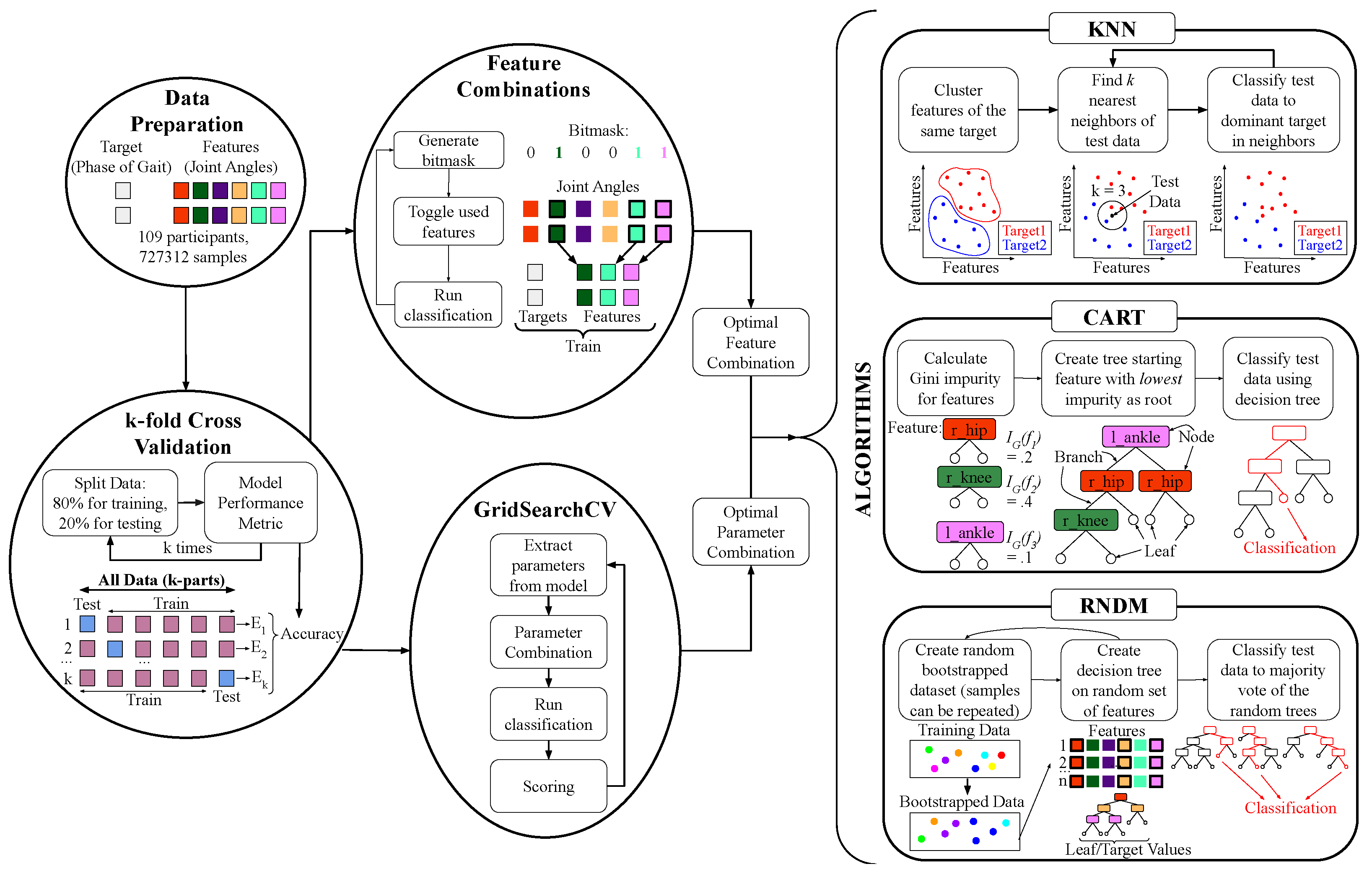
Figure 5.
Machine learning pipeline for the labeling, splitting, and classification of data to optimize the accuracy of the gait recognition model. The process begins with the preparation of data, where the target, or phase of gait, is tagged onto a feature set of joint angles. Before classification, the labeled data set is split between training and testing to reduce variance and support a more generalized performance metric of each algorithm. To optimize each algorithm, a feature split and parameter tuning is iterated through. Each feature and parameter combination is then run through the preferred machine learning algorithms.

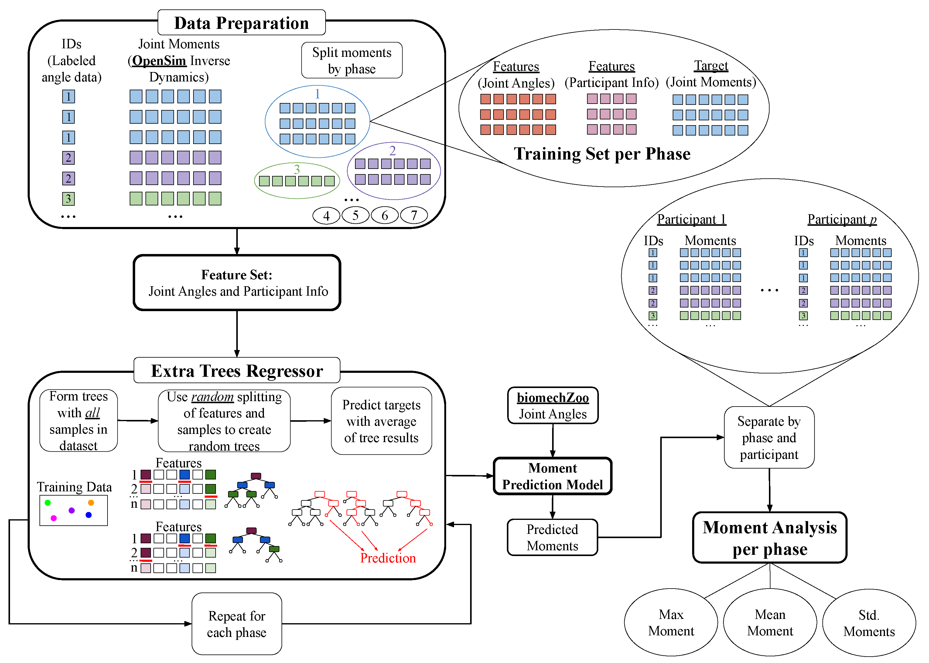
Figure 6.
Pipeline for creating a moment prediction model that categorizes phases of gait and participant information to yield the max, mean, and standard deviation for moments (Nm/kg). The data preparation process groups all of the joint moments, angles, and participant information by phase of gait. This feature set is then split randomly to ensure that the model does not rely heavily on any individual feature, and repeated 7 times for each phase of gait.

Figure 7.
Relationship between accuracy yielded from predicting phase of gait from joint angles and the combination of used features: right hip (red), knee (green), ankle (purple), left hip (yellow), knee (teal), and ankle (pink). It is important to note that if there is only 1 feature there is no way a tree can be formed, so there are no decision tree outputs for those feature combinations. This method to find the optimal feature combination, or feature reduction, demonstrates there is no need to monitor all 6 joints to result in a high phase of gait predictive model. See Table A6 for a numeric representation.

Figure 8.
The values as predicted by the Extra Trees Regressor (Figure 6) form predicted maximum moments (Nm/kg) for each joint. The average maximum moment required for the transition between each phase is plotted as a continuous line with the maximum for each phase based off of our subject pool. It is important to realize that every participant has a unique gait pattern, but the regressand, or outcome, yields a general approximation or trend for each phase. For numeric representations see Table A8. (a) Right hip. (b) Left hip. (c) Right knee. (d) Left knee. (e) Right ankle. (f) Left ankle.


Publisher’s Note: MDPI stays neutral with regard to jurisdictional claims in published maps and institutional affiliations. |
© 2022 by the authors. Licensee MDPI, Basel, Switzerland. This article is an open access article distributed under the terms and conditions of the Creative Commons Attribution (CC BY) license (https://creativecommons.org/licenses/by/4.0/).
Share and Cite
MDPI and ACS Style
Jung, E.; Lin, C.; Contreras, M.; Teodorescu, M. Applied Machine Learning on Phase of Gait Classification and Joint-Moment Regression. Biomechanics 2022, 2, 44-65. https://0-doi-org.brum.beds.ac.uk/10.3390/biomechanics2010006
AMA Style
Jung E, Lin C, Contreras M, Teodorescu M. Applied Machine Learning on Phase of Gait Classification and Joint-Moment Regression. Biomechanics. 2022; 2(1):44-65. https://0-doi-org.brum.beds.ac.uk/10.3390/biomechanics2010006
Chicago/Turabian StyleJung, Erik, Cheryl Lin, Martin Contreras, and Mircea Teodorescu. 2022. "Applied Machine Learning on Phase of Gait Classification and Joint-Moment Regression" Biomechanics 2, no. 1: 44-65. https://0-doi-org.brum.beds.ac.uk/10.3390/biomechanics2010006