
New Geometrical Modelling for 2D Fabric and 2.5D Interlock Composites


1
Faculty of Engineering, Lebanese University, Beirut 1002, Lebanon
2
Laboratory of Mechanical & Material Engineering, University of Technology of Troyes, 10420 Troyes, France
*
Author to whom correspondence should be addressed.
Textiles 2022, 2(1), 142-161; https://0-doi-org.brum.beds.ac.uk/10.3390/textiles2010008
Submission received: 13 January 2022
/
Revised: 13 February 2022
/
Accepted: 24 February 2022
/
Published: 7 March 2022
(This article belongs to the Special Issue New Research Trends for Textiles)
Abstract
:A new geometrical modeling tool has been developed to predict the elastic stiffness properties of 2D orthogonal and 2.5D woven interlock composites. The model estimates the change in performance due to changes in the ordering weaving parameters of the 2.5D weave architecture. Analysis results were validated compared to other models developed in published articles and the literature. Numerical analysis was performed to evaluate the accuracy of the results from the proposed models. These results demonstrate the effectiveness of the models presented by comparisons with experimental results, showing that the model could replicate the mechanical behaviors of 2D fabric and 2.5D interlock composite laminates for predicting 2D textile structures and 2.5D interlock composites with different types, shapes, and conditions. The model presented in this paper is able to replicate the behavior of woven composites of fiber reinforced with various types.
1. Introduction
Woven compounds are being increasingly considered for lots of applications because they provide ease in making complex geometries, but the mechanical properties of the different weave material supports are less visible than non-woven (angle-ply) laminates [1]. Note that there is no mathematical modelling of structural fiber-reinforced composite structures, though one measurement was obtained here using estimates in which woven fibers were formed from two orthotropic unidirectional fiber results in a curved twist using a weave. Recently, there has been in increased focus on exploring integrated and complete mechanical properties and methods of textile composites tested for uniaxial or biaxial tension, pressure, flexibility, and short-beam cutting [2,3,4,5]. Various analytical techniques have been developed to predict the elastic properties of representative volume elements (RVEs) of textile composites that include 2D and 3D weave composite. Woven composites can provide a potential solution to the basic limitations of traditional laminated composites: delamination and production that requires more workers. The addition of binder yarns provides through-thickness reinforcement, leading to highly advanced interlaminar materials and fabric binding to allow near-net-shape preforms to be woven and handled [6].
However, apart from these benefits, the use of 2.5D woven compounds is very limited in niche applications. One of the main reasons for this is the lack of predictive numerical tools, which limit their use in the early stages of design. Another method of production is to cut a simple three-dimensional weave, consisting of two two-dimensional (2D) fabrics connected by twisted loops of yarn, to form a ‘hairy’ fabric. These 2.5D fabrics are then coated with epoxy resin in a standard way, laminated, and treated with autoclave [7]. Woven Composites (2.5D-WC) not only have a higher delamination resistance compared to 2D laminated composites, but also have a simpler structure than 3D textile composites. Recently, most parts in the aero-engine sector, namely fan/compressor blades and casing, were made using 2.5D-WC [8].
1.1. Objective
The purpose of this paper is to introduce new content and a new, simple geometrical model for analyzing the mechanical properties of woven composites, i.e., 2D and 2.5D. In addition, the model will estimate the change in performance due to changing the weaving parameters that dictates the 2.5D weave architecture about the elastic properties; this is discussed in detail. Finally, important conclusions are reached.
An effective recursive algorithm, a matrix solidification method, is designed for multi-layer media that is usually anisotropic. This algorithm has the efficiency and calculation of the standard transmission matrix method and is unconditional in terms of a high frequency calculation system and layer thickness. In this algorithm, the stiffness (compliance) matrix is calculated.
This algorithm allows researchers and end users to calculate the durability and compliance matrix of any woven compound material, of any type, shape, or thickness, while saving time and cost in finding the right solution.
This paper introduces a geometric modeling tool to predict the expandable stiffness features of 2.5D woven orthogonal interlock composites. The model is able to reproduce the behavior of woven composites formed by different fiber-reinforced types.
1.2. State of the Art
Various analytical techniques have been developed to predict the expansive properties of volume representation (RVEs) of textile composites that include 2D and 2.5D weave composites. Bogdanovich and Pastore [9], Whitcomb et al. [10], and Potluri and Thammandra [11] have conducted a complete review of the topic. Based on stiffness averaging and rigidity ratio, Ishikawa and Chou [12,13,14] managed a two-orthogonal set of fabric compositions such as laminate with two laminae placed at 0/90 position. They proposed different models for predictable expansion, such as (1) a mosaic model (where fiber continuity and retraction was left), (2) a crimp model (where fiber continuity and undulation geometry were defined using the functions of -trigonometric), and (3) bridge coupling model (rigid or compliant dimensions in two orthogonal directions and suitable for satin weave combinations). Naik et al. [15,16] analyzed fiber retreat to the two orthogonal directions and used detailed trigonometric functions to extend the crimson models of Ishikawa and Chou (i.e., parallel two-dimensional series models and series-parallel models) to test expandable structures different combinations of PWF. Saka and Harding [17] and Carey et al. [18] developed rectilinear and sinusoidal crimp models to predict expansion structures using the classic laminate plate theory applied in the context of an expandable base and using the same power system. Tong et al. [19] take fiber as a curved rod based on stretch elastic or shear base in a woven composite structure and present a curved bark model to investigate the impact of fiber flexibility on the strength of woven composite material based on the concept of classical laminate plate theory. Kollegal and Sridharan [20] employed hierarchic works to determine the original curved profile of the strings and plate displays and introduced the micro-plate model for PWF analysis.
A significant amount of research was performed using the principles of differential stress [11,21] or FE (FEA) analysis [22,23,24] to analyze the expandable tracts of woven compounds and a detailed stress field across the RVE from the limited equipment. Regarding basic properties, in order to produce FE models, precise vertical segments or continuous mathematical functions are used to demonstrate in detail the ideal PWF geometry and to represent the thread path and cross section shape.
Mesoscopic simulations of transverse compaction have attracted recent interest. Geometric modeling methods have been developed using fabric matching software such as TexGen [25,26] or WiseTex [27,28], which have been used in various articles [29,30,31,32,33]. Multi-chain digital element-based methods have also been used [34,35,36,37,38]. Green et al. [39,40] proposed a numerical procedure for creating mesostructural geometric models in simulated fabrics by combining appropriate TexGen models with multi-chain digital materials. Nguyen et al. [41] followed the method developed by Hivet and Boisse [42] to produce mesostructural geometric models of 2D woven fabrics to mimic the opposite combination. Numerical simulations of hypo elastic material based on fiber rotation were well matched to experiments. Alternatively, based on the discrete homogenization method, Goda et al. [43] and Rahali et al. [44] can reproduce the functional properties of 2.5D machines and 3D interlock textiles. Zhang et al. [45] developed a model based on the optical aspect ratio to predict mechanical responses and failure location under uniaxial and biaxial loading.
However, these methods are based on appropriate geometrical models, therefore cannot explain mesostructural changes in fiber structure, i.e., a detailed study of how fibers degenerate under bonding. Consideration and simplicity are often needed in numerical matching, which reduces calculation costs, facilitates the modeling process, and provides computer estimations. However, this simplification may prevent the investigation of other events occurring in real systems, especially in the case of mesoscopic and microscopic disorders.
Specific studies of mesoscopic transformation of fibrous reinforcement can also be performed with minimally invasive imaging such as X-ray micro-computed tomography (Micro-CT). With this process, it is possible to measure, model, and analyze the geometric structure of fiber cables. Desplentere et al. [46] and Schell et al. [47,48] were among the first to demonstrate the power of Micro-CT to show the geometric features of 3D fabrics on a mesoscopic scale. In Pazmino et al.’s study [49], the geometric features are directly measured by the fiber pulse from small tomographic images to read a single layer of 3D non-crimp woven fabric. Naouar et al.’s [50,51] mesostructural geometry models successfully reconstructed 2D woven fabric and 3D orthogonal fabric from small tomographic images. Wang et al. [52] studied longitudinal compression and the Poisson number of fiber cables followed a similar pattern. Badel et al. [53] performed both numerical simulations and tomographic analyzes of 2D woven fabrics under biaxial tension and in-plane shear deformation.
Combined with digital volume integration, Mendoza et al. [54] developed a mathematical model for the distortion of woven compounds, which was recently used to measure the flexibility caused by the production process [55]. However, no research studies to date have reported on the analysis of variables based on meso-structural models of fiberglass fabrics separated by these simplified methods at different levels of assembly.
Methodology:

2. Geometrical Modelling
2.1. 2D Fabric
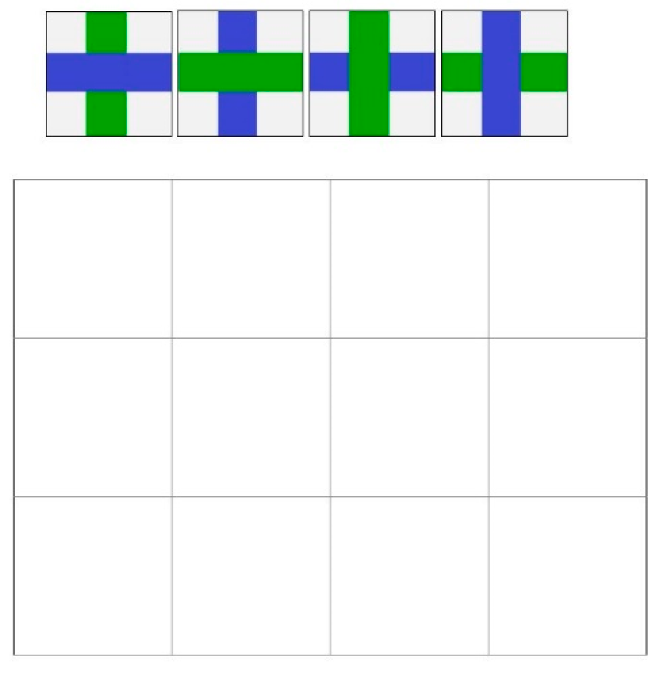
The user—whether a student or a fellow researcher—can themselves design a fabric composite. To construct the whole structure of composite as he or she likes from the beginning and to make the whole process “user friendly”, the process took the shape of building a puzzle by a simple “click and drop” game as shown in the figure below (Figure 1).
As 2D woven fabrics are made by interlacing yarns in a weaving loom, yarns are divided into two components: one called the warp, running along the length of the loom, and the other is the weft, running in the cross direction. The woven structure is characterized by orthogonal linking of two sets of threads, called warp and weft yarn. The warp threads are aligned with the direction of the fabric leaving the weaving equipment, which is also called the warp direction. As shown in Figure 2, 2D woven fabric has two yarn sets as warp (0°) and filling (90°) and interlaced to each other to form the surface.
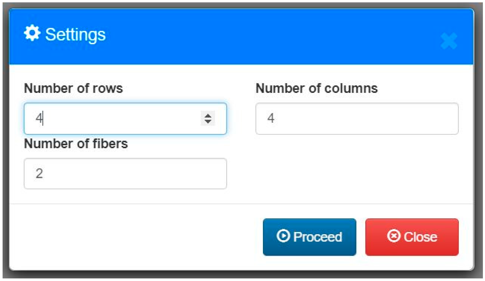
To start from the beginning, the user is free to choose the settings of the puzzle in each dimension, i.e., number of columns and rows, and the number of fibers, as shown in Figure 3.
The next step is to construct the geometry as desired and shown in the following examples in Figure 4, Figure 5, Figure 6 and Figure 7.
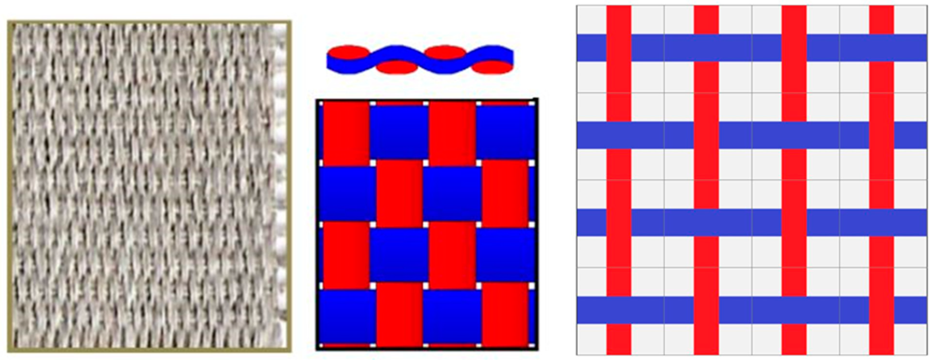
2.1.1. Plain Weave Fabric [1/1]
Plain weave is a very common and very strong basic weave where each warp fiber passes alternately below and above each weft. The fabric is symmetrical and has good stability and logical porosity. However, they are the most difficult to weave, and the high quality of fiber crimp offers lower mechanical features compared to other weaving styles.
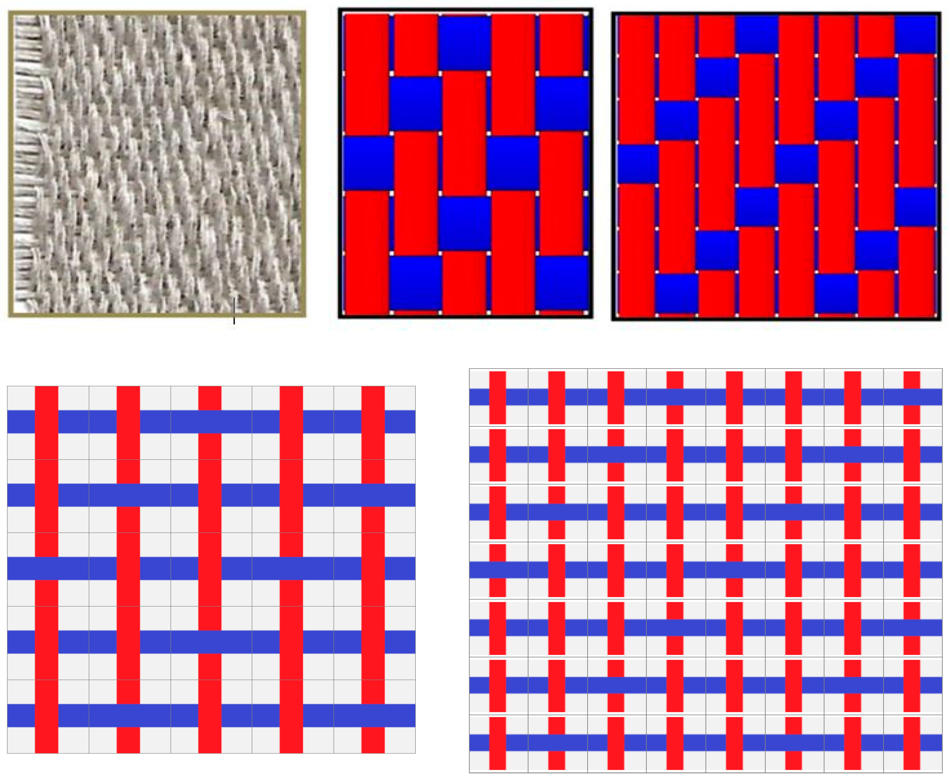
2.1.2. Twill [2/1, 3/1]
Twill is a type of textile weave with a pattern of corresponding diagonal ribs. It can be seen by observing the presence of diagonal lines that are pronounced along the width of the fabric. It has a higher resistance to cracking than plain weave because it has fewer wires that connect to each area, hence the greater the internal flow rate. In addition, two strings will carry the load when the fabric is torn.
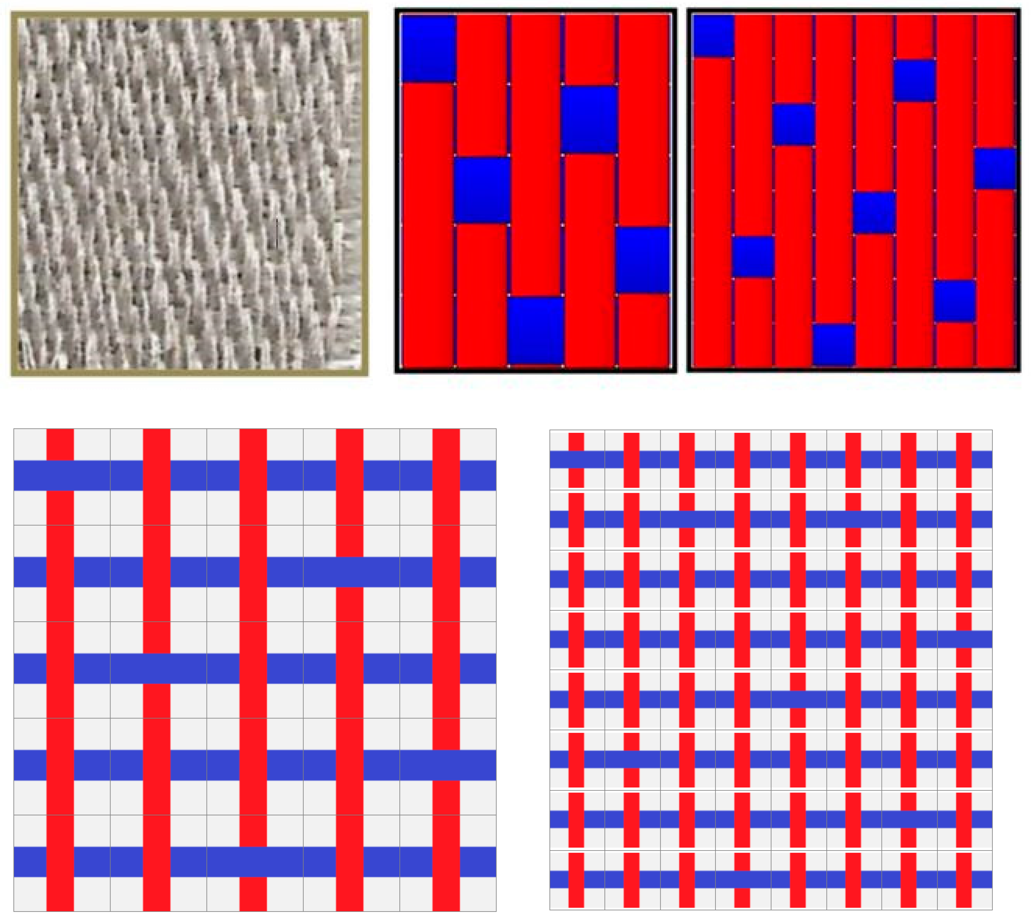
2.1.3. Sateen/Satin [5-end, 8-end]
Sateen is a fabric that usually has a shiny surface and a hidden back, one of the three basic types of fabric weaving, seamless weaving, and twill. Four or more full-length or single-stranded strands floating over a straight rope, and four straight strands floating on a single weft thread indicate satin weaving. Floating strings are missed interfaces, where the warp thread lies on the weft in a satin with a straight face and where the weft thread lies on straight strands on satin with a weft face.
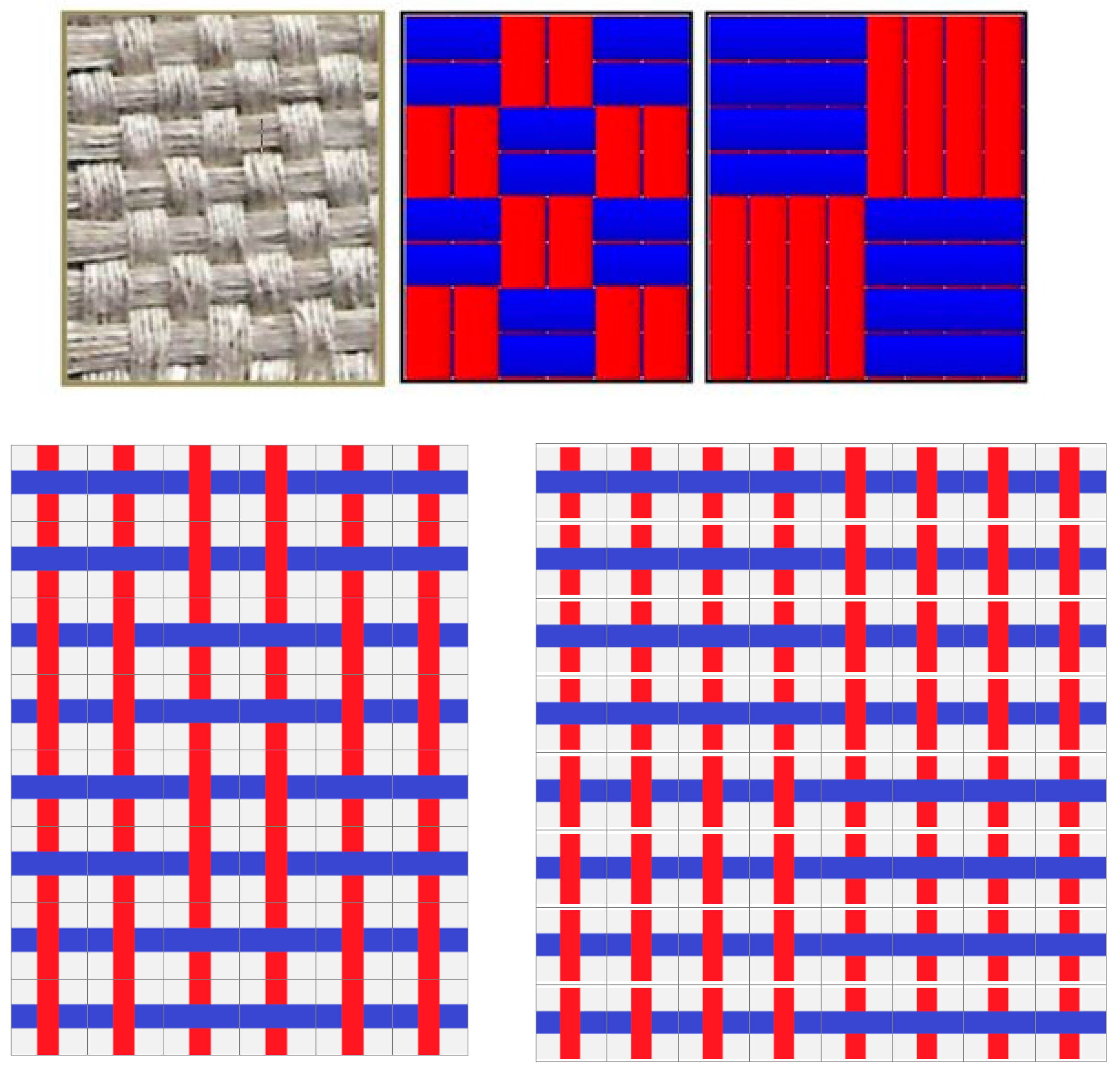
2.1.4. Basket Weave [2/2, 4/4]
Basket weave is known also as Hopsack and Matt Weave. Hopsack weave, a variant of plain weave, uses two or more warp and/or two or more weft fibers joined as a single thread. This weave is obtained by doubling or repeating the combined points of a plain weave in both the direction of the wrap and weft. These fabrics are made of two or more strings placed in the same shed. The stitching pattern is similar to a plain weave, but two or more strands follow the same parallel pattern. Fabrics designed by Matt are flexible and cannot wrinkle as there are a few cutters that are a square inch. Fabrics look flatter than conventional weaving fabrics. However, longer floats are more flexible. Matt fabric has great anti-tear properties. Matt’s design tends to offer more smooth fabrics. For a repetitive Matt weave size, the warp numbers and weft threads are equal.
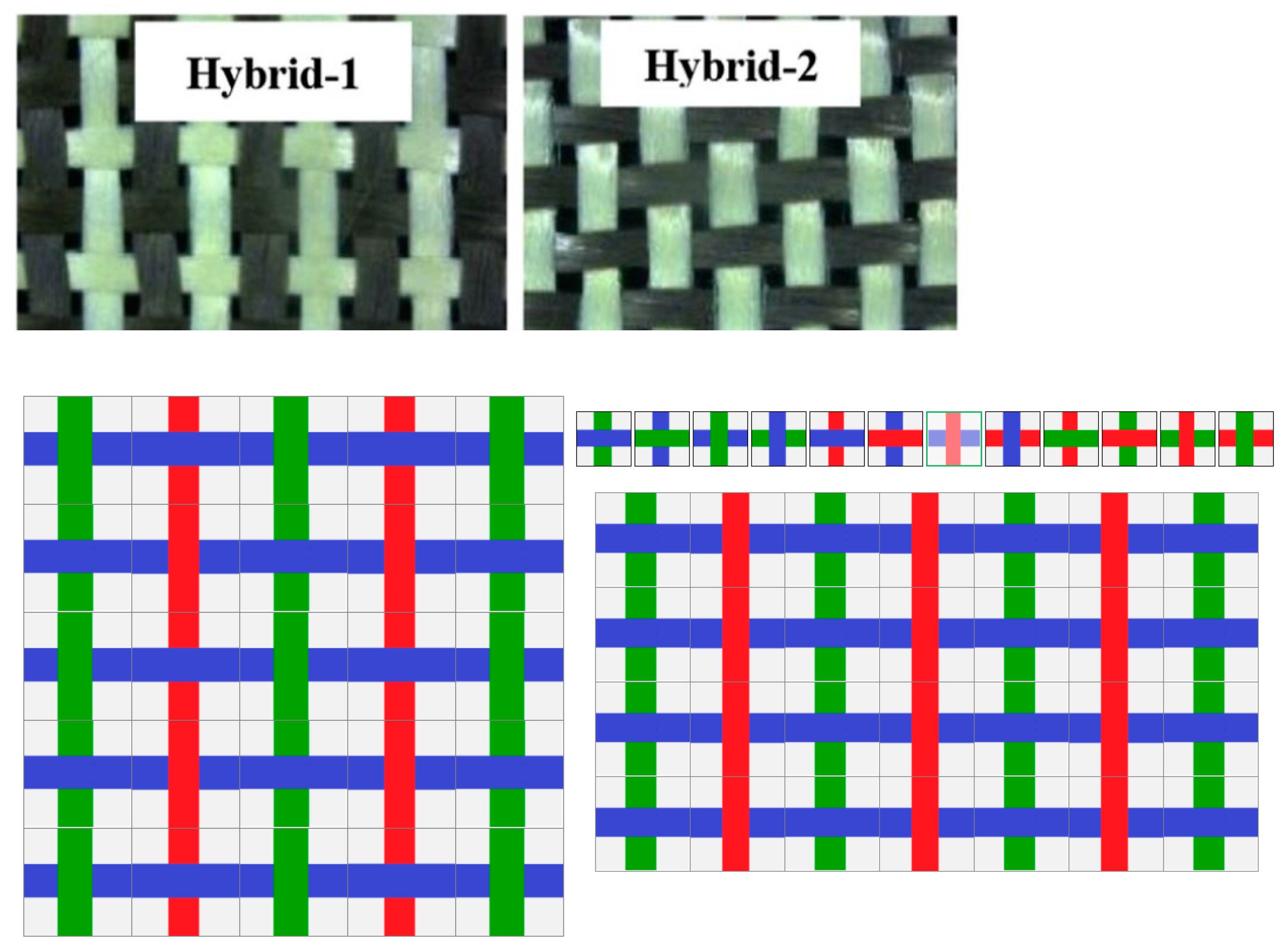
2.1.5. 2D Fabric Hybrid Composites
Hybrid yarns are where two or more fibers are brought together to combine the performance and aesthetic of both, as shown in Figure 8. Although environmental concerns are encouraging many manufacturers to focus on the use of a single fiber, there are still and will remain reasons for bringing fibers with different qualities together, particularly for performance and health and safety applications.
2.2. Interlock Composite 2.5D
The 2.5D, or so-called 3D, interlock composite is a special fabric combination in which mechanical properties are closely related to its structure. The geometry of the interlock is complex and the number of possible structures is infinite. Fabric architecture depends on the extraction, crimp, and size of the fiber fibers. It is made up of a system of two woven and interconnected yarns, straight yarns, and weft (or filling) yarns. Interlacing caused by bending is called “tow crimp”.
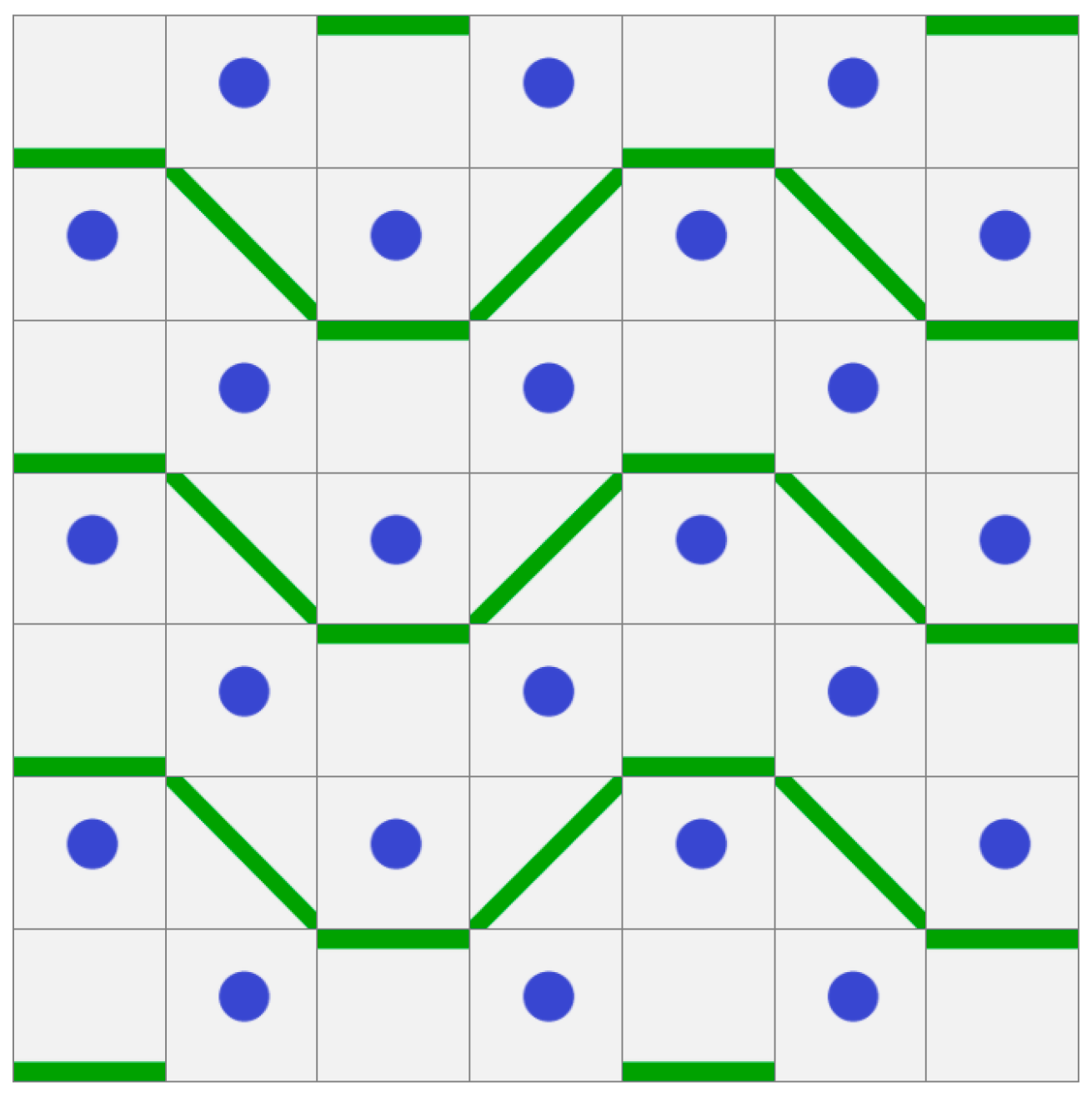
The shapes in the “puzzle” represent the filler element and the bounder (interlock fiber) of the structure, as shown in the figure below (Figure 9), in 2D view.
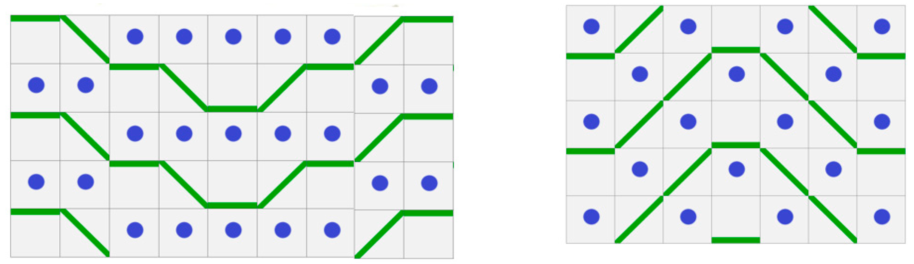
2.5D angle closing fabrics can be divided into two types: thick fabrics and fabrics from layer to layer. This type of combination is characterized by its intricate structure. The cell unit consists of a warp weaver and weft fibers attached to 90° plane (xy) (Figure 10 and Figure 11). A 2.5D angle woven joint includes warp that binds to warp straight cords by attaching warp threads. Warp wires can be tied to different depths where different layout arrangements could be used to produce a wide range of these types of compounds. Tight fabric is a multi-layered fabric where warp weavers move from one piece of fabric to another, holding all the layers together. The layer-to-layer fabric as shown in Figure 10 is a multi-layer fabric that the warp weavers move from one layer to the nearest layer and back. A collection of warp woven together holds all the layers of fabric. In addition, complex geometry as shown in Figure 11, fractional volume fraction, cable volume, and inclination angle of warp strands are not able to allow the structural properties of specific applications. In other words, designers can replicate the efficient performance of fabrics for the necessary mechanical properties.
- 1
- Layer to Layer Angle Interlock
- 2
- Through the Thickness Angle Interlock
2.3. Construction Testing
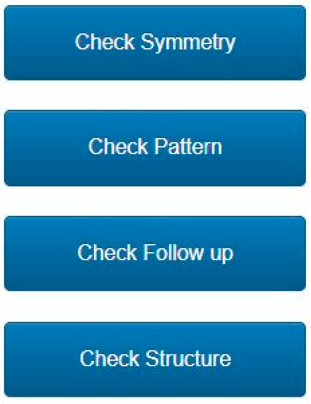
Tests should be performed as shown in Figure 10 and Figure 11 to validate the shape suggested by the user. These tests are:
- -
- Follow up test.
- -
- Pattern test.
- -
- Symmetry test (not obligatory).
These tests obtained by logical geometrical construction of the 2.5D interlock structure are as constrains that define whether the design (structure) from the user is valid–applicable—as shown in Figure 10.
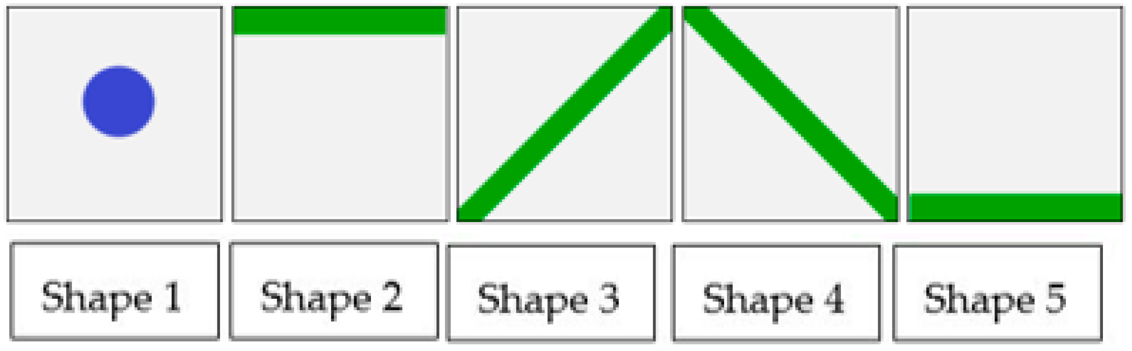
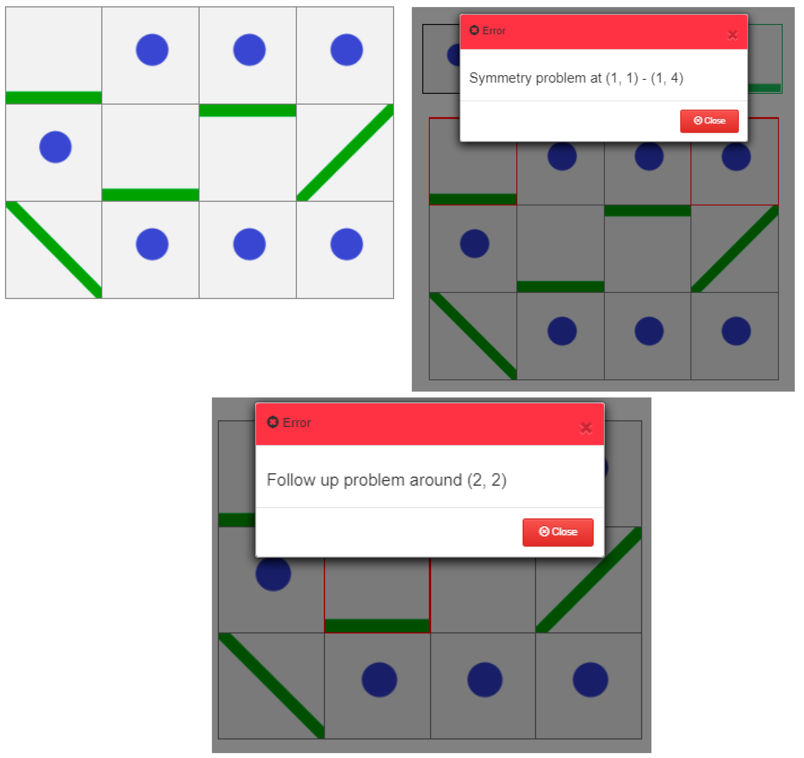
As named, the function of the tests are to check if there is a continuity of structure and if there is a possibility to add a shape in the puzzle as shown in Figure 12. For example, Shape 3 cannot be similar to Shape 2′s incident and reflected interlock at the same time. The puzzle should be symmetrical if the user is constructing a symmetrical shape. If not, the test to check symmetry can be deactivated. Shapes 2, 3, and 4 cannot be repeated vertically. Shapes 2 and 4 cannot be repeated horizontally. Shapes 2 and 4 should be separated only by Shape 3. Shape 3 cannot follow Shape 1 or 2. At least one instance of Shape 1 should separate Shapes 2 and 4 horizontally. In addition, there are other structural and geometrical conditions and boundaries related to the shape.
Note that all these conditions/boundaries are tested automatically by the JavaScript code created by the author.
Moreover, if there is any structural mistake made by the designer (user) the code will identify the mistake with the relation of the mentioned tests. In addition, the code will specify exactly the place of the error with the messages: “Pattern problem at column 2—Follow up problem at (2,2)—Invalid structure” for the designer have to reshape its structure to continue and the sentences “No pattern problem—No follow up problem—Valid structure”, as shown in Figure 13
2.4. Analytical Modelling
First, the user should fill fibers and matrix parameters such as Young’s and shear modulus (Ei,Gi) and fiber volume fraction (Vf) as shown in Figure 14 as a user interface to the analytical modelling.
Then, to calculate the characteristics of the key elements and the contribution rate, they make a macroscopic layer and subsequently the whole unit cell. The current approach creates expressions at the micro level with the aim of calculating more representative volume fractions of a group of elements to the layer to improve the elastic stiffness speculation compared to existing analytical modeling methods that use the 2.5D woven composite as a composite component containing layers of unidirectional elements (which are fibrous tows encased in resin). The new modelling approach creates expressions that discretize the unit cell into elements
To calculate the macroscopic stiffness of the whole unit cell, it must be broken down or discretized to the microscale. The microscale looks at the individual elements that make a cell and then the layers that make up the macroscopic unit cell. Therefore, the unit cell undergoes the first level discretization into layers, then the second level discretization into the individual elements that make up the layer. An element can be an individual, filler, binder, or matrix region within a layer. Having determined the stiffness of each element, the stiffness of whole row can be found. Once the stiffness of all rows is known, the model formulates and calculates the stiffness of the whole unit cell and finally outputs the elastic constants. The prediction of the unit cell or macroscopic stiffness begins with the calculation at the micro scale (the constituent elements within a cell).
The algorithm applied is as follows:

The fiber matrix (S) strength can be easily calculated. In the pocket of a pure resin matrix, it is generally regarded as isotropic substances. When the elastic modulus and Poisson’s ratio of resin matrix are given, it is easy to determine its basic relationship. It is easy to obtain their compliance matrix in the local material coordinate systems (1- 2- 3) to (x- y- z) by inverting their stiffness matrix (Sij) as shown in Equations (1) and (2).
Each type of cell unit consists of two types of elements, namely fiber and a pure resin matrix. First, the lamina compliance matrix was calculated. Like most micro-mechanical models, the fibers and the resin matrix assume transversely isotropic, and both of them assume to be linearly elastic in the model. In order to achieve the elastic properties of the composites, the Chamis-proposed fiber-matrix ROM was selected to compute the engineering elastic constants. The Chamis micro-mechanical is a widely used and reliable model, providing an equation of all five independent structures that stretch like this [56]:
where Vf is the fiber volume fraction, Ef11 is the Young’s elastic modulus of the fiber in principle axis 1, Ef22 is the Young’s elastic modulus of the fiber in principle axis 2, Gf12 is the longitudinal shear modulus of the fiber, Gf23 is the transverse shear modulus of the fiber, νf12 is the primary Poisson’s ratio of the fiber, and Em, νm, and Gm represent the Young’s elastic modulus, Poisson’s ratio, and shear modulus of the matrix, respectively.
E11 = VfEf11 + VmEm
E22 = E33 = Em/(1 − √Vf (1 − Em/(Ef22)))
G23 = Gm/(1 − √Vf (1 − Gm/(Gf23)))
G12 = G13 = Gm/(1 − √Vf (1 − Gm/(Gf22)))
ν23 = Vfνf23 + Vm (2νm − ν12 (E22/E11))
ν12 = ν13 = νm + νf (νf12 − νm)
The compliance matrix of the fiber can be easily calculated. For the pure resin matrix pocket, it is generally regarded as isotropic material. When the elastic modulus and Poisson’s ratio of resin matrix are given, it is easy to determine its basic relationship.
After that, we can obtain the stiffness in the global coordinate system by transforming the stresses and strains with the generalized transformation matrix as the next form:
where k is the number of unit cells in the Puzzle structure and the angle defined as the cosines of the angle between the axes of the local and global coordinate systems before and after rotation:
where θ is the angle of weaving for the yarns.
[Cb] = [T]kT[C]k[T]k
c = Cos (θ)
s = Sin (θ)
A unidirectional cell falls under the orthotropic material category. As the cell is thin and does not carry any out-of-plane loads, one can assume plane stress conditions for the cell.
Therefore, assuming σ3 = 0, τ23 = 0, and τ31 = 0, calculation of element contribution is required so that the stiffness of the whole cell can be calculated as well as the overall unit cell stiffness. In our case, the contribution is related to the percentage in volume of the bounder (interlock fiber) with reference to the matrix volume (for example 30% bounder, 70% resin).
where [Cb] and [Cm] are the bounder and resin stiffness matrix in the global coordinate system, respectively, p is the percentage in volume of the bounder and resin in the composite structure, and k is the number of element in the whole structure.
Mij = (p) CbKij + (1 − p) CKmij
Calculating the total matrix/row by summation of matrices (series summation) as shown in Equation (14):
where n is the number of rows in the puzzle and [Mi] are the inverse of matrices found in Equation (14).
The final step is the summation of the found matrices in column and in rows as shown in Equation (15):
where m is the number of columns in the puzzle and [Mt-1i] are the matrices found in Equation (15).
3. Materials
3.1. 2D Fabric
To ensure the effectiveness of this model based on this work. In comparison between current results modeling, experimental data, and previously developed multi-scale modelling, four different examples are generated. As studies, different mechanical features are considered and results are released. Examples were chosen from the specimens studied by J.J. Xiong and his co-workers [57] to calculate the engineering elastic constants of 2D Fabric Woven composites.
The composites studied in this section are the following:
- E-glass/epoxy—I;
- E-glass/epoxy—II;
- T300/epoxy;
- EW220/5284.
The fabric specifications and mechanical properties of the above four kinds of textile composites are listed in Table 1
3.2. 2.5D Interlock
The composites are made from carbon fibers T300J and resin matrix RTM6 (Table 2). Two examples were chosen from the specimens studied by Hallal and his co-workers on 3SHM (3 stages homogenization method) [58]. The architecture of these composites involves only warp weaver yarns and weft straight yarns, as shown in Figure 10 and Figure 11. The REV of the composite-H2 is composed of 6 warp yarns and 12 weft yarns, while the REV of the composite 71 is composed of 3 warp yarns and 24 weft yarns. The REV of composite 69 contains 6 warp yarns and 6 weft yarns. Warp yarns have a mean inclination angle equal to 29° for the linear longitudinal part of weft yarns. The warp yarns have a linear plus undulated longitudinal parts and a flattened elliptical cross-section. They are interlocked with weft yarns in two steps. Undulated parts have a mean inclination angle equal to 24° for H2 and 12° for 71. The weft yarns have a linear longitudinal part while its cross-section is a flattened ellipse. In addition, the fiber volume fractions in both warp and weft yarns is taken equal to 0.6. Table 2 shows the mechanical properties of carbon fibers and matrix. Carbon fibers assumed transversely isotropic material, which gives the following assumption:
4. Results and Discussion
With the purpose of validating the developed modeling technique, the results were compared with experimental data published in the open literature. A comparison between the results of the present modeling, experimental data, and previously developed multi-scale modeling was conducted. As case studies, different mechanical properties were considered, and the results are shown in Table 3, Table 4 and Table 5, each of which shows a clear comparison between the experimental results and the presented model.
For example, Table 3 shows the comparison of longitudinal and Young’s moduli between four different materials and fibers studied by J.J. Xiong [57]. On the other hand, Table 4, Table 5 and Table 6 show a clear comparison for the section of 2.5D interlock composite with its different types.
4.1. 2D Fabric
As shown in Table 3, the comparison was focused on tension moduli from the specimens studied by J.J. Xiong and his co-workers [57]. The method present accurate and precise values with the percentages of error varied from 0.44% for longitudinal Young’s modulus Ex, in E-glass/epoxy—II experiment up 1.91% for EW220/5284.
4.2. 5D Interlock
The following table presents the results found by a previous analytical model from the reference validation mentioned earlier
The comparison was made to the engineering properties found using the code. A few notes should be taken into consideration: The model does not have curvature shape between Shapes 2, 3, and 4. The structure is in the coordinate system (x, y) by the reference. The dimensions of fiber are considered to be a tube shaped form and not elliptical. By comparing the result, we see that there is a validation to the code and the new model with a marginal error due to the curvature shape missing and the real/theoretical shape relation between the numerical, analytical, and geometrical model. It was observed from Table 4 that the Young’s modulus in direction 2 is the most accurate parameter, up to 1% in comparison 3SHM found in Hallal [58], and that the maximum average error is shown for the Young’s modulus in direction 1 with 10% of error. From Table 4, the percentage of error of transverse Young’s modulus is much higher than for the longitudinal Young’s modulus, with a value of 4.13% as the percentage of error of longitudinal Young’s modulus was 0.614%. In addition, the percentages of error for shear modulus in Table 4 and Table 5 were 1.12% and 1.21%, respectively. Finally, from Table 6, the percentage of error of transverse Young’s modulus was also much higher than for the longitudinal Young’s modulus, with a value of 5.07% and the percentage of error of longitudinal Young’s modulus was 1%. The percentage of error for shear modulus in Table 6 was 1.31%.
In addition to the high accuracy level of the current modelling technique, the very short runtime required of the modelling renders the developed multi-scale modelling as a cost-effective computational tool for estimating the Young’s moduli of laminate composites. The results showed that the present model could be used to effectively evaluate the elastic properties for laminate composites.
5. Conclusions
A geometrical-modelling tool has been presented to predict the elastic stiffness characteristics of 2D fabric and 2.5D woven interlock composites with the ability to assess change in performance as a consequence of altering weaving parameters. The models presented in this paper are able to reproduce the behavior of woven composites formed by different fiber-reinforced types. This approach has been validated against experimental data produced independently of this work for orthogonal interlock weaves and compared to existing modelling approaches. The present model performs better in all predictions compared to the existing modelling efforts. Good agreement was observed among numerical results, with small differences in the longitudinal strains, as shown in the results section that the shear modulus was the most accurate parameter up to 1% in the 2.5D interlock section, while the error in 2D fabric section was lower with values such as 0.44% in tension moduli. As for the longitudinal Young’s modulus, the maximum average error is shown with 10% but with an average percentage of error of transversal strains of 4%. This may be due to a lack of precision in the mechanical properties of the components, i.e., the fibers, which are used as input data. The percentage is related to the lack of an accurate and precise database structure of the used material, but it shows a great ability to use the algorithm.
The suggested hypotheses are the simplest that can be applied for determining the engineering data with all required information, and specifications from the user are presented in a “user friendly” form that can make studying and searching a new level of excitement and interactivity. As shown in the methodology section, applying the algorithm is easy and simple. All this research can be accessed easily with all its codes and models, along with its regulations and explanations needed. Working on these codes will eliminate the hard work caused by the computational efforts using software such as Abaqus or Ansys, etc.
At any given time, the user can calculate required forces to have a known deformation or to predict the deformation for a known force; in addition, they would have easy access to all engineering properties such as stiffness or compliance matrices. A future scope is now set in each section to have more research and data analysis by using these codes and models without any super computers and losing time, money, and effort. Any researcher can now find the optimum set of materials for all levels of woven composites materials (2D Plain weave, Twill, Satin, or Basket), along with altering materials for 2.5D interlock composites such as layer to layer or through the thickness angle interlock. The model works best on other types of combinations, and further analysis and evaluation of the models is required. The introduced framework may apply to other fiber conditions as part of a fiber volume, but these conditions will require further development.
Author Contributions
R.Y.: Methodology and Supervision, P.L.: Data and spelling, M.A.K.: Writing, calculating, programming and analyzing. All authors have read and agreed to the published version of the manuscript.
Funding
This research received no external funding.
Institutional Review Board Statement
Not applicable.
Informed Consent Statement
Not applicable.
Data Availability Statement
Not applicable.
Conflicts of Interest
The authors declare no conflict of interest.
References
- Ghlaim, D.K. Woven factor for the mechancial properties of woven composite materials. J. Eng. 2010, 16, 4. [Google Scholar]
- Ishikawa, T.; Matsushima, M.; Hayashi, Y.; Chou, T.W. Experimental confirmation of the theory of elastic moduli of fabric composites. J. Compos. Mater. 1985, 19, 443–458. [Google Scholar] [CrossRef]
- Tan, P.; Tong, L.Y.; Steven, G.P.; Ishikawa, T. Behavior of 3D orthogonal woven CFRP composites. Part I. Experi-mental investi-gation. Composites A 2000, 31, 259–271. [Google Scholar] [CrossRef]
- Botelho, E.C.; Figiel, L.; Rezende, M.C.; Lauke, B. Mechanical behavior of carbon fiber reinforced polyamide compo-sites. Com-pos. Sci. Technol. 2003, 63, 1843–1855. [Google Scholar] [CrossRef]
- Wang, Y.J.; Zhao, D.M. Effect of Fabric Structures on the Mechanical Properties of 3-D Textile Composites. J. Ind. Text. 2006, 35, 239–256. [Google Scholar] [CrossRef]
- Greena, S.D.; Matveevb, M.Y. Mechanical modelling of 3D woven composites considering realistic unit cell ge-ometry. Compos. Struct. 2014, 118, 284–293. [Google Scholar] [CrossRef] [Green Version]
- Wvan, A.; Vuure, J.; Ivens, A.; Verpoest, I. Mechanical properties of composite panels based on woven sand-wich-fabric preforms. Compos. Part A Appl. Sci. Manuf. 2000, 31, 671–680. [Google Scholar]
- Song, J.; Wen, D.W. Fatigue life prediction model of 2.5D woven composites at various temperatures. Chin. J. Aeronaut. 2018, 31, 310–329. [Google Scholar] [CrossRef]
- Bogdanovich, A.E.; Pastore, C.M. Mechanics of Textile and Laminated Composites, 1st ed.; Chapman & Hall: London, UK, 1996. [Google Scholar]
- Whitcomb, J.; Noh, J.; Chapman, C. Evaluation of Various Approximate Analyses for Plain Weave Composites. J. Compos. Mater. 1999, 33, 1958–1980. [Google Scholar] [CrossRef]
- Potluri, P.; Thammandra, V.S. Influence of uniaxial and biaxial tension on meso-scale geometry and strain fields in a woven composite. Compos. Struct. 2007, 77, 405–418. [Google Scholar] [CrossRef]
- Ishikawa, T.; Chou, T.-W. Elastic Behavior of Woven Hybrid Composites. J. Compos. Mater. 1982, 16, 2–19. [Google Scholar] [CrossRef]
- Ishikawa, T.; Chou, T.W. Stiffness and strength behavior of woven fabric composite. J. Mater. Sci. 1982, 17, 3211–3220. [Google Scholar] [CrossRef]
- Ishikawa, T.; Chou, T.W. One-dimensional micro-mechanical analysis of woven fabric composites. AIAA J. 1983, 21, 1714–1721. [Google Scholar] [CrossRef]
- Naik, N.K.; Shembekar, P.S. Elastic Behavior of Woven Fabric Composites: I—Lamina Analysis. J. Compos. Mater. 1992, 26, 2196–2225. [Google Scholar] [CrossRef]
- Naik, N.K.; Tiwari, S.I.; Kumar, R.S. An analytical model for compressive strength of plain weave fabric composites. Compos. Sci. Technol. 2003, 63, 609–625. [Google Scholar] [CrossRef]
- Saka, K.; Harding, J. A simple laminate theory approach to the prediction of the tensile impact strength of woven hybrid composites. Composites 1990, 21, 439–447. [Google Scholar] [CrossRef]
- Carey, J.; Munro, M.; Fahim, A. Longitudinal Elastic Modulus Prediction of a 2-D Braided Fiber Composite. J. Reinf. Plast. Compos. 2003, 22, 813–831. [Google Scholar] [CrossRef]
- Tong, L.Y.; Tan, P.; Steven, G.P. Effect of yarn waviness on strength of 3D orthogonal woven CFRP composite ma-terials. J. Reinf. Plast. Compos. 2002, 21, 153–173. [Google Scholar] [CrossRef]
- Kollegal, M.G.; Sridharan, S. A Simplified Model for Plain Woven Fabrics. J. Compos. Mater. 2000, 34, 1756–1786. [Google Scholar] [CrossRef]
- Sheng, S.Z.; Hoa, V.S. Three-dimensional micro-mechanical modeling of woven fabric composites. J. Compos. Mater. 2003, 37, 763–789. [Google Scholar]
- Zhang, Y.C.; Harding, J. A numerical micromechanics analysis of the mechanical properties of a plain weave composite. Comput. Struct. 1990, 36, 839–844. [Google Scholar] [CrossRef]
- Thom, H. Finite Element Modeling of Plain Weave Composites. J. Compos. Mater. 1999, 33, 1491–1510. [Google Scholar] [CrossRef]
- ASTM D3039M-2000 (R06); Standard Test Method for Tensile Properties of Polymer Matrix Composite Materials. American Society for Testing and Materials: West Conshohocken, PA, USA, 2000.
- ASTM D695-02a; Standard Test Method for Compressive Properties of Rigid Plastics. ASTM: WEST Conshohocken, PA, USA, 2003. [CrossRef]
- Sherburn, M. Geometric and Mechanical Modelling of Textiles; University of Nottingham: London, UK, 2007. [Google Scholar]
- Long, A.C.; Brown, L.P. Modelling the geometry of textile reinforcements for composites: TexGen. In Composite Reinforcements for Optimum Performance; Woodhead Publishing: Sawston, UK, 2011; pp. 239–264. [Google Scholar]
- Verpoest, I.; Lomov, S.V. Virtual textile composites software WiseTex: Integration with micro-mechanical, permeability and structural analysis. Compos. Sci. Technol. 2005, 65, 2563–2574. [Google Scholar] [CrossRef]
- Lomov, S.V.; Ivanov, D.S.; Verpoest, I.; Zako, M.; Kurashiki, T.; Nakai, H.; Hirosawa, S. Meso-FE modelling of textile composites: Road map, data flow and algorithms. Compos. Sci. Technol. 2007, 67, 1870–1891. [Google Scholar] [CrossRef]
- Cao, Y.; Cai, Y.; Zhao, Z.; Liu, P.; Han, L.; Zhang, C. Predicting the tensile and compressive failure behavior of angleply spread tow woven composites. Compos. Struct. 2019, 234, 111701. [Google Scholar] [CrossRef]
- Zhang, C.; Binienda, W.K. A meso-scale finite element model for simulating free-edge effect in carbon/epoxy textile composite. Mech. Mater. 2014, 76, 1–19. [Google Scholar] [CrossRef]
- Zeng, X.S.; Long, A.C.; Gommer, F.; Endruweit, A.; Clifford, M. Modelling compaction effect on permeability of 3D carbon reinforcements. In Proceedings of the 18th International Conference on Composites Materials, Jeju Island, Korea, 21–26 August 2011. [Google Scholar]
- Yousaf, Z.; Potluri, P.; Withers, P.J. Influence of Tow Architecture on Compaction and Nesting in Textile Preforms. Appl. Compos. Mater. 2017, 24, 337–350. [Google Scholar] [CrossRef]
- Zeng, Q.; Sun, L.; Ge, J.; Wu, W.; Liang, J.; Fang, D. Damage characterization and numerical simulation of shear experiment of plain woven glass-fiber reinforced composites based on 3D geometric reconstruction. Compos. Struct. 2019, 233, 111746. [Google Scholar] [CrossRef]
- Wang, Y.; Sun, X. Digital-element simulation of textile processes. Compos. Sci. Technol. 2001, 61, 311–319. [Google Scholar] [CrossRef]
- Zhou, G.; Sun, X.; Wang, Y. Multi-chain digital element analysis in textile mechanics. Compos. Sci. Technol. 2004, 64, 239–244. [Google Scholar] [CrossRef]
- Durville, D. Simulation of the mechanical behaviour of woven fabrics at the scale of fibers. Int. J. Mater. Form. 2010, 3, 1241–1251. [Google Scholar] [CrossRef]
- Durville, D.; Baydoun, I.; Moustacas, H.; Périé, G.; Wielhorski, Y. Determining the initial configuration and characterizing the mechanical properties of 3D angle-interlock fabrics using finite element simulation. Int. J. Solids Struct. 2018, 154, 97–103. [Google Scholar] [CrossRef] [Green Version]
- Mahadik, Y.; Hallett, S.R. Finite element modelling of tow geometry in 3D woven fabrics. Compos. A Appl. Sci. Manuf. 2010, 41, 1192–1200. [Google Scholar] [CrossRef] [Green Version]
- Green, S.D.; Long, A.C.; El Said, B.S.F.F.; Hallett, S.R. Numerical modelling of 3D woven preform deformations. Compos. Struct. 2014, 108, 747–756. [Google Scholar] [CrossRef] [Green Version]
- Nguyen, Q.T.; Vidal-Sallé, E.; Boisse, P.; Park, C.H.; Saouab, A.; Bréard, J.; Hivet, G. Mesoscopic scale analyses of textile composite reinforcement compaction. Compos. Part B Eng. 2013, 44, 231–241. [Google Scholar] [CrossRef]
- Hivet, G.; Boisse, P. Consistent 3D geometrical model of fabric elementary cell. Application to a meshing preprocessor for 3D finite element analysis. Finite Elements Anal. Des. 2005, 42, 25–49. [Google Scholar] [CrossRef] [Green Version]
- Goda, I.; Assidi, M.; Ganghoffer, J.-F. Equivalent mechanical properties of textile monolayers from discrete asymptotic homogenization. J. Mech. Phys. Solids 2013, 61, 2537–2565. [Google Scholar] [CrossRef]
- Rahali, Y.; Assidi, M.; Goda, I.; Zghal, A.; Ganghoffer, J.F. Computation of the effective mechanical properties including nonclassical moduli of 2.5D and 3D interlocks by micromechanical approaches. Compos. Part B Eng. 2016, 98, 194–212. [Google Scholar] [CrossRef]
- Zhang, D.; Sun, Y.; Wang, X.; Chen, L. Meso-scale finite element analyses of three-dimensional five-directional braided composites subjected to uniaxial and biaxial loading. J. Reinf. Plast. Compos. 2015, 34, 1989–2005. [Google Scholar] [CrossRef]
- Desplentere, F.; Lomov, S.V.; Woerdeman, D.L.; Verpoest, I.; Wevers, M.; Bogdanovich, A. Micro-CT characterization of variability in 3D textile architecture. Compos. Sci. Technol. 2005, 65, 1920–1930. [Google Scholar] [CrossRef]
- Schell, J.S.U.; Renggli, M.; van Lenthe, G.H.; Müller, R.; Ermanni, P. Micro-computed tomography determination of glass fibre re-inforced polymer meso-structure. Compos. Sci. Technol. 2006, 66, 2016–2022. [Google Scholar] [CrossRef]
- Schell, J.S.U.; Deleglise, M.; Binetruy, C.; Krawczak, P.; Ermanni, P. Numerical prediction and experimental characterisation of meso-scale-voids in liquid composite moulding. Compos. Part A Appl. Sci. Manuf. 2007, 38, 2460–2470. [Google Scholar] [CrossRef]
- Pazmino, J.; Carvelli, V.; Lomov, S.V. Micro-CT analysis of the internal deformed geometry of a non-crimp 3D or-thogonal weave E-glass composite reinforcement. Compos. B Eng. 2014, 65, 147–157. [Google Scholar] [CrossRef]
- Naouar, N.; Vidal-Sallé, E.; Schneider, J.; Maire, E.; Boisse, P. Meso-scale FE analyses of textile composite reinforcement deformation based on X-ray computed tomography. Compos. Struct. 2014, 116, 165–176. [Google Scholar] [CrossRef]
- Naouar, N.; Vidal-Salle, E.; Schneider, J.; Maire, E.; Boisse, P. 3D composite reinforcement meso F.E. analyses based on X-ray computed tomography. Compos. Struct. 2015, 132, 1094–1104. [Google Scholar] [CrossRef]
- Wang, D.; Naouar, N.; Vidal-Salle, E.; Boisse, P. Longitudinal compression and Poisson ratio of fiber yarns in meso-scale finite element modeling of composite reinforcements. Compos. Part B Eng. 2018, 141, 9–19. [Google Scholar] [CrossRef]
- Badel, P.; Vidal-Sallé, E.; Maire, E.; Boisse, P. Simulation and tomography analysis of textile composite reinforcement deformation at the mesoscopic scale. Compos. Sci. Technol. 2008, 68, 2433–2440. [Google Scholar] [CrossRef] [Green Version]
- Mendoza, A.; Schneider, J.; Parra, E.; Obert, E.; Roux, S. Differentiating 3D textile composites: A novel field of application for Digital Volume Correlation. Compos. Struct. 2019, 208, 735–743. [Google Scholar] [CrossRef] [Green Version]
- Mendoza, A.; Schneider, J.; Parra, E.; Roux, S. Measuring yarn deformations induced by the manufacturing process of woven composites. Compos. Part A Appl. Sci. Manuf. 2019, 120, 127–139. [Google Scholar] [CrossRef] [Green Version]
- Parvanesh, V.; Shariati, M.; Nezakati, A. Statistical analysis of the parameters influencing the mechanical properties of layered MWCNTs/PVA nano composites. Int. J. Nano Dimens. 2015, 6, 509–516. [Google Scholar]
- Xiong, J.J.; Shenoi, R.A.; Cheng, X. A modified micromechanical curved beam analytical model to predict the tension modulus of 2D plain weave fabric composites. Compos. Part B 2009, 40, 776–783. [Google Scholar] [CrossRef]
- Hallal, A.; Younes, R.; Fardoun, F.; Nehme, S. Improved analytical model to predict the effective elastic properties of 2.5D interlock woven fabrics composite. Compos. Struct. 2012, 94, 3009–3028. [Google Scholar] [CrossRef]
Figure 1.
Puzzle structure for 2D fabric.

Figure 2.
2D fabric components.

Figure 3.
Puzzle settings for 2D fabric.

Figure 4.
Plain weave fabric.

Figure 5.
Twill weave fabric.

Figure 6.
Sateen/Satin weave fabric.

Figure 7.
Basket weave fabric.

Figure 8.
Hybrid composites.

Figure 9.
Shapes of the puzzle: Shape 1: the filler element; Shape 2: upper change in direction (horizontal); Shape 3: the reflected interlock; Shape 4: the incident interlock; Shape 5: lower change in direction (horizontal).
Figure 9.
Shapes of the puzzle: Shape 1: the filler element; Shape 2: upper change in direction (horizontal); Shape 3: the reflected interlock; Shape 4: the incident interlock; Shape 5: lower change in direction (horizontal).

Figure 10.
Layer to layer angle interlock.

Figure 11.
Through the thickness angle interlock.

Figure 12.
Validation tests.

Figure 13.
Validation tests.

Figure 14.
Fiber and matrix parameters.


Table 1.
Fabric specifications and properties of 2D orthogonal fiber and resin.
| Geometry Parameters | E-Glass/Epoxy—I | E-Glass/Epoxy—II | T300/Epoxy | EW220/5284 |
|---|---|---|---|---|
| Vf | 0.42 | 0.25 | 0.44 | 0.55 |
| E1 (GPa) | 51.5 | 51.1 | 148.8 | 65.1 |
| E2 (GPa) | 17.5 | 16 | 12.2 | 22.9 |
| G12 (GPa) | 5.8 | 5.77 | 4.81 | 8.4 |
| ν12 | 0.31 | 0.31 | 0.29 | 0.24 |
| Em (GPa) | 3.5 | 3.5 | 3.5 | 3.2 |
| Gm (GPa) | 1.3 | 1.3 | 1.3 | 1.1 |
| νm (GPa) | 0.35 | 0.35 | 0.35 | 0.42 |
Table 2.
Mechanical properties of carbon fibers and matrix [58].
Table 2.
Mechanical properties of carbon fibers and matrix [58].
| Carbon Fibers | Ef11 (GPa) | Ef22 (GPa) | Gf12 (GPa) | vf12 | vf23 |
|---|---|---|---|---|---|
| T300-J | 230 | 15 | 50 | 0.278 | 0.3 |
| Resin RTM6 | Em (GPa) | — | — | vm | — |
| — | 2.89 | — | — | 0.35 | — |
Table 3.
Comparison between experiments and predictions for tension moduli (GPa).
| E1 (GPa) [57] | E1 (GPa)—Author | Percentage of Error (%) | |
|---|---|---|---|
| E-glass/epoxy—I | 14.5 | 14.38 | 0.82 |
| E-glass/epoxy—II | 60.3 | 60.57 | 0.44 |
| T300/epoxy | 58.91 | 59.39 | 0.814 |
| EW220/5284 | 19.3 | 19.67 | 1.91 |
Table 4.
Analytical results of the iso-strain model compared to numerical results for the composites H2 [58].
Table 4.
Analytical results of the iso-strain model compared to numerical results for the composites H2 [58].
| Effective Elastic Properties | Ex (GPa) | Ey (GPa) | Gxy (GPa) |
|---|---|---|---|
| Results by 3SHM | 25.93 | 54.82 | 3.22 |
| Results by Author | 28.8 | 55.3 | 2.86 |
| Percentage of error (%) | 10 | 1 | 1.125 |
Table 5.
Analytical results of the iso-strain model compared to numerical results for the composites 71 [58].
Table 5.
Analytical results of the iso-strain model compared to numerical results for the composites 71 [58].
| Effective Elastic Properties | Ex (GPa) | Ey (GPa) | Gxy (GPa) |
|---|---|---|---|
| Results by 3SHM | 40.7 | 31.21 | 3.14 |
| Results by Author | 40.95 | 32.5 | 3.102 |
| Percentage of error (%) | 0.614 | 4.13 | 1.21 |
Table 6.
Analytical results of the iso-strain model compared to numerical results for the composites 69 [58].
Table 6.
Analytical results of the iso-strain model compared to numerical results for the composites 69 [58].
| Effective Elastic Properties | Ex (GPa) | Ey (GPa) | Gxy (GPa) |
|---|---|---|---|
| Results by 3SHM | 28.98 | 37.23 | 3.41 |
| Results by Author | 28.69 | 39.12 | 3.365 |
| Percentage of error (%) | 1 | 5.07 | 1.31 |
Publisher’s Note: MDPI stays neutral with regard to jurisdictional claims in published maps and institutional affiliations. |
© 2022 by the authors. Licensee MDPI, Basel, Switzerland. This article is an open access article distributed under the terms and conditions of the Creative Commons Attribution (CC BY) license (https://creativecommons.org/licenses/by/4.0/).
Share and Cite
MDPI and ACS Style
Kaddaha, M.A.; Younes, R.; Lafon, P. New Geometrical Modelling for 2D Fabric and 2.5D Interlock Composites. Textiles 2022, 2, 142-161. https://0-doi-org.brum.beds.ac.uk/10.3390/textiles2010008
AMA Style
Kaddaha MA, Younes R, Lafon P. New Geometrical Modelling for 2D Fabric and 2.5D Interlock Composites. Textiles. 2022; 2(1):142-161. https://0-doi-org.brum.beds.ac.uk/10.3390/textiles2010008
Chicago/Turabian StyleKaddaha, Mohamad Abbas, Rafic Younes, and Pascal Lafon. 2022. "New Geometrical Modelling for 2D Fabric and 2.5D Interlock Composites" Textiles 2, no. 1: 142-161. https://0-doi-org.brum.beds.ac.uk/10.3390/textiles2010008