

A Review on Machine/Deep Learning Techniques Applied to Building Energy Simulation, Optimization and Management


1
Department of Engineering, Università degli Studi del Sannio, Piazza Roma 21, 82100 Benevento, Italy
2
SENEA SRL, via John Fitzgerald Kennedy 365, 80125 Napoli, Italy
*
Author to whom correspondence should be addressed.
Thermo 2024, 4(1), 100-139; https://0-doi-org.brum.beds.ac.uk/10.3390/thermo4010008
Submission received: 9 January 2024
/
Revised: 21 February 2024
/
Accepted: 1 March 2024
/
Published: 6 March 2024
(This article belongs to the Special Issue Innovative Technologies to Optimize Building Energy Performance)
Abstract
:Given the climate change in recent decades and the ever-increasing energy consumption in the building sector, research is widely focused on the green revolution and ecological transition of buildings. In this regard, artificial intelligence can be a precious tool to simulate and optimize building energy performance, as shown by a plethora of recent studies. Accordingly, this paper provides a review of more than 70 articles from recent years, i.e., mostly from 2018 to 2023, about the applications of machine/deep learning (ML/DL) in forecasting the energy performance of buildings and their simulation/control/optimization. This review was conducted using the SCOPUS database with the keywords “buildings”, “energy”, “machine learning” and “deep learning” and by selecting recent papers addressing the following applications: energy design/retrofit optimization, prediction, control/management of heating/cooling systems and of renewable source systems, and/or fault detection. Notably, this paper discusses the main differences between ML and DL techniques, showing examples of their use in building energy simulation/control/optimization. The main aim is to group the most frequent ML/DL techniques used in the field of building energy performance, highlighting the potentiality and limitations of each one, both fundamental aspects for future studies. The ML approaches considered are decision trees/random forest, naive Bayes, support vector machines, the Kriging method and artificial neural networks. The DL techniques investigated are convolutional and recursive neural networks, long short-term memory and gated recurrent units. Firstly, various ML/DL techniques are explained and divided based on their methodology. Secondly, grouping by the aforementioned applications occurs. It emerges that ML is mostly used in energy efficiency issues while DL in the management of renewable source systems.
1. Introduction
1.1. Background
The energy issue is important today and will be even more so in the years to come, given the ongoing climate change and the increased energy consumption worldwide. It is estimated that the building sector is responsible for consuming approximately 40% of primary energy in Europe [1] and 32% in the world [2]. More specifically, this energy consumption becomes even more massive considering the thermal energy requirement for heating in locations with temperate and cold climates [3]. Furthermore, in recent decades, climate change and global warming have been modifying buildings’ energy performance, especially in large urban centres [4], with the consequence of an increasing need for thermal energy. Thus, since the construction sector is responsible for more than one third of energy consumption and climate-changing emissions, at the national, community and global levels, it is necessary to intervene, such as researching innovative technologies and methods that are climate-change-resilient.
Also from a community and regulatory point of view, the awareness of the need to minimize consumption and environmental impact emerges. The “2030 Framework for Climate and Energy Policies” of 2013 [5] highlighted the importance of the issues of energy independence and efficiency for Europe, thus implementing a large-scale process, currently ongoing. The community purpose is to achieve a reduction of at least 40% in the emissions for each Member State compared to the 1990 levels and the generation of at least 27% more renewable energy. In this way, the European Union (EU) directives favour an ecological transition at the macroscopic levels, considering economic incentives too. Furthermore, the “Roadmap for moving to a competitive low-carbon economy in 2050” (EU COM112/2011) envisages an even more massive reduction in climate-changing emissions, i.e., 80–95% by 2050, compared to the levels recorded in 1990 [6]. Moreover, the EU prescribes the target of nearly zero-energy buildings (nZEBs) for all new public buildings from 2019 and for all new ones from 2021 [7,8].
In Italy, the Minimum Requirements Decree [9] imposes several limits for minimum energy requirements and thermal transmittance in the design of high-performance buildings depending on the climate zone. Moreover, the recent economic incentive of the 110% Superbonus tried to speed up the energy renovation of the national building stock.
1.1.1. Building Energy Optimization
Minimizing the heating/cooling demand of buildings is possible with optimization methods. The study by Cho et al. [10], for example, refers to an energy-saving potential by balancing heating systems in buildings while guaranteeing the occupants’ thermal comfort. This can be extended to space conditioning in general, considering both heating and cooling systems. Optimization techniques turn out to be the key to the problem of minimizing energy consumption and emissions. Optimization enables the rationalization of decision-making processes, that is, finding the best solution while taking into account the chosen criteria and the imposed constraints. The optimal value obtained can be—for instance—the best result in terms of energy consumption or the lowest cost for obtaining good energy performance. Sometimes, the solution is not optimal but sub-optimal, especially in energy simulation problems where the domain can be huge [11]. Optimization can also consist of the implementation of brute-force or smart search algorithms, where a dynamic energy simulation tool (e.g., EnergyPlus v.8) works with an “optimizer” engine (e.g., MATLAB® R2021b) to select energy efficiency measures [12].
The green revolution must start from the energy transition of buildings through methodologies and technologies that can promote efficient retrofit strategies in relation to two different perspectives: the public perspective, which aims to minimize energy consumption and climate-changing emissions to promote sustainable development and energy independence; the private perspective, which is mainly interested in minimizing global costs while maintaining indoor comfort [13,14]. Generally, the decision maker has to find the optimal solution, taking into account multiple and sometimes opposite aims from public (e.g., public administration) and private (e.g., citizens and private promoters) actors. Thus, the best solution comes from a multi-objective optimization, exploring in this way different solutions and evaluating them with multiple criteria. Multi-objective optimization may concern the following, for example:
The most used dynamic building simulation tools are EnergyPlus [20], TRNSYS [21], ESP-r [22] and IDA ICE [23], with good reliability regarding the simulation of energy retrofit measures and their performance but not totally user-friendly. Moreover, these tools sometimes risk high computational burden, from several hours to several days. Therefore, it is necessary to resort to faster methods, which using optimization algorithms, can manage a greater amount of data. In the energy efficiency sector, the most common algorithms are the simulation-based ones, where the simulations continue until a settled tolerance parameter is achieved. Generally, commercial programs find this parameter in a semi-random way, running several simulations in order to theoretically reach an acceptable value of tolerance. There are different types of simulation-based algorithms for optimization, such as the following:
- Differential evolution algorithms within multi-objective optimization models—for example, Wang et al. [24] used this method to determine optimal solutions for lifecycle costs of building retrofit planning;
- Meta-heuristic optimization algorithms—for example, Suh et al. [25] used the heuristic and meta-heuristic approach for the energy optimization of a post office building;
- Genetic algorithms—for example, Ascione et al. [26] proposed a new methodology for the multi-objective optimization of building energy performance and thermal comfort using a genetic algorithm to identify the best retrofit measures, and Hamdy et al. [27] developed a comprehensive multi-step methodology to find the cost-optimal combination of energy efficiency measures to achieve the standard of a nearly zero-energy building (nZEB);
- Particle swarm optimization algorithm—for example, Ferrara et al. [28] used this method to find the cost-optimal solution for building energy retrofit.
Innovative methodologies are therefore revolutionizing the world of energy efficiency, with dynamic simulation tools to model the building–plant system and through machine/deep learning techniques, mainly physically informed, and multi-objective numerical optimization methods to address building energy design.
The brute-force method (also known as exhaustive search) is an algorithm for solving a given optimization problem by investigating all of the theoretically possible solutions to find the optimal one.
However, when the solution domain is wide, such an algorithm becomes unfeasible from the computational viewpoint; thus, more efficient optimization methods are required [29]. In this regard, genetic algorithms have been frequently used for building energy optimization. They allow for even very complex optimization problems to be solved and are based on various phases reminiscent of Darwin’s evolution theory, simulating the evolution of a population of individuals (solutions) through the process of generation, selection, mutation, crossover and survival. For instance, a genetic algorithm application can be found in [30], where various multi-objective techniques were evaluated for the energy optimization of a hospital building in various possible scenarios. The objective in this case was to reduce overall costs and greenhouse gas emissions.
Another algorithm frequently used for building energy optimization is the particle swarm optimization, which reproduces dynamic collective systems of agents, such as swarms, used from an optimization perspective. It draws inspiration from some models that simulate the social behaviour of animals, such as flocks of birds that move in sync when searching for food. From this perspective, in particle swarm optimization, movement rules are assigned to individual agents who lead them to explore the spatial domain in search of critical points, e.g., the ones that minimize a certain objective function. An application of particle swarm optimization can be found in [31], where a multi-objective optimization of building energy performance was carried out. The particle swarm optimization method was used in conjunction with EnergyPlus to identify valid energy efficiency solutions.
In the multi-objective approach, the cost-optimal approach is largely used in order to reduce both lifecycle costs and energy consumption [27,32]. Multi-objective methods are often enriched to take into account other issues, e.g., discomfort and greenhouse gas emissions. An application of the multi-objective approach is the study of Wang et al. [24], where an optimization model for the lifecycle cost analysis and retrofitting planning of buildings was presented, considering different possible retrofit options in order to best use the available budget. A similar approach was used by Ascione et al. [26,33] for cost-optimal analyses by means of the multi-objective optimization of building energy performance. The cost optimal method can be found in the legislation for reference buildings too, which simplifies the approach and reduces the computational time for dynamic analyses. In this way, however, the best retrofit is designed only for the reference buildings [34], while with innovative techniques, e.g., neural networks, it is possible to analyse numerous case studies more efficiently. Due to its versatility, the cost-optimal method has been widely used in various scientific studies, both for residential buildings [35] and those belonging to historical heritage [36]. In this last study, the cost-optimal approach was applied by adopting a mainly macroeconomic method in order to define reference buildings for historical structures too, so as to quickly identify the best retrofit measures.
1.1.2. Surrogate Models: Physically Informed and Data-Driven
Machine/deep learning techniques are often used to create surrogate models, also called meta-models or “models of the model”, to simplify and speed up tools for building performance simulation and optimization, since in traditional approaches, the computational time can be excessive or unfeasible. The starting model can be replaced by a surrogate model, which reduces the complexity of the problem, thereby facilitating the search for the best solution. The surrogate models created via machine/deep learning can be based on the results of simulated data from physical models, i.e., physically informed models. In other cases, such models could be obtained from real data, such as those from monitoring and data acquisition, i.e., statistical data-driven models. Physically informed models (1) and statistical data-driven models (2) are better explained below:
- Physically informed models can solve supervised learning tasks while respecting the different physics laws described, e.g., using non-linear partial differential equations; thus, the model can be trained to respect both the differential equations and the given boundary conditions. Physics-informed machine learning extracts physically relevant solutions from complex modelling problems, even partially understood and without sufficient quantity of data, through learning models informed by physically relevant predetermined information [37].
- Data-driven models are computational models that work with historical data previously collected, e.g., by monitoring, and can link inputs and outputs by identifying correlations between them. In other words, data-driven approaches include raw data from real experience and observations. These procedures have the advantage of identifying correlations between variables and can lead to the discovery of new scientific laws or forecasting without the availability of predetermined laws [38]. Statistical data-driven models include statistical assumptions concerning the generation of sample data and are the basis of data-driven models’ functioning. Therefore, they have a set of statistical assumptions with a certain property, that is the assumption that allows for the probability of any event to be calculated.
Physically informed models find application, for example, in energy performance forecasting for building or stock/categories of buildings [33]. Statistical models are largely used in many sectors, e.g., the prediction of indoor air quality [39].
In the field of energy engineering, Swan et al. [40] identified two main techniques for estimating building stock energy consumption: top-down and bottom-up models. The first kind uses historical aggregate data to regress the energy consumption of the stock as a function of input variables such as macroeconomic indicators, e.g., energy price, and climate. In other words, top-down approaches can obtain outcomes while neglecting the complex building dynamic behaviour. On the other hand, bottom-up approaches operate at a disaggregated level because they use a representative set of buildings to extrapolate energy consumption as the outcome. This characterization has been amplified over time. Langevin et al. [41] identified methods as being white-box or black-box approaches too. The first ones assume knowledge of the building thermal balance and the resolution of physical equations, while the second ones are based on accumulated building data and implementations of forecast models developed by machine learning techniques. This new approach also permits other variables, e.g., occupants’ energy-related behaviours, environmental boundary conditions and uncertainties, to be taken into account. The idea is to bridge the gap between data-driven and physically informed procedures and tools towards an integrated and unified approach that can overcome the limitations of each technique by coupling them so that the advantages of one method can counteract the drawbacks of the other. In this way, the modelling strategy combines white-box and black-box approaches, resulting in a simplified physical approach, named grey-box, which is extremely useful when a problem cannot be completely solved by applying only one of the previously described methods.
1.2. Scope and Objectives
The present review paper tries to accurately synthesize the large amount of existing knowledge in order to discuss machine/deep learning applications in the building energy field. It focuses on recent studies, mostly from 2018 to 2023. This paper makes an accurate distinction between machine/deep learning techniques based on the used approach in order to highlight which approaches are mostly used in the field of building simulation, optimization and management. The investigated techniques are divided into four application fields:
- Energy design/retrofit optimization and prediction of energy consumption;
- Control and management of heating/cooling systems;
- Control and management of renewable energy source systems;
- Fault detection.
The main aim of this study is to guide current and future researchers and professionals in their decision to use one artificial intelligence method over another depending on the purpose of their research/task and their desired level of accuracy.
1.3. Significance and Relevance
Nowadays, the energy issue is of increasing importance, given global warming and the need to make buildings more energy-efficient. The most common reasons for pushing to resolve this issue are the need to consume and pollute less, and to improve thermal comfort at reduced overall costs. The ability of modern computers to store big amounts of data and to investigate them using queries means that cutting-edge artificial intelligence techniques can be exploited in the energy sector to improve the performance of buildings based on data monitoring and forecasting. In this way, occupants’ thermal comfort can be improved, greenhouse gas emissions and costs can be reduced, and energy can be saved without waste. The use of machine/deep learning therefore allows for the optimized design of a building–plant system and the consequent reduction in environmental impact.
This paper highlights which machine/deep learning approaches are best suited to the specific problem to be addressed, e.g., consumption forecasting and systems’ management, reporting results of previous studies as applications.
The main aspects that emerge from this study are as follows:
- Different machine or deep learning methods can be used to pursue the same goal, e.g., decision trees/random forest and neural networks are both frequently used for consumption prediction and systems’ control;
- More than one approach can be applied to obtain a more reliable result, e.g., using both machine and deep learning methods;
- Until now, most of the studies conducted are based on the energy performance optimization of individual buildings, while building stocks are still scarcely investigated. This aspect should be addressed to provide a large-scale ecological transition;
- Furthermore, numerous studies investigated the residential sector, which covers a significant part of the world’s building stock. However, studies concerning other energy-intensive building sectors are still few and, in any case, fewer in number than those concerning the residential sector. Also, this aspect needs to be addressed.
1.4. Previous Reviews on the Topic
Previous reviews on the subject have underlined the increasingly frequent use in recent times of artificial intelligence techniques to forecast building performance or to optimize its design and/or operation.
Predicting the energy performance of a building–plant system and the possibilities for improving indoor comfort are topics in which the use of artificial intelligence and techniques such as machine/deep learning are most frequent. The integration of occupant behaviour within the energy simulation of buildings is necessary for accurate and realistic modelling, as highlighted by Bordeau et al. [42]. In that review paper, particular attention was paid to data-driven methods. Given the ever-increasing progress of data transmission and exchange that allows for a connection between users, objects and networks, the need to store historical data in order to analyse them at a later time or to exploit them to predict certain behaviours thus emerged. This is possible with data-driven methods, as examined in the work by Mousavi et al. [43]. In that review, machine/deep learning techniques that find the most frequent application in energy prediction and management problems were analysed. Moreover, the focus was on green energy supply, occupants’ comfort and the use of the internet of things for energy issues. Particular attention was paid to data-driven studies, which have found increasingly widespread applications since 2019. Studies in which artificial intelligence was applied to energy-related engineering issues appeared to be more frequent in China and in the United States. That review also paid particular attention to the control and management of energy resources and the maintenance of indoor thermal comfort through machine learning methods. Specifically, in order to optimize occupants’ thermal comfort, data-driven methods were used to monitor air quality with sensors.
While most scientific studies focus on the energy performance of individual buildings, the review by Fathi et al. [44] researched machine/deep learning applications on an urban scale in order to predict energy consumption and to achieve better future management of energy resources. That paper put together such applications of building energy performance forecasting based on the learning method, building type, energy type, input data and time scale. Until now, the research highlights have shown how most attention has been paid to commercial, residential and educational buildings at both the individual and urban levels. More specifically, at the individual level, the most commonly investigated seemed to be commercial buildings while at the large-scale urban level, residential buildings. Furthermore, techniques such as artificial neural networks and support vector regression were mostly used in energy problems referring to a single building. These methods were also very popular in urban-scale approaches, where the random forest/decision trees methods are widely used.
The common objectives of numerous scientific studies on the subject therefore appear to be the minimization of energy consumption, the control and optimization of ventilation and air conditioning (HVAC) systems, the monitoring of indoor air quality to achieve thermal comfort and the reduction in environmental impact. Artificial intelligence, in particular, machine/deep learning techniques, allows for optimal solutions to be found in the cases mentioned above, with the possibility of adopting a holistic approach, therefore satisfying multiple needs. As reported in the review by Tien et al. [45], the search for the best method to solve a specific type of energy issue can be quite complex. That review analysed the most frequent machine/deep learning methods for building energy efficiency issues. In particular, deep learning techniques such as convolutional neural networks could be used as internal sensing to detect occupants’ presence and indoor air quality; this approach was more widely used after the COVID-19 pandemic.
The review by Pan et al. [46] referred to machine learning techniques too, in which the possibility of linking machine learning algorithms and optimization methods was investigated, using building information modelling (BIM) too. Thus, the user could work on the digital twin created in a BIM environment in which all data derived from the sensors are integrated to obtain more reliable and realistic results to reduce energy consumption.
1.5. Rationale for this Review
This paper aims to enhance the mentioned review papers by reporting recent examples of machine and deep learning applications in various fields of building energy simulation, optimization and management. The most widespread artificial intelligence techniques in this sector are outlined in order to direct future studies/research in this regard. In this way, it is possible to draw inspiration from this review by considering both the pros and cons of each described method in order to understand its applicability and limitations. Furthermore, knowledge gaps to overcome for future studies are identified in Section 1.3.
1.6. Outline of this Review
This paper provides a review of more than 70 articles from recent years, i.e., mostly from 2018 to 2023, about the applications of machine/deep learning to forecast the energy performance of buildings and their simulation/control/optimization. The SCOPUS database was used with the keywords “buildings”, “energy”, “machine learning” and “deep learning”. Recent papers were selected from these application fields: energy design/retrofit optimization, prediction, control/management of heating/cooling systems and of renewable source systems, and fault detection.
The remainder of this paper is organized as follows: in Section 2, the most frequent machine and deep learning methods in the simulation/optimization/control of building energy performance are examined; in Section 3, examples of these methods are reported, divided per application (as aforementioned); and finally, in Section 4, the main conclusions are drawn.
2. Machine and Deep Learning Methods
Artificial intelligence (AI) is a branch of science and technology that creates intelligent machines and computer programs to perform various tasks that would require human intelligence. It includes systems that mimic various functions that a human can perform [47]. The most common artificial intelligence (AI) techniques are machine and deep learning. They are both largely used in the energy sector.
Machine learning (ML) is a branch of AI and is a data analysis method that automates the construction of analytical models. In ML methods, data consist of texts, categories or numbers. The algorithm is a computational method capable of learning information directly from previous data, improving from experience without any other instructions [45]. In this way, ML methods can autonomously identify patterns and make decisions with minimal human intervention. As detailed in Section 2.1, they can be classified into the following:
- Physically informed or data-driven (statistical);
- Supervised, unsupervised or semi-supervised.
Many ML methods are based on artificial neural networks (ANNs), inspired by the functioning of the human brain, better explained in Section 2.1.3. They are computing systems made up of interconnected units (neurons) that process information by responding to external inputs using synapses, thus transmitting/handling/combining the relevant information between different units. ANNs can be used to replace a more complex model: when substitution with the surrogate model is advantageous since it is easier to manage, or when the starting model is completely non-existent.
A preliminary sensitivity analysis (SA) can optimize ANN generation and detect the parameters that affect the model’s outputs the most. SA is one of the most commonly applied parametric screening methods, used to reduce the dominant parameters influencing the outputs. SA finds application in various types of problems and allows for a reduction in computational burden. Generally, SA and parametric identification are conducted with reference to data disturbed by noise and allows for the effectiveness and robustness of the proposed procedure to be appreciated. SA is an expression of feature engineering, which refers to the process of selecting and transforming variables/features in a dataset while building a predictive model using machine learning methods. Feature engineering can extract useful properties from data using domain knowledge or established transformation methods. In this way, it is possible to prepare the correct input dataset, compatible with the requirements of the machine learning algorithm, and to improve model performance. Common feature engineering problems include cleaning data, handling missing data and transforming data. The processes of handling and transforming data generally involves scaling, clustering to group data and encoding data to create categories. As underlined by Boeschoten et al. [48], missing data can be a problem in datasets with many variables and a low frequency of entries. Missing values in a dataset can cause errors and poor performance with some machine learning algorithms. However, there are various possible approaches to solving the problem of missing data:
- Variable deletion involves deleting variables with missing values. Dropping certain data can be useful when there are many missing values in a variable and the variable is of relatively minor importance;
- Average or median imputation is commonly used with non-missing observations and can be applied to a feature that contains numeric data;
- The most common value method replaces missing values with the highest value tested in a function and can be a good option for managing categorical functions.
ML operations start from data acquisition and processing, in which, through statistical techniques, it is possible to filter only some data and to discard other data based on predetermined parameters depending on the issue to be managed. The time frame to be investigated must be carefully predetermined. The data derived from this phase are subsequently pre-processed and processed to obtain raw data that can be easily used in the algorithm, reducing its complexity. Finally, the model is tested for its prediction capacity, and the results are characterized by precise parameters that define its goodness of fit.
ML is useful for modelling and predicting outcomes. Examples of ML applications in the energy field include the design and optimization of a building–plant system in order to achieve, for instance, reductions in energy consumption, costs, greenhouse gas emissions, discomfort, etc.
Deep learning (DL) can be regarded as a subsection of ML, as showed in Figure 1. While in ML, the algorithm is able to learn from input data, in DL methods, it is possible to identify correlations between data and their characteristics too, using neural networks capable of managing a great amount of data, even of different natures and of high dimensions. DL is based on ANNs too but can also work with advanced neurons and raw data. The types of input data are different between ML and DL techniques, since in DL images, videos and sounds can be handled too. Similarly to ML, supervised DL makes forecasting processes and unsupervised DL identifies the correlations among the data [45].
DL is frequently used in energy consumption prediction, thermal comfort forecasting, occupancy and activity recognition, and fault detection. The only negative aspect of DL is the time needed for testing and training models, since in DL, there are many hidden layers between the input and output layers in order to achieve more reliable results.
In Section 2.1, there is first a focus on ML functioning and on its most commonly recurring methods in the building energy field, with some examples of applications; then, the same approach for DL methods is used in Section 2.2.
2.1. Machine Learning Methods
As anticipated in Section 2, ML is a set of techniques that can automatically distinguish patterns in data, and then predict future data or perform other kinds of decision making under uncertainty [44].
The three main types of machine learning are supervised learning, unsupervised learning and reinforcement learning, as summarized in Figure 2. These approaches have different ways of training models and thus have different processes of making the model learn from the data. Naturally, each approach can solve a precise type of problem or task depending on the different “strengths” of the approach itself and on the various categories of data to be handled. The main ML typologies are classification, regression analysis, clustering and data dimensionality reduction [44].
Supervised learning enables the building of a model starting from labelled training data, i.e., data about the feature, that can make predictions on unavailable or future data. Supervision here means that in the dataset, the desired output signals are already known because they have been previously labelled. Thus, in supervised learning, it is possible to obtain a map of inputs–outputs, both already labelled in the training phase, that aims to forecast the correct output when a different input is entered into the model in the test phase. This approach is useful for classifying unseen datasets and predicting outcomes once the model has learned the relationships between the inputs and outputs. Supervised learning requires human intervention in the labelling process, which is why it is called “supervised”. This ML method finds application, for instance, in prediction problems (e.g., forecasting future trends) and in the identification of precise categories (e.g., classifying images, texts and words), since it is able to classify objects and features.
Supervised learning manages two types of problems, classification and regression, which are discussed below in (1) and (2). Their schemes are reported in Figure 3.
- (1)
- In classification problems, the goal, based on the analysis of previously labelled training datasets, is to predict the labelling of future data classes. Labels are discrete and unordered values that can be considered to belong to a known group or a class. Thus, in this case, the output is a category. Through a supervised machine learning algorithm, it is possible to separate two classes and to associate the data, based on their values, to different categories, as in Figure 3, on the left. The inputs and outputs are both labelled, so the model can understand which features can classify an object or data.Depending on the number of class labels, it is possible to identify three types of classification: binary classification, multiple-class classification and multiple-label classification. In binary classification, the model can apply only two class labels, such as in logistic regression, decision trees and naive Bayes. In multiple-class classification, the model can apply more than two class labels, such as in random forest and naive Bayes. In multiple-label classification, the model can apply more than one class label to the same object or data, such as in multiple-label random forest and gradient boosting.
- (2)
- In regression analysis, the approach is similar to classification but the output variables are continuous values or quantities. It is generally used to predict outcomes after the identification of connections between the input- and output-labelled data. The most used regression analysis supervised learning methods are simple linear regression and decision tree regression, as in Figure 3, on the right. In simple linear regression, the model firstly identifies the relationships between the inputs and outputs; then, it can forecast a target output from an input variable. In decision tree regression models, the algorithm structure is similar to a tree, with many branches. They are frequently used both in classification and regression problems. The dataset is divided into various sub-groups to identify correlations between the independent variables. Thus, when new input data are integrated in the model, correct outcomes can be predicted with the regression analysis on the previous data.
In unsupervised learning, unlike supervised learning, there are unlabelled data or unstructured data. This method is often used to make groups of data with similar features or to identify patterns and trends in a raw dataset. This is a more practical approach in comparison to supervised learning because human intervention is only involved in the selection of parameters such as the number of cluster points, while the algorithm processes data in an independent way, finding unseen correlations among them. Moreover, unsupervised learning can manage unlabelled and raw data, which are quite common.
There are two main techniques for unsupervised learning, clustering (3) and association (4), as reported in Figure 4.
- (3)
- Clustering is an exploratory technique that allows raw data to be aggregated within groups called clusters, of which there is no previous knowledge of group membership. Clustering is an excellent technique that allows the structure to be found in a collection of unlabelled data, as in Figure 4, on the left. The main aim is to put an object in a precise cluster depending on its characteristics and to ensure that the cluster to which it belongs is dissimilar to other clusters [44]. The total number of clusters has been previously defined by data scientists, and it is the only human intervention in the clustering process. Irregularities can be found in the data located outside of the clusters, i.e., such data do not belong to the main clusters. The most commonly used clustering unsupervised identification methods are k-means clustering and Gaussian mixture models. In k-means clustering, k is the number of clusters, which are defined by the distance from the centre of each group. It is a useful method to identify external data, overlapping parts in two or more clusters, and data that belong only to one cluster. Gaussian mixture models are based on the probability that a precise datum or object belongs to a cluster.
- (4)
- Association is the process of understanding how certain data features connect with other features. This association between variables can be mapped, as happens in e-commerce, where some products are recommended because they are similar to others that the customer wants to buy. An association scheme is reported in Figure 4, on the right.
Sometimes, a dimension reduction is useful in reducing the number of random variables through feature selection or feature extraction, as reported by Fathi et al. [44]. This reduction can cause lower predictive performance, but it can also make the dimensional space more compact to keep only the most important information.
Semi-supervised learning can also be regarded as a type of machine learning, besides supervised, unsupervised learning and reinforcement learning, discussed later. Unlike unsupervised learning, among the data in the training set, only a few of them have been previously labelled while the remaining are unlabelled. When there is a need to manage labelled and unlabelled data together, this method can be really useful.
Another type of machine learning is reinforcement learning, whose scheme is reported in Figure 5. The main aim is to build a system that improves performance through interactions with the environment. It has an agent that maps the situation to maximize its numerical cumulative reward signal via a trial-and-error process [45]. The reward signal is an immediate benefit of the precise state, while the cumulative signal is the one that the agent wants to maximize through precise behaviour. The agent learns how to perturb the environment using its actions to derive the maximum reward. In order to improve the functionality of the system, reinforcements are introduced. This reinforcement is a measurement of the quality of the actions undertaken by the system. That is why it cannot be assimilated into supervised learning methods.
The most common methods of ML are the following ones [44,49]; they will be detailed in the following sections:
- Decision trees and random forest;
- Naive Bayes;
- Support vector machines (SVMs);
- Kriging method;
- Artificial neural networks (ANNs).
Many of these use the mathematical modelling of training data when the nature of the data is not completely known at the beginning of the process. Depending on the data to manage, multiple methods are often used to make groups of data or to forecast future data as outcomes [50].
Some examples of their use in the scientific literature on building energy simulation and optimization are reported in Section 3.
2.1.1. Decision Trees and Random Forest
Decision trees are a particular type of machine learning technique that fits predictive models and/or control models well. As reported by Somvanshi et al. [51], the decision trees approach is one of the most useful and powerful algorithms in data mining because it is able to manage many, heterogeneous and eventually damaged data.
In the decision tree structure, there are two node types: decision nodes and leaf nodes. The first kind is the basic nodes; they take decisions, and from them, various branches start and represent the whole dataset. The second kind can be seen as final outputs without incoming branches. Leaf nodes are the response values until the final leaf, which represents a possible solution [52]. Other internal nodes have one incoming branch and different outcoming ones. Sometimes, the leaf may have a probability vector that indicates the probability of the target attribute assuming a certain value [49]. The problem to be solved is based on predetermined conditions to be respected. It is called a “tree” because the functioning scheme resembles a simplified natural tree, with a root node at the base and various branches that expand from it to form a tree structure, as can be seen in Figure 6 on the left.
This approach is useful both in classification and regression problems. When the target variable can take a discrete set of values, the models are called classification trees. In these tree structures, leaves represent class labels and branches represent conjunctions of features that lead to those class labels. When the target variable can take continuous values, e.g., real numbers, the models are called regression trees.
The CART algorithm (classification and regression tree algorithm) can create a tree. Its functioning is based on a simple categorical architecture of “yes” and “no”; thus, it works as a binary tree [51]. A decision tree can mimic the human thinking process when a decision is made; therefore, it is simple to apply. Moreover, the algorithm can be divided in different sub-trees to further simplify its structure through the splitting process, which divides the decision node into sub-nodes according to boundary conditions. A splitting tree can also be called a sub-tree. Sometimes, it is useful to prune the tree, removing any unwanted branches from the tree, i.e., from the decision algorithm. Similarly to genetic algorithms, the root node is the “parent node” and the other nodes are called “child nodes”.
To predict the class of the given dataset, the root nodes are the starting points of the algorithm; the inserted attribute value and the recorded value are compared; and then, the information goes further to another node, i.e., a sub-node, where, again, another comparison is performed between the attribute and recorded value. The process continues until the leaf node is reached. Then, how is the best attribute for each node selected? It is selected by using the attribute selection measure (ASM). There are two types of ASM: information gain and the Gini-index. The information gain measures the entropy change after the subdivision of an attribute dataset, with the aim to maximize the value of information gain. The Gini-index measures the impurity or purity used while creating a decision tree in the CART algorithm, with the purpose of maximizing the Gini-index. In Equation (1) [53], the Gini impurity expression is reported, where Pi is the probability of an object being classified as a particular class and c is the number of classes.
Naturally, any small changes in the input data can change the overall look of the decision tree [51].
In cases of overfitting, too many layers or too big decision trees can be handled with the random forest algorithm, useful for more complex problems. In the same way as decision trees, random forest algorithms find applications both in classification and regression. As reported in [54], the random forest approach only needs two parameters to create a prediction model, i.e., the number of regression trees and the number of evidential features that are used in each node to make regression trees grow. Thus, random forest algorithms combine multiple classifiers to solve complex problems and to improve the performance of the model, as reported in the scheme in Figure 6, on the right. The more decision trees there are, the greater the accuracy of the results. One decision tree may not lead to the correct output but different decision trees working together can.
In the following, various applications of decision trees and random forest methods in the building energy sector are presented.
Chou et al. [55] used classification and regression tree models for the prediction of heating and cooling loads in comparison with SVMs (support vector machines) and ANNs (artificial neural networks) to obtain an energy-efficient building design. Almost 800 case studies were considered to observe that all the aforementioned methods were extremely valid in energy consumption forecasting, but the best ones were SVMs and ANNs working together because of their accuracy and reliability.
Better results were obtained for decision trees in the study by Sapnken et al. [56], in which energy consumption was estimated for many buildings using nine ML approaches. Among them, decision trees showed the highest computational efficiency and the best learning speed.
The decision tree method was also applied in a recent study by Cai et al. [57], in which a greenhouse’s internal temperature was predicted and controlled via microclimate modelling. Controlling a greenhouse to improve its energy efficiency is fundamental to increasing crop yield. That study was based on a gradient boost decision tree, a particular type of decision tree, and the dataset was obtained following five years of monitoring. The results showed a particular fitting ability and a notable predictive accuracy.
Chen et al. [58] focused on energy consumption predictions using a level-based random forest classifier. In particular, to forecast the energy load and to compare its value with historical data, a regression model was applied, organized on multiple levels. Excellent performances have been discovered for this method. The only negative aspect is that, when the number of levels of the random forest algorithm increased, its accuracy seemed to reduce.
2.1.2. Naive Bayes
Naive Bayes is a classifier algorithm created in the 1960s, based on Bayes’ theorem. It is a family of statistical classifiers used in ML. It is called “naive” because the starting hypotheses are very simplified. In particular, the various characteristics of the model are considered independent of each other. To use the Bayesian classifier, it is necessary to previously know or estimate the probabilities of the problem [49]. Therefore, it is a probabilistic algorithm: it calculates the probability of each label for a given object by looking at its characteristics. Then, it chooses the label with the highest probability. To calculate the probability of labels, the Bayes’ theorem in Equation (2) [49] is used.
In Equation (2), P(A|E) is a conditional probability of event A considering the information on event E, and it is also called the posterior probability of event A because it depends on the value of E. Similarly, P(E|A) is the conditional probability of event E considering the information about event A, and it is also called the posterior probability of event E because it depends on the value of A. P(A) is the a priori probability of A, i.e., the probability of event A without considering event E, and it is also called the marginal probability of A. In the same way, P(E) is the a priori probability of E, i.e., the probability of event E without considering event A, and it is also called the marginal probability of E. As just illustrated, this method is entirely based on conditional probability, i.e., the probability of an event when some information is already given. The Naive Bayes algorithm represents a family of algorithms. The most recurrent ones are as follows:
- Naive Bayes categorical classification, where data have a discrete distribution;
- Naive Bayes binary classification, where data assume values of 0 or 1;
- Naive Bayes integer and float classification, where a naive Gaussian classifier is used [59].
The Naive Bayes algorithm is quite simple to use. Despite that, it still solves some classification problems very well today with reasonable efficiency. Moreover, it is able to handle incomplete datasets thanks to its ability to identify the relationships between the input data [60].
However, its application is limited to a few specific cases. The problem is that this algorithm requires knowledge of all the data for the problem, especially simple and conditional probabilities. This information is often difficult to obtain a priori. The algorithm provides a simple approximation of the problem because it does not consider the correlation between the characteristics of instances.
In the following, various applications of the naive Bayes method in the building energy sector are presented.
In [60], the Bayesian approach was used to forecast electricity demand in residential buildings’ smart grids, with prediction time lapses of 15 min and 1 h. The dataset for the Bayesian network was made up of real measurements from sensors. In particular, this method was successfully applied to find the dependencies between different contributing factors in the prediction of energy demand, since the model to be assessed was complex and had many variables.
Hosamo et al. [61] used the Bayesian method for improving building occupant comfort for two non-residential Norwegian buildings. In this work, the building information model was enriched both by historical data and real-time data obtained from sensors that registered occupants’ feedback. In this way, more accurate management and control of the plant system could be achieved with less energy consumption. The results showed significant energy-savings.
2.1.3. Support Vector Machines (SVMs)
Support vector machines (SVMs) are another typology of ML and can be used for both regression and classification tasks [55], but they are widely used in the latter problems. SVMs were first introduced by Vapnik et al. [62] only for linear classification and are still used nowadays for more complex problems too [54].
The application of SVMs requires positioning the dataset within a hyperplane consisting of multiple planes where each one represents a characteristic of the problem. The objective of SVMs is to find the class separation line that maximizes the margin, i.e., the distance between data points of both classes. This approach is necessary because there are various possible hyperplanes that can be chosen to separate two classes of data and the maximum margin approach enables more reliability in the classification of future data [51].
Once the hyperplane is known, the algorithm calculates its distance from the sides of the given dataset. Only when this distance is maximized for both sides is the decision boundary identified. The process of calculating distance is repeated for each possible hyperplane in order to find the best decision boundary with the maximum distance from the dataset.
The hyperplane is a line in a R2 feature space (as in Figure 7a) and a plane in R3 if there are three input features. Naturally, the feature space RM with M-features can have more than three dimensions too but becomes more complex. Thanks to a hyperplane, data points can be classified more easily since it represents a decision boundary that determines the position of points in the space.
In order to identify a hyperplane, only a minimum amount of training data, the so-called support vectors, is used. Hence, the name of the model family. Support vectors are the points belonging to the dataset with minimum distance from the hyperplane, and sometimes, this distance is assumed to be zero. In this latter case, the support vectors reside on the edge of the margin. Through this process, the maximum margin of the classifier is identified. Changing the position of the support vector consequently changes the position of the hyperplane too, while changing the position of other data will not move the hyperplane.
Sometimes, it is not possible to identify a line as a hyperplane but a curve to divide data. Curve decision boundaries can still be used, but a linear boundary can simplify the approach. In this way, noise is eliminated but is then necessary to neglect some data points that could create noise problems, as in Figure 7b. Anyway, with non-linear data, the Kernel spatial function has to be used in a multi-dimensional feature space (Figure 7c) [51].
The main difference between the SVMs and traditional classification algorithms is that, while a logistic regression learns to classify by taking the most representative examples of a class as a reference, SVMs look for the most difficult examples, those that tend to be closer to another class, i.e., the support vectors. Naturally, if the margin is greater, the distance between the classes will be greater, with less possibility of confusion and more reliability.
In the following, various applications of SVMs in the building energy sector are presented.
Dong et al. [63] used SVMs to predict building energy consumption in a tropical region, considering four case studies in Singapore without neglecting the dynamic parameters such as external temperature and humidity. Similarly, Ahmad et al. [64] applied SVMs to predict data derived from a solar thermal collector.
Greater attention to the industrial sector was provided by Kapp et al. [65], who predicted industrial buildings’ energy consumption using ML models informed by physical system parameters. Their research focused on the connection between energy consumption and weather features. That research seems to be one of the few about industries, since this sector has various and difficult-to-manage characteristics, first of all the lack of a precise dataset. In these conditions, SVMs performed very well in overcoming numerous obstacles.
An example of SVM application in the residential sector is the study of Kim et al. [66], where a small-scale urban energy simulation method was used, integrating building information modelling and SVMs to predict energy consumption. In this work, attention was mainly paid to the surrounding context, i.e., neighbouring building volumes, heights and spaces between buildings, that could influence the building’s energy behaviour.
2.1.4. Kriging Method
The Kriging method is a family of geostatistical procedures useful for solving regression problems, which assumes the presence of a spatial correlation between measured values. Geostatistics, better known as special statistics, is the branch of statistics that deals with the analysis of geographical data. The Kriging method is largely used for interpolation and prediction issues. This technique takes its name from a South African mining engineer, D. Krige (1951), who developed empirical methods to predict the distribution of mineral deposits underground [67]. Other further studies on the Kriging method can be found in research articles and books by G. Matheron [68], J.D. Martin [69] and N. Cressie [70].
This method provides not only the interpolated values but also an estimation of the amount of potential error in the output. However, it requires a lot of interaction with the operator to be correctly used. Once the values of a certain monitored quantity are known in only some points, the Kriging method enables the values of the quantity to be deduced, even in points where there have been no previous measurements, with good approximation. This is based on the assumption that the quantity varies continuously in space. In other words, Kriging models are global rather than local, since they are based on measurements of large experimental areas [71]. As reported by Eguia et al. [72], a Kriging method is a weighted interpolation method comprising a family of generalized least-squares regression algorithms that can determine spatial information well. It fits non-linear problems well, especially in practical applications, e.g., temperature or rain quantity estimations. It offers a prediction and forecasting of the error. Thus, Kriging outcomes can quantify the reliability of the prediction too.
In this approach, a variable is considered, where is a trend function and is the error; represents the position of a precise location. As in Equation (3) [72], depends on explanatory variables . The coefficients that has to be estimated are with .
In linear regression problems, does not depend on the position, while in non-linear regression cases, it depends on the position and has to be determined through generalized least squares [72]. Kriging will give an estimation of the error .
There are various applications of Kriging methods:
- Ordinary Kriging, to be applied where the average of the residuals is constant, i.e., the trend is constant, throughout the studied domain;
- Simple Kriging, to be applied in the case in which the average of residuals is constant and known;
- Universal Kriging, to be applied when the average of residuals is not constant and the law of autocorrelation presents a trend, and is useful in forecasting random variables with spatially correlated errors;
- Co-Kriging, to be applied when the estimate of the main variable is not based only on values of the examined variable but also considers other auxiliary variables, correlated with the target variable.
In the following, various applications of the Kriging method in the building energy sector are presented.
Hopfe et al. [73] performed an evolutionary multi-objective optimization algorithm (SMS EMOA) with Kriging meta-models in order to minimize energy consumption and discomfort hours. Tresidder et al. [74] used a Kriging surrogate model to minimize annual CO2 emissions of an analysed building and its global cost. Eguìa et al. [72] generated weather datasets using Kriging techniques to calibrate building thermal simulations in a TRNSYS environment.
Almutairi et al. [75] focused on solar irradiance and the efficient use of energy in the territory of the Sultanate of Oman. First, climate maps were drafted to determine potential points for the construction of a zero-energy building. A Kriging method was used, where wind speed and sunny hours were taken from real measurements. Then, in these potential geographical points, the thickness of the thermal insulation and the influence of the building’s orientation on the gain/loss of thermal energy were evaluated. For these buildings, energy and electricity consumption and the optimal solar panel position to cover them were assessed.
Another recent study that used Kriging methods is that by Kucuktopcu et al. [76], where a spatial analysis was carried out to identify the optimal insulation thickness and its spatial distribution for a cold storage facility. In particular, ordinary Kriging was applied to find the optimal insulation thickness, considering an economic analysis and the geostatistics patterns.
2.1.5. Artificial Neural Networks (ANNs)
In general, artificial neural networks (ANNs) are a machine learning method that can manage classification/regression problems through artificial intelligence [51]. They find application mainly in pattern recognition and in prediction problems. ANNs are called “neural” because their functioning is similar to human neurons.
The ANN process identifies the relationship between inputs and outputs by studying recorded data from the original model. ANNs contain artificial neurons called units that are organized into various layers and together constitute the whole ANN. In the information transferred from one layer to another, the neural network learns more and more about the data.
The neural network is composed of a series of layers [77], an input layer, hidden layers and an output layer, as shown in Figure 8. The input layer is the first layer: it receives data, learns from them and transfers information to the hidden layers. In the hidden layers, each neuron receives inputs from the previous layer neurons, computes them and passes the most relevant information to the output layer, reducing computational time when redundant information is discharged. As underlined by Uzair et al. [78], there can be just one or more hidden or intermediate layers depending on the type of problem to be solved. The activation of each neuron in a hidden layer is computed, e.g., as in Equation (4) [55]. The output layer is the last layer and returns the results. In the activation function, is the activation of the neuron number k; j is the number of neurons in the considered layer, and is the connection between k and j; is the output of neuron j; and is the transfer function.
Naturally, depending on the case study, ANNs can have more or less hidden layers, thus influencing the output parameters differently. When the network is trained, it becomes able to figure out how to respond to certain inputs by providing certain outputs, and therefore, it replaces the model.
As already mentioned, an ANN scheme is similar to that of a natural brain: in fact, they notably share some elements in common [55]. Similarly to a biological neuron, an input layer neuron of an artificial network receives inputs that are completed and analysed by hidden layer neurons; finally, output layer neurons return the results. Synapses are the links between human neurons that enable the transmission of impulses. In the same way, artificial synapses link different layers. Finally, the outputs are the result (generally) of backpropagation learning in which the outcome of each step is corrected depending on the error or the differences between the actual outcomes and the predicted ones.
The whole sample is divided into some sets, which are the training, validation and testing sets, to make sure that the ANNs are trained for other external data and not only for the ones it has been previously trained for.
There are different types of ANNs:
- Feedforward neural networks, where data travel in a unique direction, from the input to output layers;
- Convolutional neural networks, where the connection between units has different weights that influence the final outcome in different ways, where the results of each convolutional layer are obtained as the output to the next layer, and where in the convolutional layer, features are extracted from the input dataset. Convolutional neural networks are explained in detail in Section 2.2.1;
- Modular neural networks, where different neural networks work separately, thus without interaction, in order to achieve a unique final result;
- Radial basis function neural network, a real-valued function whose value depends exclusively on the distance from the argument of the function and a fixed point of the domain;
- Recurrent neural networks, where the output of a single layer comes back to the input layer in order to improve itself and then is transmitted to the output layer. Recurrent neural networks are explained in detail in Section 2.2.2.
ANNs are suitable for many non-linear and complex problems because they can correlate inputs and outputs, extract unknown characteristics from the dataset and predict future trends. Moreover, they can generalize previous learning for future data too.
All the methods previously described in Section 2 are reliable and bring accurate results for building energy simulation, optimization and management. Anyway, ANNs are the most commonly used and versatile types of ML surrogate models in this field [79,80].
In the following, various applications of ANNs in the building energy sector are presented.
Magnier et al. [18] proposed a novel approach using ANNs to predict building energy behaviour and a multi-objective genetic algorithm called NGSA-II for the optimization of a residential building. The result was that, by integrating ANNs into the optimization process, the simulation time was considerably reduced compared to a classical optimization approach. In that study, the aims were to minimize thermal energy demand and to reduce the absolute value of the predicted mean vote (PMV) from the Fanger theory [81] about the microclimatic condition of a confined environment.
Similar research was conducted by Asadi et al. [82], where genetic algorithms and ANNs were applied to choose the best retrofit solution of a case study, minimizing energy consumption, retrofit cost and thermal discomfort.
High cooling demands in warm climate were the focus of Melo et al. [83], considering a Brazilian building stock. The purpose was to investigate the versatility of ANNs in hot climatic zones for building shell energy labelling. Building energy dynamic simulations were carried out via EnergyPlus, and a sensitivity analysis was implemented to assess the accuracy of the ANN model in different cases, showing once again the capability of neural networks in handling a lot of input data with realistic outputs.
In the study by Ascione et al. [33], a cost-optimal analysis with multi-objective optimization was applied through ANNs in order to achieve a cost-optimal solution feasible for any building. The novel approach proposed the coupling of EnergyPlus and MATLAB® to find the best group of retrofit measures, meanwhile reducing thermal discomfort and energy consumption. The methodologies used were the simulation-based large-scale uncertainty/sensitivity analysis of building energy performance (SLABE) [26], ANNs for building categories [80] and cost-optimal analysis via the multi-objective optimization of energy performance (CAMO) [26]. The ANNs ensure reduced computational time and good reliability. The proposed novel approach was denominated CASA (from the previous methods applied, CAMO + SLABE + ANNs).
Another study by Ascione et al. [80] used artificial neural networks to predict energy performance and to retrofit scenarios for any member of a building category. Here, two groups of ANNs were considered, one for an existing building stock and one for a stock with retrofit measures, both modelled with the SLABE method. Using machine learning, once optimization was launched, MATLAB® was no longer coupled with EnergyPlus (in this case, the computational burden would be too high) but with ANNs, providing a drastic reduction in computational times. Thus, ANNs can replace standard building performance simulation tools and can be an effective instrument for simulating entire building stocks.
Differently from other previous studies, the review by Perez-Gomariz et al. [84] focused on the application of ANNs to refrigerator systems for industries in order to reduce production costs and polluting emissions. In particular, attention was paid to failures in cooling systems because they notably reduce the efficiency of chillers and increase CO2 emissions and energy consumption, since damage to the system also creates economical damage. That is why a previous diagnosis of the “health” of an industrial system represents a fundamental step. In this work, ANNs were used to predict system faults monitoring real-time cooling capacity and chilled water output temperature and comparing their values with historical ones. When damage occurred, alarms were activated. Thus, the ANNs were trained via past data and could successfully manage errors and singularities in the future data.
Chen et al. [85] used an optimization algorithm based on ANNs in order to reduce the energy cost and consumption of an office building in Scotland. For the ANNs’ training, internal temperature, weather data and occupation were used as the input data. Optimization was achieved using a day-ahead model predictive control strategy. The minimization of the energy consumption was achieved using a chaotic satin bowerbird optimization algorithm coupled with artificial neural networks. In this way, the energy savings were notable, i.e., about 30%.
Similarly, Zhang et al. [86] investigated the forecasting of the building energy demand for a residential structure in Canada using ANNs for the building energy modelling process and a genetic algorithm to define the optimal hyperparameters of the ANNs. In particular, the artificial networks were applied to find various retrofit scenario packages. Finally, the economic and environmental aspects were considered to reduce global cost and polluting emissions.
2.2. Deep Learning Methods
Deep learning (DL) methods allow for the automation of tasks that typically require human intelligence, such as describing images or transcribing an audio file to text. It is also a key component of emerging technologies like self-driving cars, virtual reality, and more. DL models are frequently used to analyse data and to make predictions in various applications.
DL approaches with multiple processing layers are able to learn data representations with multiple levels of abstraction, imitating human brain functioning. They work with advanced neurons that can discover and improve connections starting from a raw dataset. Generally, these advanced typologies of functions are not provided by ANNs or other ML methods [45]. As already anticipated, DL can work with a dataset made up of images, videos and sounds too. Moreover, DL can manage a large quantity of data, even high-dimension ones. DL algorithms provide better and more accurate results when trained on large amounts of high-quality data, rather than ML algorithms. Outliers or errors in the input dataset can significantly impact the deep learning process: to avoid such inaccuracies, large amounts of data must be cleaned and processed before data training. Anyway, pre-processing input data requires large amounts of storage capacity and longer times than ML applications [45].
DL neural networks are quite similar to ML neural networks’ structures. Similarly to ML, there are three layer types, input, hidden and output layers, but in DL networks, there are more hidden layers. The number of hidden layers defines the depth of the architecture [87]. A layer’s complexity is defined by the number of hyperparameters, also called weights, used to represent itself.
DL methods generally manage non-linear data. The activation function in the hidden layer identifies the non-linear correlations between the inputs and outputs. The nature of the function can be varied [87]:
- The rectified linear activation function, also called “ReLU”, is the most commonly used activation function in DL methods for its simplicity. It returns 0 if it receives a negative input, while for a positive value, it returns that value back (see Equation (5)). In various cases, this function performs very well when taking into account non-linearities in the dataset:
- The sigmoid activation function, also known for its peculiar S-curve, is a real, monotonic, differentiable and bounded function in which the independent variable is always a real number. Its constraints are two horizontal asymptotes for the x variable tending to infinity. It has a non-negative derivate at every point and only one inflection point. An example of the sigmoid function is the arctangent function in Equation (6):
- The hyperbolic tangent activation function, like the sigmoid function, has an S-shape and assumes real values as inputs. Its output varies between −1 and +1. When using this function for hidden layers, it is good practice to scale the input data to the range from −1 to +1 before training. Its expression is reported in Equation (7).
Some examples of deep learning methods are convolutional neural networks (CNNs) and recursive neural networks (RNNs). CNNs are generally used for classification and computer vision tasks. RNNs are commonly applied in natural language processing and speech recognition. The most commonly used RNN methods are long short-term memory (LSTM) and gated recurrent units (GRUs). All these methods are described in detail in Section 2.2.1 and Section 2.2.2.
Due to the high quantity of data to be managed in building energy predictions, it is sometimes useful to use more advanced data-driven methods, e.g., DL, rather than ML. Thus, it is possible to obtain building energy forecasting models that are more feasible and general, as well as more accurate and reliable. Many are possible applications of DL methods. In the review article by Wang et al. [88], there is confirmation of the large use of various DL methods, especially in renewable energy forecasting, because of their accuracy.
2.2.1. Convolutional Neural Networks (CNNs)
Convolutional neural networks (CNNs) are often used in object/image recognition and classification [45] and seem to be really versatile in the spatial data design process [84].
CNNs contain three main layer types, as shown in the scheme in Figure 9: convolutional layers (also called filters), pooling layers and fully connected layers. Of course, at each level, the complexity of CNNs increases. For example, in the case of image recognition, in the convolutional level, the colour and contour are identified; in the subsequent levels, the details increase; and finally, at the fully connected level, the image is completely defined.
CNNs are based on the convolution process. In mathematics, convolution is an operation between two real functions that consists of integrating the product between the first and second functions that has been translated to a certain value. Basically, one function slides over the other, providing the product of the two functions as a result. A convolution operation is useful when the input has multidimensional arrays. The generical convolution expression to find feature map a consists of the product between b and c, where b is the input function and c is the weighting function [89].
The convolutional layer is the main building block of CNNs and is where most of the computations take place, i.e., the training process. It uses convolutional filters instead of artificial neurons, as happens for ANNs. It requires just a few components: the input data, a filter, and a feature map. The convolutional layer moves through the input fields and checks for the presence of the function. The initial convolution layer can be followed by another one: when this happens, the structure of CNNs can become hierarchical and the subsequent levels take the form of subcomponents at a macro-level. In the convolutional layer, the filter extracts spatial features from the data to improve the classification and the prediction ability of the network [84].
Pooling layers, also called sub-sampling layers, perform dimensionality reduction by reducing the number of parameters in the inputs. Although the pooling layer involves the loss of a lot of information, it offers a number of advantages to CNNs, as it contributes to a reduction in the network’s complexity and to an improvement in its efficiency. Among the pooling techniques, max-pooling is usually used. This is a method for reducing the size of the input matrix, dividing it into blocks and keeping only the one with the highest value. Therefore, the overfitting problem is reduced, and only the areas with greater activation are maintained [89].
Finally, the fully connected layer performs the classification task based on the features extracted via the previous layers and their different filters. Thus, multidimensional input data are organized into feature maps [84].
In the following, various applications of CNNs in the building energy sector are presented.
Amarasinghe et al. [89] presented a load forecasting methodology based on a DL method: CNNs were applied to forecast energy loads for a single-story building using a historical dataset. The results were compared with other intelligent approaches, i.e., LSTM, SVMs and ANNs. The result was great performance in terms of testing and training errors for the CNN approach, almost comparable to those of ANNs and LSTM, and definitely better than the ones from SVMs.
Khan et al. [90] highlighted the importance of smarter management and planning operations in renewable energy predictions. That study developed an ESNCNN model for accurate renewable energy forecasting. Notably, the echo state network (ESN) and CNN were coupled to form an efficient tool for solar prediction, with reduced runtime. ESN’s work was temporal feature learning from the input energy prediction patterns, and CNN received data from ESN and extracted the spatial information. ESN and CNN were residually linearly connected to avoid the vanishing gradient problem. Thus, a solar power prediction could be achieved. The validation was performed on an electricity consumption dataset. The results showed ESNCNN’s successful performance in power generation and consumption prediction.
Kim et al. [91] studied the application of a combined approach using CNNs and LSTM to predict residential energy consumption. CNNs extracted the most influencing features among variables affecting the energy consumption, while LSTM modelled temporal information. The proposed approach seemed to be useful and accurate, with an almost perfect prediction with minute, hourly, daily and weekly resolutions. The results showed the great influence of occupancy behaviour on the energy consumption.
2.2.2. Recursive Neural Networks (RNNs)
Recursive neural networks (RNNs), also called recurrent neural networks, are a type of artificial neural network widely applied in text processing tasks, and audio or spelling recognition and in sequential data/time series prediction problems. They use training data to learn and are distinguished by their memory as they take information from previous inputs to influence the current input and output. The output of a recurrent neuron at a specific time step is a function of all the inputs of the previous time step: this can be considered a form of memory. The memory cell is the part of the neural network capable of preserving this information over time. RNNs are largely used when there is a need to remember past information to predict future behaviour [84]. Moreover, RNNs can process sequential data of different lengths [92].
While traditional deep neural networks assume that inputs and outputs are independent of each other, the output of RNNs depends on previous elements within the sequence [92]. Moreover, RNNs can work on sequences of arbitrary length, overcoming the limitations of CNNs, which impose fixed-length inputs. RNNs are also characterized by having retrograde activation (see Figure 10), also called backward connection or backpropagation, which goes from the output to the input layers, and the classic one-way activation too, from the input to output layers, as in CNNs. In other words, as highlighted by Perez-Gomariz et al. [84], a recurrent neuron receives the current input plus its output at the previous instant. The hidden neuron, for each sequence, takes information feedback from other neurons in the previous timestep multiplied by the weight of the previous step plus the actual information multiplied by its weight , as in Equation (8) [92].
Since classical RNNs are not very efficient in conserving long-term temporal memory, in order to address training and memory problems, two sub-categories of RNNs are often used, long short-term memory (LSTM) and gated recurrent units (GRUs).
Long Short-Term Memory
Long short-term memory (LSTM) is a typology of RNNs. Generally, LSTM is applied in the prediction, procession and classification of data, such as in language translation, speech recognition, time series forecasting, video analysis and anomaly detection. The output of the previous step becomes the input for the current one. It is useful in RNN problems where the standard recurrent network cannot maintain long-term information but only the short-term ones, while LSTM has a memory cell container that can hold information for an extended period of time [87]. The memory cell decides what information to maintain, add or remove when passing from a step to another one. In this way, LSTM networks, while flowing through the network, learn long-term dependencies. All the memory manipulations take place into three gates [92], as shown in Figure 11. In the forget gate, information that is no longer useful is removed. This information is the “sum” of the input at the particular time and the previous cell output. The result passes through an activation function, and a binary output is obtained: if the output is 0, the particular information is forgotten; if it is 1, the information is conserved and passed to the next step. In the input gate, useful information is added. In the output gate, useful information is extracted from the current state, and finally, the outcome is received. This type of architecture is optimal for the resolution of non-linear problems [92].
LSTM networks have some disadvantages: a more expensive computational time is required with respect to other network structures, and training LSTM networks takes a long time because of their complexity.
In the following, various applications of LSTM in the building energy sector are presented.
Singaravel et al. [87] showed that DL methods can lead to better results than ANNs. Using LSTM on 201 case studies for heating and cooling energy predictions, they obtained results that were even better than the ones derived from traditional building energy simulation tools. Their study achieved excellent results not only in terms of output accuracy but also in terms of computational times, compared to classical techniques. Considering that in this specific case, 201 buildings were simulated, with DL techniques, the time required was only 0.08% of the time taken by the classic approach.
Jebli et al. [92] studied the accuracy of solar energy predictions in Morocco in order to reduce the negative impacts on energy systems using three different DL approaches, i.e., RNNs, LSTM and GRUs. The main aims were a good reliability in real-time photovoltaic prediction based on meteorological measures and cost-optimal management of the system. RNNs and LSTM seem more performant than GRUs in long-term memory storage, showing their good reliability and potential in future application.
Karijadi et al. [93] investigated a hybrid random forest and LSTM method to improve the accuracy of building energy consumption prediction. At first, the original dataset for energy consumption was separated into different components. Then, random forest was applied to catch the highest frequency components, and LSTM was used for the other components. The predictions of both approaches were integrated to obtain the final results and then compared to the energy consumption of five real case studies, showing good reliability for the proposed methodology.
Peng et al. [94] used the LSTM method to predict monthly energy consumption. The empirical wavelet transform method was used to decompose the original energy consumption sequence, while the LSTM model concatenated the inputs from the previous step to obtain the predicted value of a single component. Then, the results from empirical wavelet transform and LSTM were integrated, and the final value of energy consumption prediction was achieved. The validation tests used the monthly industrial electricity consumption of Hubei Province, the monthly total energy consumption of China and the monthly oil consumption of the United States. The results showed that the empirical wavelet transform plus LSTM could be a helpful method in energy forecasting.
Gated Recurrent Units
Gated recurrent units (GRUs) find applications in time series prediction, speech recognition and natural language processing. The GRU approach can solve the vanishing gradient problem typical of RNN training, which happens when, in the backpropagation of data, the eventual error returns. Similarly to other RNNs, GRU takes the most important information from one step and forgets the irrelevant information using an easier approach with long-term dependencies [92]. Differently from standard RNNs, GRU incorporates controllers that avoid the vanishing gradient problem.
GRU is organized into two gates: the update gate and the reset gate [92]. In both of them, the sigmoid function is used, as reported in Equations (9) and (10) [92]. Each state is represented by both new input and past information:
- In the update gate, the long-term connection is recognized. It takes the past information and passes it to the other state. Equation (9) reports the value of the update gate outcome:
is the output of the update gate; is the weight for the update gate; is the hidden layer information in the previous state; and is the actual network input.
- In the reset gate, the decision regarding the quantity of past information to discard takes place and short-term relations are identified. Equation (10) reports the value of the reset gate outcome:
is the output of the reset gate; is the weight for the reset gate.
As with all RNNs, GRU is useful because of its capacity for long-time storage and it is characterized by less computational time due to the parameter reduction for the reset gate.
In the following, some applications of the GRU method in the building energy sector are presented.
Abid et al. [95] researched the multi-directional GRU and CNN methods for load and energy forecasting and compared them to other approaches, e.g., LSTM. This approach could handle the high dimensionality of the data, non-linear properties and different datasets, applying long-term dependencies and making predictions in a relatively short amount of time. While multi-directional GRU extracted future vectorization from the time sequence data, the CNNs extracted high-dimensional data. The results showed that the novel method outperformed the conventional DL approaches in terms of accuracy and reliability.
Similarly, Jiao et al. [96] proposed a short-term building energy consumption prediction strategy based on random forest and CNN-GRU. Random forest predicted the high-frequency components, and CNN-GRU extracted the spatiotemporal features of the low-frequency components. Then, high- and low-frequency components were summed to achieve the final value prediction.
3. Applications to Building Energy Issues
This section discusses various applications of machine/deep learning methodologies to the world of building energy efficiency. In particular, attention is paid to (i) energy design and/or retrofit optimization and prediction of energy consumption, (ii) control and management of heating/cooling systems, (iii) control and management of renewable energy source systems, and (iv) fault detection.
3.1. Energy Design/Retrofit Optimization and Energy Consumption Prediction
The majority of the structural heritage in Europe is highly energy-intensive because it lacks appropriate energy measures. Anyway, it has considerable energy improvement potentials. The optimization of the energy retrofit is a crucial theme considering the actual government incentives for energy efficiency, especially in the European Union, which aims to achieve better building energy performance, with less greenhouse gas emissions and a more intensive use of renewable sources. The optimization process consists of research on the best solution among various possible alternatives, through mathematical or analytical approaches. In particular, the energy design optimization’s main purpose is to realize a “greener” building–plant system.
In terms of building energy optimization, the most effective and commonly used approaches are multi-objective. The review by Nguyen et al. [11] suggested the application of multi-objective optimization, artificial intelligence approaches and other innovative techniques in this field to improve research regarding the best group of design/retrofit measures for buildings, both single building and those in stocks, and their optimization, dealing with a large-scale reduction in energy consumption. Similarly, Lizana et al. [14] resorted to a multi-criteria assessment for decision management in residential energy retrofitting, minimizing the energy consumption, pollution and global cost. In this way, the public and private perspectives can both be satisfied.
The energy design/retrofit optimization theme is largely investigated in the literature, from faster methods to the most complex ones.
Sometimes, the multi-objective optimization is achieved using genetic algorithms, as in the research by Ascione et al. [26]. The aim was to achieve the best energy performance together with thermal comfort. The tools applied were EnergyPlus for the simulations and MATLAB® for the optimization process. The genetic algorithm allowed for the best building retrofit solution to be achieved. Moreover, a cost-optimal analysis was conducted.
Many other times, multi-objective optimization is achieved using ML or DL approaches.
As already anticipated in Section 2.1.3, in order to predict building energy consumption, Dong et al. [63] used SVMs. The influence of outdoor climatic conditions was considered too, e.g., relative humidity, solar radiation and monthly mean external temperature.
Magnier et al. [18] used ML to predict energy consumption. In this study, a multi-criteria optimization for thermal comfort and energy saving of a residential building was proposed. The applied approach resulted in being smarter and less time-consuming than the traditional one, since it used a multi-objective genetic algorithm plus simulation-based ANNs. Thus, the building thermal behaviour could be optimized without neglecting the occupants’ thermal comfort.
As anticipated in Section 2.1.4, in [73,74], the multi-objective optimization of the building energy design was already conducted using Kriging surrogate modelling.
In [97], the prediction of the heating and cooling loads was carried out with different DL techniques in order to search for the one with the best prediction accuracy and a feasible calculation time. Principally, RNNs were used because of their high performance with low computational burden. LSTM and GRU seemed to be the best solutions for energy consumption predictions due to their preservation of temporal dependency in long time series. Between them, the results showed that GRU is the best solution thanks to its lower computing time, despite there being only two deep layers considered in that study. Naturally, with more deep layers, these results could change.
The focus in the research by Xu et al. [98] was on buildings with multiple uses, where an ML approach using ANNs was applied to predict energy demands. In particular, this method was applied to 17 buildings of the Southeast University Campus in Nanjing, China, and validated with historical data concerning electricity consumption, showing good agreement.
Pham et al. [99] applied ML random forest to predict multiple building’s energy consumption, improving energy efficiency and sustainability. Training and testing were performed with five datasets of the one-year consumption. The results showed good reliability for the random forest approach in the hourly prediction of the building’s energy demand.
ML approaches were used in [100] too, where various methods, e.g., ANNs, SVMs and others, were applied to successfully predict and control the energy consumption in office buildings. The results showed a reduction in energy peak power of about 22%.
Liu et al. [101] investigated the relationship between the parameters of the building envelope and the energy consumption of a building using the random forest approach. The results showed that the most influential parameters were the heat transfer coefficient of external walls and windows, as well as the window-to-wall ratio. This approach could be useful not only for energy forecasting but also in the decision process for retrofit measure design. The random forest prediction was compared with those of the SVM and ANN approaches, showing a better performance for the former.
Ramos et al. [102] investigated the energy forecasting for a building using ANNs and other ML methods to predict energy consumption and a decision tree algorithm to identify the best final solution among them, with a justified response. This final step notably increased the accuracy of the decision process.
Yilmaz et al. [103] analysed for 77 buildings the energy gap prediction using naive Bayes, SVMs, and random forest. In particular, that study investigated the case in which the retrofit measure design does not lead to the intended performance: this is called a “energy performance gap”. The naive Bayes method showed a better reliability in the energy gap prediction than the other ones, while SVMs showed a greater accuracy in the search for the electricity gap.
Thrampoulidis et al. [104] searched for the approximate optimal building retrofit solution using a large-scale approach, i.e., a city-scale approach, in order to reduce the environmental impact of the coordinated retrofit measures proposed for various buildings. In particular, the case study was a residential building stock in the Geneva municipality. The aim was to forecast the optimal retrofit solution of all the residential buildings in Switzerland. Starting from residential reference buildings, ANNs were applied to achieve the best retrofit solution, with low computational burden and good reliability.
3.2. Control and Management of Heating/Cooling Systems
The management of energy systems is a fundamental step in tackling energy waste.
In the work of Sajjadi et al. [105], a model predictive strategy was developed to optimize the operation of a district heating system using Extreme Learning Machine (ELM) to predict the energy consumption 24 h ahead. Then, the results were compared to the ones derived from the coupling of ANNs and genetic programming. The experimental results demonstrated that an improvement in predictive accuracy and capability of generalization can be achieved using ELM.
In the research by Saloux et al. [106], district heating demand was predicted using ML algorithms, i.e., decision trees, SVMs and ANNs, paying more attention to the external climatic conditions. Two cases were considered: the actual weather data measured and the ones from weather forecasts. In the second case, errors were notable because parameters such as effective solar radiation were not properly estimated. On the other hand, when weather data measured were used, the prediction of heat consumption became more accurate, especially in the short-term forecast.
Smart heating districts are frequent in Asia too and are generally smart, with wireless and real-time sensors that can acquire real-time data and can store them in wide databases. Xue et al. [107] used a feature fusion long short-term memory algorithm based on LSTM models, obtaining high prediction accuracy in their district heating load predictions. Then, an energy-saving control strategy was applied, and a total saving of more than 8% was achieved. Finally, a validation test required a comparison between the previous results and the ones derived from other traditional approaches, e.g., SVMs and random forest: the new proposed approach overcame all the others, showing a greater accuracy.
Luo et al. [108] focused on the influence of the variation in external temperature and humidity on building energy consumption. An integrated artificial intelligence-based approach was used, e.g., genetic algorithms and DL, to optimize the whole energy management of the building, with a week-ahead hourly prediction of the energy consumption. More specifically, the genetic algorithm determined the optimal architecture of deep neural networks, where connections among weather data, one-year historical measurements, energy consumption and time signature took place. The validation was realized on an office building in the United Kingdom. The results showed a reliable approach.
Savadkoohi et al. [109] used simple neural networks to predict and optimize a building heating operation system, ensuring occupants’ thermal comfort. The case study was that of an office building. That study showed that a four-month dataset is the minimum requirement to efficiently train neural networks and the calculation accuracy is dependent on climatic factors.
A holistic approach is the best for the optimization, control and forecasting of heating and cooling variable loads. Cooling has to be taken into account too, also in view of actual climate change and global warming. Moreover, the multi-criteria approach is still useful in considering the environmental, economic and social impact of the management of heating and cooling systems. The work of Moustakidis et al. [110] fits perfectly into such an issue. Different innovative technologies were applied to optimize the design and management of heating/cooling districts. The main aims were minimizing global costs, optimizing the distribution of the heating and cooling district, and applying smart metering devices to register useful information about the external climatic conditions, similarly to [107]. The approach was data-driven based on the real-time monitoring of energy consumption and allowed for the modelling and forecasting of energy loads. DL algorithms, i.e., LSTM, allowed for short-term energy demand and weather prediction. In particular, the forecasting weather unit was trained on local historical data in order to make predictions for the next 24 h. The energy demand forecasting was based on both a weather dataset and future energy load predictions, known from historical data too.
Wei et al. [111] used DL vision-based detection to predict equipment heat gains of commercial buildings. The forecasting of equipment usage could improve the systems’ performance with accurate demand-driven control strategies, since in many cases, the energy wastes were from over-utilizing systems with standard and static operation schedules. In this study, equipment usage detection for the sensible heat gains was carried out with a CNN approach in order to assess building performance. The model achieved an accuracy equal to more than 89% for heat gains. Considering the increasing level of cooling demand in commercial buildings, the focus was on energy saving for cooling, showing the possibility of an about 20% annual reduction compared to the cooling demand with standard operating schedules.
Similarly to Wei et al., Tien et al. [112] used a DL vision-based method to detect real-time occupancy and activity for an office building. Real-time occupation detection was realized with an artificial intelligence-powered camera. Internal heat gains were first detected and then predicted with a CNN approach in order to control and optimize the heating and cooling system, since with actual scheduled systems, the real heating and cooling loads were underestimated or overestimated.
Lu et al. [113] investigated the possibility of robust cooling load prediction and control in public buildings with DL methods, i.e., LSTM. That study was based on a large dataset of cooling loads and weather data. Five building types were considered as case studies: offices, hotels, malls, hospitals and schools. Finally, a comparison with other models was performed, e.g., with SVMs, GRUs and CNNs. The results showed good reliability for the proposed approach.
Ventilation can significantly reduce a building’s cooling load, especially in hot climates. About that, Sha et al. [114] applied to a building in Canada ML-based cooling load prediction and optimal control for mechanical ventilation cooling in skyscrapers. More specifically, many algorithms were used for the optimal control method, based on the data collected by the building automation system: SVMs, RNNs, CNNs and LSTM. Thus, mechanical ventilation and chiller cooling seemed to work together as a possible solution to improve the energy performance of many skyscrapers.
Frequently, artificial intelligent methods, in particular DL, are used in order to adjust the operation of heating and cooling systems. In other words, innovative techniques allow for the detection of occupants’ behaviour in indoor spaces and air quality. With this information, the system can be accurately controlled, thus reducing energy wastes.
Lu et al. [115] proposed a data-driven simulation tool based on ML methods, i.e., SVMs and random forest, to predict thermal sensation and to manage the heating and cooling system of commercial buildings. The relationship between the occupants, the environment and the efficiency of the system was investigated, and an adaptive thermal comfort model was used. The information derived from intelligent indoor sensors was managed using historical datasets of indoor air quality indices and schedules or other historical data about occupants’ presence and activity.
Somu et al. [116] used the CNN and LSTM approaches to predict the thermal comfort of the occupants to design and accurately manage heating, ventilation and air conditioning control strategies. More specifically, a transfer learning-based CNN-LSTM method was used to accurately predict thermal comfort in buildings and to consequently manage the plant system and reduce energy consumption.
3.3. Control and Management of Renewable Energy Source Systems
Considering the more and more widespread use of renewable and clean energies, the accurate prediction of energy producibility and the efficiency of such systems become pivotal and challenging. Proper prediction models are required to optimally control energy generation from renewable sources and to forecast building–plant energy consumption, e.g., using ML and DL methods.
Yaïci et al. [117] investigated the performance prediction of a solar thermal energy system for space heating and domestic hot water using ANNs. This approach could also be used for fault detection and performance monitoring.
Mocanu et al. [118] proposed the use of ANNs and various DL methods, e.g., RNNs, in order to accurately predict energy consumption in the grid of a residential building, considering external influencing parameters, e.g., climate and occupancy patterns.
A particular focus was on smart grids, since it is necessary to add artificial intelligence at all levels in the grid. In particular, a smart grid is an electricity network equipped with intelligent sensors that collect information in real time to optimize energy distribution. It is possible to easily act on them with DL methods in order to better manage electrical resources. Moreover, the management of the energy demand and its forecasting some hours/days ahead seem to be fundamental in the smart grid world. In this way, renewable energy loss is avoided, and the consumption growth is somewhat restrained.
Ahmad et al. [64] dealt with the predictive modelling of solar thermal energy systems by making a comparison between some ML methods, e.g., SVMs and random forest, using data derived from a solar thermal collector system. The reliability parameters used were computational cost, accuracy and generalization ability. It emerged that the random forest approach is the most accurate one.
Nabavi et al. [119] studied a DL approach based on LSTM in order to manage the use of on-site renewable energy sources in smart buildings, considering climatic parameters and the effective availability of renewable energy with hourly, daily, weekly and monthly steps. Thus, renewable energy generation was monitored and controlled, taking into account the possibility of energy savings in accordance with the occupants’ energy use too. Implementing this approach, the network dependency was notably reduced. Furthermore, energy demand and renewable energy supply predictions were achieved with a good accuracy. The results showed that this approach could correctly forecast energy demand for 304 days/year, with an export to the grid of around 60% of the stored solar/wind energy.
Rana et al. [120] studied solar thermal generation forecasting via DL and its application to buildings’ cooling system control. The energy storage came from solar thermal collectors, and the prediction of the thermal power generation was performed using CNNs. Accurate results were obtained for a forecasting time lapse from 30 min to 24 h and were based on weather data measurements. A comparison of the results was carried out with the LSTM and random forest approaches, both overtaken by the performance of the CNNs.
Mostafa et al. [121] studied renewable energy management in smart grids by using different ML methods, i.e., random forest and decision trees, and DL methods, i.e., CNNs. The main aim was to manage big data from renewable energy source systems and to predict them with good reliability: in particular, random forest and decision trees showed 84% and 78% accuracy, respectively, while CNNs, 87%. Naturally, these values of reliability could be achieved only with a consistent database to train the algorithm derived from real-time smart grid data storage.
Balakumar et al. [122] investigated a demand controller for smart buildings integrated with renewable energy. In particular, RNNs and LSTM were used because they can support time series data and non-linear inputs and make predictions. The non-linearity of the problem came from the fact that renewable sources were functions of weather and had irregular signals. Data forecasting in every minute was possible thanks to the 5 min monitoring of electric power consumption and renewable energy generation. The demand management acquired such data and made energy consumption predictions with good performance, overcoming the results from traditional approaches, e.g., GRUs. The measurement devices controlled various electrical useful parameters, e.g., frequency, active and reactive power, and voltage.
Mirjalili et al. [123] addressed the energy prediction of various neighbour buildings in Edmonton (Canada) with solar panels and electric vehicles. ML and DL methods were used, i.e., SVMs and DNNs (deep neural networks), both showing good reliability. Finally, the energy production and consumption of buildings, both solo and in a group, were balanced. The main aim was to optimize the energy consumption and to reduce the environmental impact, since excess energy was delivered in the national grid for industrial use too.
3.4. Fault Detection
Fault detection in energy systems avoids greater energy consumption by the building–plant system and occupants’ feelings of discomfort too. One way to identify faults is to use innovative ML/DL techniques based on artificial intelligence, which are quite versatile and smart in many contexts. Possible approaches of artificial intelligence-based fault detection and diagnosis are SVMs, ANNs, naive Bayes, and many other data-driven methods and knowledge-data methods [124]. As advised by Zao et al. [125], the optimal solution is a mixture of the two approaches, to take the pros of both data-driven methods and knowledge-data methods, which place a lot of trust in the diagnostic skills of experts, whose behaviour they simulate. Anyway, the most common method for automated fault detection and diagnostics seems to be the data-driven one.
In this way, today’s computational power, huge data storage and management capacities are exploited. Possible faults to be researched and solved are motor/actuator/fan coil malfunctioning, sensors’ fault, filtration problems or blocked ducts.
The positive success of HVAC systems lies in the search for and resolution of errors/faults, thus safeguarding not only maintenance costs but also damage, which thus avoids spread to other subsystems. In [126], the HVAC behaviour was investigated in different cases of damage, e.g., recirculation damper stuck, coil block and decrease in supply fan speed. The approach consisted of an SVM-based model that could identify parameters whose monitoring can be used as a fault detection signal.
The issue of isolating malfunctions in heating/cooling/ventilation systems is fundamental in order to not damage other components. Shahnazari et al. [127] used RNNs to identify the flaw in a system, thanks to the continuous monitoring of the data by sensors. More specifically, the data derived from the measurements were compared with historical data, which effectively defined a range of acceptable values. If the controlled parameter went out of this range, it meant that a malfunction arose and an intervention was required. The damage was however kept isolated from the other subsystems, which must continue to work in a proper manner.
Generally, ML approaches for fault detection are less commonly used because they can hardly identify the temporal dependencies and dynamic behaviour of the faults. This is why DL approaches are more commonly used in this field.
For instance, Taheri et al. [128] made a comparison between ML and DL approaches to detect faults in heating, cooling and ventilating systems. DNNs were used in various possible configurations and the best among them were compared to the results from the random forest method. The results showed the best reliability of DNNs.
Ciaburro et al. [129] investigated a CNN-based method in order to identify fan faults using the acoustic emissions caused by the dust deposits on the blades of an axial fan. The acoustic emission was monitored both in its mechanical and aerodynamic noises; the latter remarkably contributed to the total noise. A comparison was conducted between the case without dust and the case with artificial dust: only in the second case was there the possibility of system damage detection. The results showed the excellent performance of the proposed methodology, which could be useful in industrial systems that have to deal with dirty fluids and industrial dross.
Copiaco et al. [130] used energy time series images and DL methods, e.g., CNNs, to research anomalies in systems and to optimize building energy management. In particular, 1D energy time series were transformed into 2D images to pre-train CNN models and to identify faults. In the pre-training phase, AlexNet and GoogleNet were used to extract features while the anomaly identification/classification was completed with SVMs.
Mustafa et al. [131] researched fault classification and localization in photovoltaic systems using a DL comprehensive approach, based on CNNs and LSTM, avoiding power losses. The proposed method highlighted its accuracy in fault detection problems with a substantial reduction, i.e., around 50%, in anomaly sensors for data acquisition.
Similarly to Shahnazari et al., Albayati et al. [132] used an ML-based approach to identify faults in a roof top unit. SVMs were principally applied to find seven categories of faults and their impacts in a heating, cooling and ventilating system under standard use, considering an industrial building in Connecticut. The results showed that a substantial reduction in lifecycle costs could be achieved.
4. Final Outline
Table 1 characterizes most of the cited works, outlining the following:
- Application—(1) energy design and/or retrofit optimization, (2) control and management of heating/cooling systems, (3) control and management of renewable energy source systems or (4) fault detection;
- Machine or deep learning method used;
- Physically informed or data-driven model.

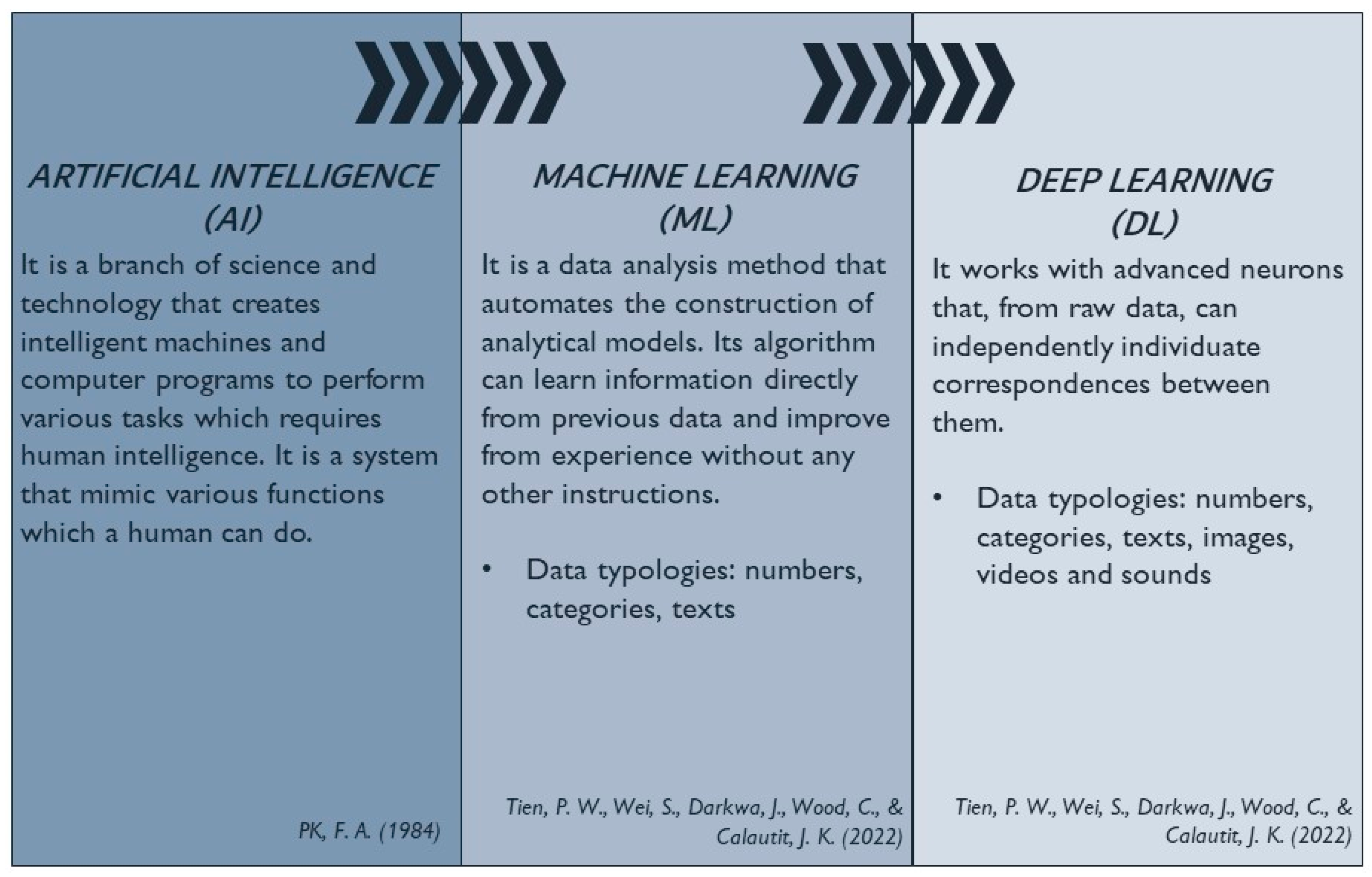
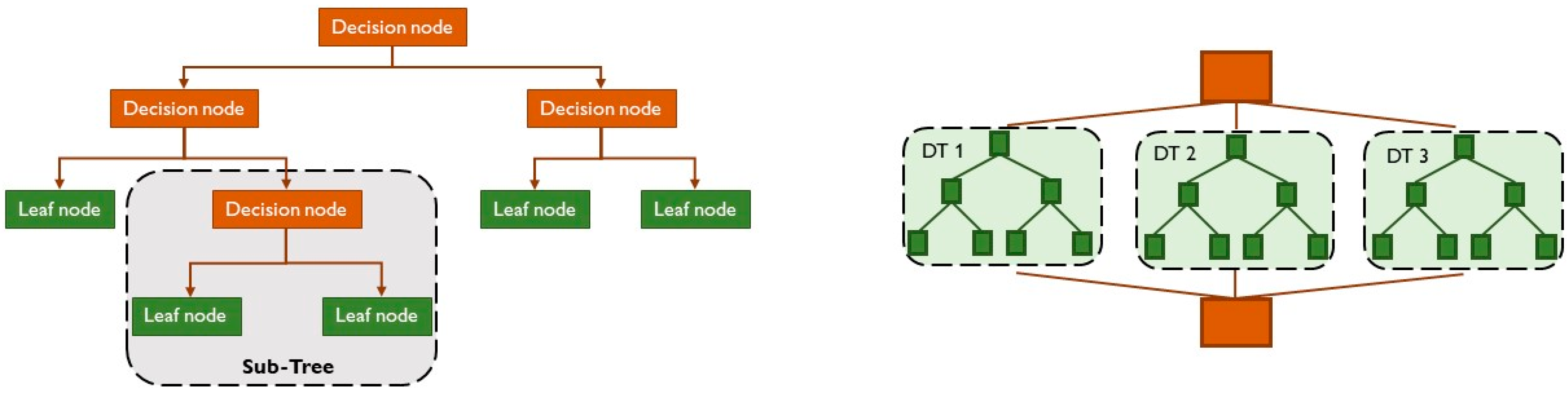
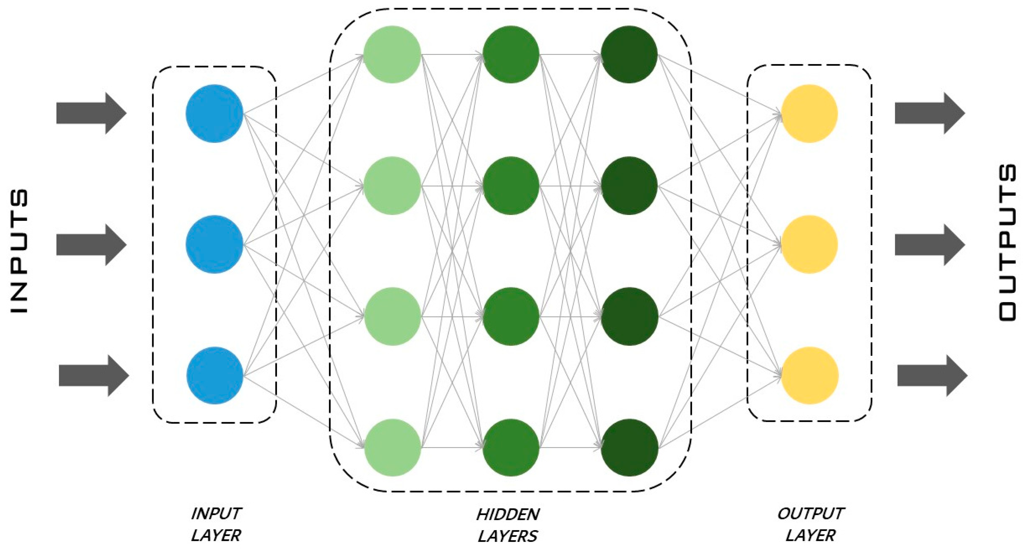
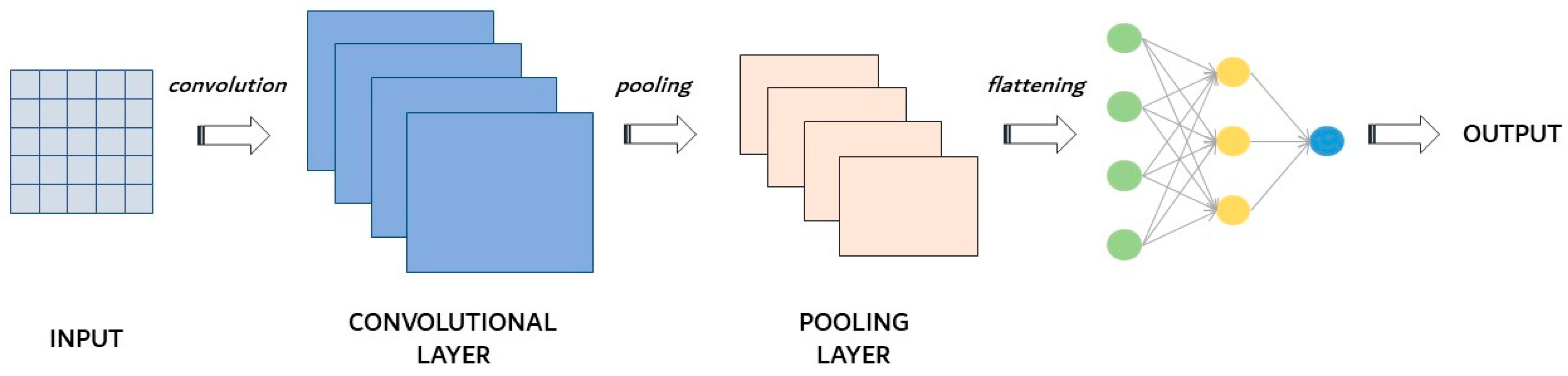
Table 1.
Characterization of recent studies from 2019 to 2023 about machine learning (ML) and deep learning (DL) applied to building energy simulation, optimization and management.
Table 1.
Characterization of recent studies from 2019 to 2023 about machine learning (ML) and deep learning (DL) applied to building energy simulation, optimization and management.
| Authors | Application | ML | DL | ML or DL Technique | Data-Driven (D) or Physically Informed (P) |
|---|---|---|---|---|---|
| Fan et al., (2019) [97] | 1—energy design/optimization | X | RNNs, LSTM, GRUs | D | |
| Xu et al., (2019) [98] | 1 | X | ANNs | D | |
| Pham et al., (2020) [99] | 1 | X | Random forest | D | |
| Zhou et al., (2019) [100] | 1 | X | ANNs, SVMs | D | |
| Liu et al., (2021) [101] | 1 | X | Random forest, ANNs, SVMs | P | |
| Ramos et al., (2022) [102] | 1 | X | ANNs, decision tree | D | |
| Yilmaz et al., (2023) [103] | 1 | X | Naive Bayes, SVMs, random forest | D | |
| Thrampoulidis et al., (2023) [104] | 1 | X | ANNs | P | |
| Xue et al., (2019) [107] | 2—management of energy systems | X | X | LSTM, SVMs, random forest | D |
| Luo et al., (2020) [108] | 2 | X | Genetic algorithm, DNNs | D | |
| Moustakidis et al., (2019) [110] | 2 | X | LSTM | D | |
| Lu et al., (2019) [115] | 2 | X | SVMs, random forest | D | |
| Wei et al., (2020) [111] | 2 | X | CNNs | P | |
| Tien et al., (2021) [112] | 2 | X | CNNs | P | |
| Sha et al., (2021) [114] | 2 | X | X | SVMs, RNNs, CNNs, LSTM | D |
| Somu et al., (2021) [116] | 2 | X | CNNs, LSTM | P | |
| Savadkoohi et al., (2023) [109] | 2 | X | Neural networks | D | |
| Lu et al., (2023) [113] | 2 | X | X | LSTM, CNNs, GRUs, SVMs | D |
| Nabavi et al., (2021) [119] | 3—renewable energy systems | X | LSTM | D | |
| Rana et al., (2022) [120] | 3 | X | X | LSTM, CNNs, random forest | D |
| Mostafa et al., (2022) [121] | 3 | X | X | Random forest, decision trees, CNNs | P |
| Balakumar et al., (2023) [122] | 3 | X | LSTM, GRUs | D | |
| Mirjalili et al., (2023) [123] | 3 | X | X | SVMs, DNNs | P |
| Shahnazari et al., (2019) [127] | 4—fault detection | X | RNNs | P | |
| Taheri et al., (2021) [128] | 4 | X | X | DNNs, random forest | D |
| Ciaburro et al., (2023) [129] | 4 | X | CNNs | P | |
| Copiaco et al., (2023) [130] | 4 | X | X | SVMs, CNNs | p |
| Mustafa et al., (2023) [131] | 4 | X | CNNs, LSTM | P | |
| Albayati et al., (2023) [132] | 4 | X | SVMs | D |
Table 2 summarizes the most commonly used ML/DL methods, with their main applications in the building energy filed.
5. Conclusions
Given the weight of ongoing climate change/global warming and new regulations regarding energy transition, the need to guarantee a “greener” future for the next generations is urgent. This article offers an extensive and comprehensive review of the various machine (ML) and deep learning (DL) techniques applied to the field of building energy simulation, optimization and management.
Modern ML/DL techniques make it easier to create models, i.e., surrogate models, for energy simulations and for optimizing related multi-objective results. Data-driven approaches are more frequent and permit realistic energy prediction trends to be obtained as well as building systems to be controlled/managed.
In this regard, the main aim is to simultaneously address the interplay between energy, the environment and the economy, investigating the optimal solutions for retrofit interventions. Scientific studies are mainly focused on the residential sector, responsible for over one-third of the energy consumption and polluting emissions in the world. Numerous studies have focused on the possibility of optimizing the energy design and/or the choice of retrofit measures to be carried out for predicting the energy consumption of buildings and/or for possible energy savings. To do this, multi-criteria optimization is generally used with cost-optimal solutions to make the building a nearly zero-energy building (nZEB) without neglecting indoor thermal comfort (monitored with Fanger indices). In this regard, artificial neural networks (ANNs) and other ML techniques are widely used, e.g., Bayesian models or support vector machines (SVMs). The control of heating/cooling distribution also involves the use of ANNs or decision trees/random forest models. For the management of renewable sources, DL techniques, e.g., convolutional neural networks (CNNs), recursive neural networks (RNNs), long short-term memory (LSTM) and gated recurrent units (GRUs), are used more frequently, given the large amount of input data and their variability. Malfunction detection can be based on artificial intelligence too, with the use of ML/DL methods, mainly DL. In this sector, intelligent sensors are often used to warn the user about any damage that has occurred so that measures can be taken, safeguarding other subcomponents of the system.
This study shows an increasing diffusion in recent years of ML and DL techniques in the energy field in order to reduce polluting emissions, to deal with climate change and to promote a general energy transition in building stocks. Furthermore, no method appears to be better than another because each one has both its advantages and disadvantages, such as excessively high computational times or overfitting problems. The best approach would be to use one technique or another depending on the case study in question and the desired level of accuracy for the results.
Some limitations of this review article that can be overcome in future include the consideration of the k-nearest, multiple-label gradient boosting, k-means clustering and fuzzy k-means methods.
Funding
This work was supported by the Italian Government MUR PNRR (“Piano Nazionale di Ripresa e Resilienza”).
Conflicts of Interest
The authors declare that they have no known competing financial interests or personal relationships that could have appeared to influence the work reported in this paper.
Nomenclature
| AI | Artificial intelligence |
| ANNs | Artificial neural networks |
| CNNs | Convolutional neural networks |
| DL | Deep learning |
| GRUs | Gated recurrent units |
| LSTM | Long short-term memory |
| ML | Machine learning |
| RNNs | Recursive neural networks |
| SVMs | Support vector machines |
References
- Rocha, P.; Kaut, M.; Siddiqui, A.S. Energy-efficient building retrofits: An assessment of regulatory proposals under uncertainty. Energy 2016, 101, 278–287. [Google Scholar] [CrossRef]
- Khatib, H. IEA world energy outlook 2011—A comment. Energy Policy 2012, 48, 737–743. [Google Scholar] [CrossRef]
- Kottek, M.; Grieser, J.; Beck, C.; Rudolf, B.; Rubel, F. World map of the Köppen-Geiger climate classification updated. Meteorol. Z. 2006, 15, 259–263. [Google Scholar] [CrossRef] [PubMed]
- Lorusso, A.; Maraziti, F. Heating system projects using the degree-days method in livestock buildings. J. Agric. Eng. Res. 1998, 71, 285–290. [Google Scholar] [CrossRef]
- de Llano-Paz, F.; Fernandez, P.M.; Soares, I. Addressing 2030 EU policy framework for energy and climate: Cost, risk and energy security issues. Energy 2016, 115, 1347–1360. [Google Scholar] [CrossRef]
- EU COM 112. A Roadmap for moving to a competitive low carbon economy in 2050. In Communication from the Commission to the European Parliament, the Council, the European Economic and Social Committee and the Committee of the Regions n. 112; European Commission: Brussels, Belgium, 2012.
- EU Commission and Parliament, Directive 2010/31/EU of the EuropeanParliament and of the Council of 19 May 2010 on the energy performance ofbuildings (EPBD Recast). Available online: https://eur-lex.europa.eu/legal-content/EN/TXT/PDF/?uri=CELEX:32010L0031 (accessed on 8 January 2024).
- EU Commission, Commission Delegated Regulation (EU) No 244/2012 of 16 January 2012 Supplementing Directive 2010/31/EU of the EuropeanParliament and of the Council on the Energy Performance of Buildings. Available online: https://eur-lex.europa.eu/LexUriServ/LexUriServ.do?uri=OJ:L:2012:081:0018:0036:en:PDF (accessed on 8 January 2024).
- D.M. (Interministerial Decree) 26 Giugno 2015. Available online: http://www.sviluppoeconomico.gov.it/index.php/it/normativa/decreti-interministeriali/2032966-decreto-interministeriale-26-giugno-2015-applicazione-delle-metodologie-di-calcolo-delle-prestazioni-energetiche-e-definizione-delle-prescrizioni-e-dei-requisiti-minimi-degli-edifici#page_top (accessed on 1 September 2020). (In Italian)
- Cho, H.I.; Cabrera, D.; Patel, M.K. Estimation of energy savings potential through hydraulic balancing of heating systems in buildings. J. Build. Eng. 2020, 28, 101030. [Google Scholar] [CrossRef]
- Nguyen, A.T.; Reiter, S.; Rigo, P. A review on simulation-based optimization methods applied to building performance analysis. Appl. Energy 2014, 113, 1043–1058. [Google Scholar] [CrossRef]
- Aruta, G.; Ascione, F.; Bianco, N.; Mauro, G.M. Sustainability and energy communities: Assessing the potential of building energy retrofit and renewables to lead the local energy transition. Energy 2023, 282, 128377. [Google Scholar] [CrossRef]
- Diakaki, C.; Grigoroudis, E.; Kabelis, N.; Kolokotsa, D.; Kalaitzakis, K.; Stavrakakis, G. A multi-objective decision model for the improvement of energy efficiency in buildings. Energy 2010, 35, 5483–5496. [Google Scholar] [CrossRef]
- Lizana, J.; Molina-Huelva, M.; Chacartegui, R. Multi-criteria assessment for the effective decision management in residential energy retrofitting. Energy Build. 2016, 129, 284–307. [Google Scholar] [CrossRef]
- Fesanghary, M.; Asadi, S.; Geem, Z.W. Design of low-emission and energy-efficient residential buildings using a multi-objective optimization algorithm. Build. Environ. 2012, 49, 245–250. [Google Scholar] [CrossRef]
- Kerdan, I.G.; Raslan, R.; Ruyssevelt, P. An exergy-based multi-objective optimisation model for energy retrofit strategies in non-domestic buildings. Energy 2016, 117, 506–522. [Google Scholar] [CrossRef]
- Harmathy, N.; Magyar, Z.; Folić, R. Multi-criterion optimization of building envelope in the function of indoor illumination quality towards overall energy performance improvement. Energy 2016, 114, 302–317. [Google Scholar] [CrossRef]
- Magnier, L.; Haghighat, F. Multiobjective optimization of building design using TRNSYS simulations, genetic algorithm, and Artificial Neural Network. Build. Environ. 2010, 45, 739–746. [Google Scholar] [CrossRef]
- Li, X.; Malkawi, A. Multi-objective optimization for thermal mass model predictive control in small and medium size commercial buildings under summer weather conditions. Energy 2016, 112, 1194–1206. [Google Scholar] [CrossRef]
- US Department of Energy. Energy Efficiency and Renewable Energy Office, Building Technology Program (2013), EnergyPlus (8.4). Available online: https://energyplus.net/ (accessed on 5 November 2020).
- TRNSYS®, Transient System Simulation Program; University of Wisconsin: Madison, WI, USA, 2000.
- ESP-r. Available online: http://www.esru.strath.ac.uk/Programs/ESP-r.htm (accessed on 5 November 2020).
- IDA-ICE, IDA Indoor Climate and Energy. Available online: http://www.equa.se/ice/intro.html (accessed on 5 November 2020).
- Wang, B.; Xia, X.; Zhang, J. A multi-objective optimization model for the life-cycle cost analysis and retrofitting planning of buildings. Energy Build. 2014, 77, 227–235. [Google Scholar] [CrossRef]
- Suh, W.J.; Park, C.S.; Kim, D.W. Heuristic vs. meta-heuristic optimization for energy performance of a post office building. In Proceedings of the 12th Conference of International Building Performance Simulation Association, Sydney, Australia, 14–16 November 2011; IBPSA: Sydney, Australia, 2011; pp. 704–711. [Google Scholar]
- Ascione, F.; Bianco, N.; De Stasio, C.; Mauro, G.M.; Vanoli, G.P. A new methodology for cost-optimal analysis by means of the multi-objective optimization of building energy performance. Energy Build. 2015, 88, 78–90. [Google Scholar] [CrossRef]
- Hamdy, M.; Hasan, A.; Siren, K. A multi-stage optimization method for cost-optimal and nearly-zero-energy building solutions in line with the EPBD-recast 2010. Energy Build. 2013, 56, 189–203. [Google Scholar] [CrossRef]
- Ferrara, M.; Fabrizio, E.; Virgone, J.; Filippi, M. A simulation-based optimization method for cost-optimal analysis of nearly Zero Energy Buildings. Energy Build. 2014, 84, 442–457. [Google Scholar] [CrossRef]
- Albertin, R.; Prada, A.; Gasparella, A. A novel efficient multi-objective optimization algorithm for expensive building simulation models. Energy Build. 2023, 297, 113433. [Google Scholar] [CrossRef]
- Seçkiner, S.U.; Koç, A. Agent-based simulation and simulation optimization approaches to energy planning under different scenarios: A hospital application case. Comput. Ind. Eng. 2022, 169, 108163. [Google Scholar] [CrossRef]
- Delgarm, N.; Sajadi, B.; Kowsary, F.; Delgarm, S. Multi-objective optimization of the building energy performance: A simulation-based approach by means of particle swarm optimization (PSO). Appl. Energy 2016, 170, 293–303. [Google Scholar] [CrossRef]
- Hamdy, M.; Hasan, A.; Siren, K. Applying a multi-objective optimization approach for design of low-emission cost-effective dwellings. Build. Environ. 2011, 46, 109–123. [Google Scholar] [CrossRef]
- Ascione, F.; Bianco, N.; De Stasio, C.; Mauro, G.M.; Vanoli, G.P. CASA, cost-optimal analysis by multi-objective optimisation and artificial neural networks: A new framework for the robust assessment of cost-optimal energy retrofit, feasible for any building. Energy Build. 2017, 146, 200–219. [Google Scholar] [CrossRef]
- Corgnati, S.P.; Fabrizio, E.; Filippi, M.; Monetti, V. Reference buildings for cost optimal analysis: Method of definition and application. Appl. Energy 2013, 102, 983–993. [Google Scholar] [CrossRef]
- Ashrafian, T.; Yilmaz, A.Z.; Corgnati, S.P.; Moazzen, N. Methodology to define cost-optimal level of architectural measures for energy efficient retrofits of existing detached residential buildings in Turkey. Energy Build. 2016, 120, 58–77. [Google Scholar] [CrossRef]
- Ascione, F.; Cheche, N.; De Masi, R.F.; Minichiello, F.; Vanoli, G.P. Design the refurbishment of historic buildings with the cost-optimal methodology: The case study of a XV century Italian building. Energy Build. 2015, 99, 162–176. [Google Scholar] [CrossRef]
- Pateras, J.; Rana, P.; Ghosh, P. A Taxonomic Survey of Physics-Informed Machine Learning. Appl. Sci. 2023, 13, 6892. [Google Scholar] [CrossRef]
- Montáns, F.J.; Chinesta, F.; Gómez-Bombarelli, R.; Kutz, J.N. Data-driven modeling and learning in science and engineering. Comptes Rendus Mécanique 2019, 347, 845–855. [Google Scholar] [CrossRef]
- Wei, W.; Ramalho, O.; Malingre, L.; Sivanantham, S.; Little, J.C.; Mandin, C. Machine learning and statistical models for predicting indoor air quality. Indoor Air 2019, 29, 704–726. [Google Scholar] [CrossRef] [PubMed]
- Swan, L.G.; Ugursal, V.I. Modeling of end-use energy consumption in the residential sector: A review of modeling techniques. Renew. Sustain. Energy Rev. 2009, 13, 1819–1835. [Google Scholar] [CrossRef]
- Langevin, J.; Reyna, J.L.; Ebrahimigharehbaghi, S.; Sandberg, N.; Fennell, P.; Nägeli, C.; Laverge, J.; Delghust, M.; Mata, É.; Van Hove, M.; et al. Developing a common approach for classifying building stock energy models. Renew. Sustain. Energy Rev. 2020, 133, 110276. [Google Scholar] [CrossRef]
- Bourdeau, M.; Qiangzhai, X.; Nefzaoui, E.; Guo, X.; Chatellier, P. Modeling and forecasting building energy consumption: A review of data-driven techniques. Sustain. Cities Soc. 2019, 48, 101533. [Google Scholar] [CrossRef]
- Mousavi, S.; Marroquín, M.G.V.; Hajiaghaei-Keshteli, M.; Smith, N.R. Data-driven prediction and optimization toward net-zero and positive-energy buildings: A systematic review. Build. Environ. 2023, 242, 110578. [Google Scholar] [CrossRef]
- Fathi, S.; Srinivasan, R.; Fenner, A.; Fathi, S. Machine learning applications in urban building energy performance forecasting: A systematic review. Renew. Sustain. Energy Rev. 2020, 133, 110287. [Google Scholar] [CrossRef]
- Tien, P.W.; Wei, S.; Darkwa, J.; Wood, C.; Calautit, J.K. Machine learning and deep learning methods for enhancing building energy efficiency and indoor environmental quality—A review. Energy AI 2022, 10, 100198. [Google Scholar] [CrossRef]
- Pan, Y.; Zhu, M.; Lv, Y.; Yang, Y.; Liang, Y.; Yin, R.; Yang, Y.; Jia, X.; Wang, X.; Zeng, F.; et al. Building energy simulation and its application for building performance optimization: A review of methods, tools, and case studies. Adv. Appl. Energy 2023, 10, 100135. [Google Scholar] [CrossRef]
- PK, F.A. What is artificial intelligence? In Learning Outcomes of Classroom Research; L’ Ordine Nuovo Publication: Turin, Italy, 1984; p. 65. [Google Scholar]
- Boeschoten, S.; Catal, C.; Tekinerdogan, B.; Lommen, A.; Blokland, M. The automation of the development of classification models and improvement of model quality using feature engineering techniques. Expert Syst. Appl. 2023, 213, 118912. [Google Scholar] [CrossRef]
- Nasteski, V. An overview of the supervised machine learning methods. Horizons. B 2017, 4, 51–62. [Google Scholar] [CrossRef]
- Geysen, D.; De Somer, O.; Johansson, C.; Brage, J.; Vanhoudt, D. Operational thermal load forecasting in district heating networks using machine learning and expert advice. Energy Build. 2018, 162, 144–153. [Google Scholar] [CrossRef]
- Somvanshi, M.; Chavan, P.; Tambade, S.; Shinde, S.V. A review of machine learning techniques using decision tree and support vector machine. In Proceedings of the 2016 International Conference on Computing Communication Control and Automation (ICCUBEA), Pune, India, 12–13 August 2016; pp. 1–7. [Google Scholar]
- Ryu, S.H.; Moon, H.J. Development of an occupancy prediction model using indoor environmental data based on machine learning techniques. Build. Environ. 2016, 107, 1–9. [Google Scholar] [CrossRef]
- Daniya, T.; Geetha, M.; Kumar, K.S. Classification and regression trees with gini index. Adv. Math. Sci. J. 2020, 9, 8237–8247. [Google Scholar] [CrossRef]
- Rodriguez-Galiano, V.; Sanchez-Castillo, M.; Chica-Olmo, M.; Chica-Rivas, M.J. Machine learning predictive models for mineral prospectivity: An evaluation of neural networks, random forest, regression trees and support vector machines. Ore Geol. Rev. 2015, 71, 804–818. [Google Scholar] [CrossRef]
- Chou, J.S.; Bui, D.K. Modeling heating and cooling loads by artificial intelligence for energy-efficient building design. Energy Build. 2014, 82, 437–446. [Google Scholar] [CrossRef]
- Sapnken, F.E.; Hamed, M.M.; Soldo, B.; Tamba, J.G. Modeling energy-efficient building loads using machine-learning algorithms for the design phase. Energy Build. 2023, 283, 112807. [Google Scholar] [CrossRef]
- Cai, W.; Wei, R.; Xu, L.; Ding, X. A method for modelling greenhouse temperature using gradient boost decision tree. Inf. Process. Agric. 2022, 9, 343–354. [Google Scholar] [CrossRef]
- Chen, Y.T.; Piedad, E., Jr.; Kuo, C.C. Energy consumption load forecasting using a level-based random forest classifier. Symmetry 2019, 11, 956. [Google Scholar] [CrossRef]
- Vishwakarma, M.; Kesswani, N. A new two-phase intrusion detection system with Naïve Bayes machine learning for data classification and elliptic envelop method for anomaly detection. Decis. Anal. J. 2023, 7, 100233. [Google Scholar] [CrossRef]
- Bassamzadeh, N.; Ghanem, R. Multiscale stochastic prediction of electricity demand in smart grids using Bayesian networks. Appl. Energy 2017, 193, 369–380. [Google Scholar] [CrossRef]
- Hosamo, H.H.; Nielsen, H.K.; Kraniotis, D.; Svennevig, P.R.; Svidt, K. Improving building occupant comfort through a digital twin approach: A Bayesian network model and predictive maintenance method. Energy Build. 2023, 288, 112992. [Google Scholar] [CrossRef]
- Vapnik, V. The Nature of Statistical Learning Theory; Springer Science & Business Media: Berlin/Heidelberg, Germany, 1999. [Google Scholar]
- Dong, B.; Cao, C.; Lee, S.E. Applying support vector machines to predict building energy consumption in tropical region. Energy Build. 2005, 37, 545–553. [Google Scholar] [CrossRef]
- Ahmad, M.W.; Reynolds, J.; Rezgui, Y. Predictive modelling for solar thermal energy systems: A comparison of support vector regression, random forest, extra trees and regression trees. J. Clean. Prod. 2018, 203, 810–821. [Google Scholar] [CrossRef]
- Kapp, S.; Choi, J.K.; Hong, T. Predicting industrial building energy consumption with statistical and machine-learning models informed by physical system parameters. Renew. Sustain. Energy Rev. 2023, 172, 113045. [Google Scholar] [CrossRef]
- Kim, J.B.; Kim, S.E.; Aman, J.A. An urban building energy simulation method integrating parametric BIM and machine learning. In Proceedings of the Human-Centric, 27th International Conference of the Association for Computer-Aided Architectural Design Research in Asia (CAADRIA), Sydney, Australia, 28 September 2021–26 January 2022; pp. 18–24. [Google Scholar]
- Krige, D.G. A Statistical Approach to Some Mine Valuation and Allied Problems on the Witwatersrand: By DG Krige. Ph.D. Thesis, University of the Witwatersrand, Johannesburg, South Africa, 1951. [Google Scholar]
- Matheron, G. The selectivity of the distributions and “the second principle of geostatistics”. In Geostatistics for Natural Resources Characterization. Part 1; Springer: Dordrecht, The Netherlands, 1984; pp. 421–433. [Google Scholar] [CrossRef]
- Martin, J.D.; Simpson, T.W. Use of kriging models to approximate deterministic computer models. AIAA J. 2005, 43, 853–863. [Google Scholar] [CrossRef]
- Cressie, N. Statistics for Spatial Data; John Wiley & Sons: Hoboken, NJ, USA, 2015. [Google Scholar]
- Kleijnen, J.P. Kriging metamodeling in simulation: A review. Eur. J. Oper. Res. 2009, 192, 707–716. [Google Scholar] [CrossRef]
- Eguía, P.; Granada, E.; Alonso, J.M.; Arce, E.; Saavedra, A. Weather datasets generated using kriging techniques to calibrate building thermal simulations with TRNSYS. J. Build. Eng. 2016, 7, 78–91. [Google Scholar] [CrossRef]
- Hopfe, C.J.; Emmerich, M.T.; Marijt, R.; Hensen, J. Robust multi-criteria design optimisation in building design. Proc. Build. Simul. Optim. 2012, 118–125. Available online: https://publications.ibpsa.org/conference/paper/?id=bso2012_1A3 (accessed on 8 January 2024).
- Tresidder, E.; Zhang, Y.; Forrester, A.I. Acceleration of building design optimisation through the use of kriging surrogate models. Proc. Build. Simul. Optim. 2012, 2012, 1–8. [Google Scholar]
- Almutairi, K.; Aungkulanon, P.; Algarni, S.; Alqahtani, T.; Keshuov, S.A. Solar irradiance and efficient use of energy: Residential construction toward net-zero energy building. Sustain. Energy Technol. Assess. 2022, 53, 102550. [Google Scholar] [CrossRef]
- Küçüktopcu, E.; Cemek, B.; Simsek, H. Application of Spatial Analysis to Determine the Effect of Insulation Thickness on Energy Efficiency and Cost Savings for Cold Storage. Processes 2022, 10, 2393. [Google Scholar] [CrossRef]
- Naji, S.; Keivani, A.; Shamshirband, S.; Alengaram, U.J.; Jumaat, M.Z.; Mansor, Z.; Lee, M. Estimating building energy consumption using extreme learning machine method. Energy 2016, 97, 506–516. [Google Scholar] [CrossRef]
- Uzair, M.; Jamil, N. Effects of hidden layers on the efficiency of neural networks. In Proceedings of the 2020 IEEE 23rd International Multitopic Conference (INMIC), Bahawalpur, Pakistan, 5–7 November 2020; pp. 1–6. [Google Scholar]
- Li, Y.F.; Ng, S.H.; Xie, M.; Goh, T.N. A systematic comparison of metamodeling techniques for simulation optimization in decision support systems. Appl. Soft Comput. 2010, 10, 1257–1273. [Google Scholar] [CrossRef]
- Ascione, F.; Bianco, N.; De Stasio, C.; Mauro, G.M.; Vanoli, G.P. Artificial neural networks to predict energy performance and retrofit scenarios for any member of a building category: A novel approach. Energy 2017, 118, 999–1017. [Google Scholar] [CrossRef]
- Fanger, P.O. Thermal comfort. Analysis and applications in environmental engineering. In Thermal Comfort. Analysis and Applications in Environmental Engineering; McGraw Hill: New York, NY, USA, 1970. [Google Scholar]
- Asadi, E.; Da Silva, M.G.; Antunes, C.H.; Dias, L.; Glicksman, L. Multi-objective optimization for building retrofit: A model using genetic algorithm and artificial neural network and an application. Energy Build. 2014, 81, 444–456. [Google Scholar] [CrossRef]
- Melo, A.P.; Cóstola, D.; Lamberts, R.; Hensen, J.L.M. Development of surrogate models using artificial neural network for building shell energy labelling. Energy Policy 2014, 69, 457–466. [Google Scholar] [CrossRef]
- Pérez-Gomariz, M.; López-Gómez, A.; Cerdán-Cartagena, F. Artificial neural networks as artificial intelligence technique for energy saving in refrigeration systems—A review. Clean Technol. 2023, 5, 116–136. [Google Scholar] [CrossRef]
- Chen, X.; Cao, B.; Pouramini, S. Energy cost and consumption reduction of an office building by Chaotic Satin Bowerbird Optimization Algorithm with model predictive control and artificial neural network: A case study. Energy 2023, 270, 126874. [Google Scholar] [CrossRef]
- Zhang, H.; Feng, H.; Hewage, K.; Arashpour, M. Artificial neural network for predicting building energy performance: A surrogate energy retrofits decision support framework. Buildings 2022, 12, 829. [Google Scholar] [CrossRef]
- Singaravel, S.; Suykens, J.; Geyer, P. Deep-learning neural-network architectures and methods: Using component-based models in building-design energy prediction. Adv. Eng. Inform. 2018, 38, 81–90. [Google Scholar] [CrossRef]
- Wang, H.; Lei, Z.; Zhang, X.; Zhou, B.; Peng, J. A review of deep learning for renewable energy forecasting. Energy Convers. Manag. 2019, 198, 111799. [Google Scholar] [CrossRef]
- Amarasinghe, K.; Marino, D.L.; Manic, M. Deep neural networks for energy load forecasting. In Proceedings of the 2017 IEEE 26th International Symposium on Industrial Electronics (ISIE), Edinburgh, UK, 19–21 June 2017; pp. 1483–1488. [Google Scholar]
- Khan, Z.A.; Hussain, T.; Haq, I.U.; Ullah, F.U.M.; Baik, S.W. Towards efficient and effective renewable energy prediction via deep learning. Energy Rep. 2022, 8, 10230–10243. [Google Scholar] [CrossRef]
- Kim, T.Y.; Cho, S.B. Predicting residential energy consumption using CNN-LSTM neural networks. Energy 2019, 182, 72–81. [Google Scholar] [CrossRef]
- Jebli, I.; Belouadha, F.Z.; Kabbaj, M.I.; Tilioua, A. Deep learning based models for solar energy prediction. Advances in Science. Technol. Eng. Syst. J. 2021, 6, 349–355. [Google Scholar]
- Karijadi, I.; Chou, S.Y. A hybrid RF-LSTM based on CEEMDAN for improving the accuracy of building energy consumption prediction. Energy Build. 2022, 259, 111908. [Google Scholar] [CrossRef]
- Peng, L.; Wang, L.; Xia, D.; Gao, Q. Effective energy consumption forecasting using empirical wavelet transform and long short-term memory. Energy 2022, 238, 121756. [Google Scholar] [CrossRef]
- Abid, F.; Alam, M.; Alamri, F.S.; Siddique, I. Multi-directional gated recurrent unit and convolutional neural network for load and energy forecasting: A novel hybridization. AIMS Math. 2023, 8, 19993–20017. [Google Scholar] [CrossRef]
- Jiao, Y.; Tan, Z.; Zhang, D.; Zheng, Q.P. Short-term building energy consumption prediction strategy based on modal decomposition and reconstruction algorithm. Energy Build. 2023, 290, 113074. [Google Scholar] [CrossRef]
- Fan, C.; Wang, J.; Gang, W.; Li, S. Assessment of deep recurrent neural network-based strategies for short-term building energy predictions. Appl. Energy 2019, 236, 700–710. [Google Scholar] [CrossRef]
- Xu, X.; Wang, W.; Hong, T.; Chen, J. Incorporating machine learning with building network analysis to predict multi-building energy use. Energy Build. 2019, 186, 80–97. [Google Scholar] [CrossRef]
- Pham, A.D.; Ngo, N.T.; Truong, T.T.H.; Huynh, N.T.; Truong, N.S. Predicting energy consumption in multiple buildings using machine learning for improving energy efficiency and sustainability. J. Clean. Prod. 2020, 260, 121082. [Google Scholar] [CrossRef]
- Zhou, Y.; Zheng, S. Machine-learning based hybrid demand-side controller for high-rise office buildings with high energy flexibilities. Appl. Energy 2020, 262, 114416. [Google Scholar] [CrossRef]
- Liu, Y.; Chen, H.; Zhang, L.; Feng, Z. Enhancing building energy efficiency using a random forest model: A hybrid prediction approach. Energy Rep. 2021, 7, 5003–5012. [Google Scholar] [CrossRef]
- Ramos, D.; Faria, P.; Morais, A.; Vale, Z. Using decision tree to select forecasting algorithms in distinct electricity consumption context of an office building. Energy Rep. 2022, 8, 417–422. [Google Scholar] [CrossRef]
- Yılmaz, D.; Tanyer, A.M.; Toker, İ.D. A data-driven energy performance gap prediction model using machine learning. Renew. Sustain. Energy Rev. 2023, 181, 113318. [Google Scholar] [CrossRef]
- Thrampoulidis, E.; Hug, G.; Orehounig, K. Approximating optimal building retrofit solutions for large-scale retrofit analysis. Appl. Energy 2023, 333, 120566. [Google Scholar] [CrossRef]
- Sajjadi, S.; Shamshirband, S.; Alizamir, M.; Yee, L.; Mansor, Z.; Manaf, A.A.; Altameem, T.A.; Mostafaeipour, A. Extreme learning machine for prediction of heat load in district heating systems. Energy Build. 2016, 122, 222–227. [Google Scholar] [CrossRef]
- Saloux, E.; Candanedo, J.A. Forecasting district heating demand using machine learning algorithms. Energy Procedia 2018, 149, 59–68. [Google Scholar] [CrossRef]
- Xue, G.; Pan, Y.; Lin, T.; Song, J.; Qi, C.; Wang, Z. District heating load prediction algorithm based on feature fusion LSTM model. Energies 2019, 12, 2122. [Google Scholar] [CrossRef]
- Luo, X.J.; Oyedele, L.O.; Ajayi, A.O.; Akinade, O.O.; Owolabi, H.A.; Ahmed, A. Feature extraction and genetic algorithm enhanced adaptive deep neural network for energy consumption prediction in buildings. Renenable Sustain. Energy Rev. 2020, 131, 109980. [Google Scholar] [CrossRef]
- Savadkoohi, M.; Macarulla, M.; Casals, M. Facilitating the implementation of neural network-based predictive control to optimize building heating operation. Energy 2023, 263, 125703. [Google Scholar] [CrossRef]
- Moustakidis, S.; Meintanis, I.; Karkanias, N.; Halikias, G.; Saoutieff, E.; Gasnier, P.; Ojer-Aranguren, J.; Anagnostis, A.; Marciniak, B.; Rodot, I.; et al. Innovative technologies for district heating and cooling: InDeal Project. Proceedings 2019, 5, 1. [Google Scholar]
- Wei, S.; Tien, P.W.; Calautit, J.K.; Wu, Y.; Boukhanouf, R. Vision-based detection and prediction of equipment heat gains in commercial office buildings using a deep learning method. Appl. Energy 2020, 277, 115506. [Google Scholar] [CrossRef]
- Tien, P.W.; Wei, S.; Calautit, J.K.; Darkwa, J.; Wood, C. Occupancy heat gain detection and prediction using deep learning approach for reducing building energy demand. J. Sustain. Dev. Energy Water Environ. Syst. 2021, 9, 1–31. [Google Scholar] [CrossRef]
- Lu, C.; Gu, J.; Lu, W. An improved attention-based deep learning approach for robust cooling load prediction: Public building cases under diverse occupancy schedules. Sustain. Cities Soc. 2023, 96, 104679. [Google Scholar] [CrossRef]
- Sha, H.; Moujahed, M.; Qi, D. Machine learning-based cooling load prediction and optimal control for mechanical ventilative cooling in high-rise buildings. Energy Build. 2021, 242, 110980. [Google Scholar] [CrossRef]
- Lu, S.; Wang, W.; Lin, C.; Hameen, E.C. Data-driven simulation of a thermal comfort-based temperature set-point control with ASHRAE RP884. Build. Environ. 2019, 156, 137–146. [Google Scholar] [CrossRef]
- Somu, N.; Sriram, A.; Kowli, A.; Ramamritham, K. A hybrid deep transfer learning strategy for thermal comfort prediction in buildings. Build. Environ. 2021, 204, 108133. [Google Scholar] [CrossRef]
- Yaïci, W.; Entchev, E. Performance prediction of a solar thermal energy system using artificial neural networks. Appl. Therm. Eng. 2014, 73, 1348–1359. [Google Scholar] [CrossRef]
- Mocanu, E.; Nguyen, P.H.; Gibescu, M.; Kling, W.L. Deep learning for estimating building energy consumption. Sustain. Energy Grids Netw. 2016, 6, 91–99. [Google Scholar] [CrossRef]
- Nabavi, S.A.; Motlagh, N.H.; Zaidan, M.A.; Aslani, A.; Zakeri, B. Deep learning in energy modeling: Application in smart buildings with distributed energy generation. IEEE Access 2021, 9, 125439–125461. [Google Scholar] [CrossRef]
- Rana, M.; Sethuvenkatraman, S.; Heidari, R.; Hands, S. Solar thermal generation forecast via deep learning and application to buildings cooling system control. Renew. Energy 2022, 196, 694–706. [Google Scholar] [CrossRef]
- Mostafa, N.; Ramadan, H.S.M.; Elfarouk, O. Renewable energy management in smart grids by using big data analytics and machine learning. Mach. Learn. Appl. 2022, 9, 100363. [Google Scholar] [CrossRef]
- Balakumar, P.; Vinopraba, T.; Chandrasekaran, K. Deep learning based real time Demand Side Management controller for smart building integrated with renewable energy and Energy Storage System. J. Energy Storage 2023, 58, 106412. [Google Scholar] [CrossRef]
- Mirjalili, M.A.; Aslani, A.; Zahedi, R.; Soleimani, M. A comparative study of machine learning and deep learning methods for energy balance prediction in a hybrid building-renewable energy system. Sustain. Energy Res. 2023, 10, 8. [Google Scholar] [CrossRef]
- Nelson, W.; Culp, C. Machine Learning Methods for Automated Fault Detection and Diagnostics in Building Systems—A Review. Energies 2022, 15, 5534. [Google Scholar] [CrossRef]
- Zhao, Y.; Li, T.; Zhang, X.; Zhang, C. Artificial intelligence-based fault detection and diagnosis methods for building energy systems: Advantages, challenges and the future. Renew. Sustain. Energy Rev. 2019, 109, 85–101. [Google Scholar] [CrossRef]
- Liang, J.; Du, R. Model-based fault detection and diagnosis of HVAC systems using support vector machine method. Int. J. Refrig. 2007, 30, 1104–1114. [Google Scholar] [CrossRef]
- Shahnazari, H.; Mhaskar, P.; House, J.M.; Salsbury, T.I. Modeling and fault diagnosis design for HVAC systems using recurrent neural networks. Comput. Chem. Eng. 2019, 126, 189–203. [Google Scholar] [CrossRef]
- Taheri, S.; Ahmadi, A.; Mohammadi-Ivatloo, B.; Asadi, S. Fault detection diagnostic for HVAC systems via deep learning algorithms. Energy Build. 2021, 250, 111275. [Google Scholar] [CrossRef]
- Ciaburro, G.; Padmanabhan, S.; Maleh, Y.; Puyana-Romero, V. Fan Fault Diagnosis Using Acoustic Emission and Deep Learning Methods. Informatics 2023, 10, 24. [Google Scholar] [CrossRef]
- Copiaco, A.; Himeur, Y.; Amira, A.; Mansoor, W.; Fadli, F.; Atalla, S.; Sohail, S.S. An innovative deep anomaly detection of building energy consumption using energy time-series images. Eng. Appl. Artif. Intell. 2023, 119, 105775. [Google Scholar] [CrossRef]
- Mustafa, Z.; Awad, A.S.; Azzouz, M.; Azab, A. Fault identification for photovoltaic systems using a multi-output deep learning approach. Expert Syst. Appl. 2023, 211, 118551. [Google Scholar] [CrossRef]
- Albayati, M.G.; Faraj, J.; Thompson, A.; Patil, P.; Gorthala, R.; Rajasekaran, S. Semi-supervised machine learning for fault detection and diagnosis of a rooftop unit. Big Data Min. Anal. 2023, 6, 170–184. [Google Scholar] [CrossRef]
Figure 1.
Differences between machine and deep learning. PK, F.A. (1984) [47]. Tien, P. W., Wei, S., Darkwa, J., Wood, C., & Calautit, J. K. (2022) [45].

Figure 2.
Machine learning methods.

Figure 3.
Supervised learning: classification (left) and regression (right).

Figure 4.
Unsupervised learning: clustering (left) and association (right).

Figure 5.
Reinforcement learning.

Figure 6.
Decision trees (DTs) (left) and random forest (right).

Figure 7.
SVM hyperplane: (a) feature space scheme; (b) noise example; (c) Kernel function.

Figure 8.
Scheme of an artificial neural network.

Figure 9.
Convolutional neural network scheme.

Figure 10.
Recursive neural network scheme.

Figure 11.
Long short-term memory network scheme.

Table 2.
ML/DL methods investigated in this paper and their main applications in the building energy field.
Table 2.
ML/DL methods investigated in this paper and their main applications in the building energy field.
| Technique | ML | DL | Characterization | Applications |
|---|---|---|---|---|
| Decision trees | X | Can handle heterogeneous data; simple to use; overfitting problems | Prediction and control | |
| Random forest | X | Accurate; less overfitting problems; computationally expensive | Prediction, control and fault detection | |
| Naive Bayes | X | Simple to use; limited applicability | Control | |
| SVMs | X | Can handle high-dimensional and non-linear data; computationally expensive; careful choice of the hyperparameters | Prediction, control and fault detection | |
| ANNs | X | X | Can handle big dataset and non-linear data correlations; can solve complex problems; require large training dataset | Prediction and control |
| CNNs | X | Can learn features automatically; useful for image classification and recognition; require large training dataset; computationally expensive | Prediction, control and fault detection | |
| RNNs | X | Can handle sequential data and learn long-term dependencies; overfitting and vanishing gradient problems | Prediction, control and fault detection | |
| LSTM | X | Can learn long-term dependencies; possible vanishing gradient problems | Prediction, control and fault detection | |
| GRUs | X | Fast training; can handle high-dimensional data; no vanishing gradient problems | Prediction and control |
Disclaimer/Publisher’s Note: The statements, opinions and data contained in all publications are solely those of the individual author(s) and contributor(s) and not of MDPI and/or the editor(s). MDPI and/or the editor(s) disclaim responsibility for any injury to people or property resulting from any ideas, methods, instructions or products referred to in the content. |
© 2024 by the authors. Licensee MDPI, Basel, Switzerland. This article is an open access article distributed under the terms and conditions of the Creative Commons Attribution (CC BY) license (https://creativecommons.org/licenses/by/4.0/).
Share and Cite
MDPI and ACS Style
Villano, F.; Mauro, G.M.; Pedace, A. A Review on Machine/Deep Learning Techniques Applied to Building Energy Simulation, Optimization and Management. Thermo 2024, 4, 100-139. https://0-doi-org.brum.beds.ac.uk/10.3390/thermo4010008
AMA Style
Villano F, Mauro GM, Pedace A. A Review on Machine/Deep Learning Techniques Applied to Building Energy Simulation, Optimization and Management. Thermo. 2024; 4(1):100-139. https://0-doi-org.brum.beds.ac.uk/10.3390/thermo4010008
Chicago/Turabian StyleVillano, Francesca, Gerardo Maria Mauro, and Alessia Pedace. 2024. "A Review on Machine/Deep Learning Techniques Applied to Building Energy Simulation, Optimization and Management" Thermo 4, no. 1: 100-139. https://0-doi-org.brum.beds.ac.uk/10.3390/thermo4010008