
Young vs. Old Population: Does Urban Environment of Skyscrapers Create Different Obesity Prevalence?


1
Sir Harry Solomon School of Economics and Management, Western Galilee College, Derech Hamichlalot, Acre 2412101, Israel
2
Department of Mathematics, Bar Ilan University, 1 Max and Anna Web Street, Ramat Gan 5290002, Israel
3
School of Real Estate, Netanya Academic College, 1 University Street, Netanya 4223587, Israel
4
The Ruth and Bruce Rapoport Faculty of Medicine, Technion—Israel Institute of Technology, 1 Efron Street, Haifa 3525422, Israel
5
Department of Dermatology, Emek Medical Center, 21 Yitshak Rabin Boulevard, Afula 1834111, Israel
*
Author to whom correspondence should be addressed.
BioMed 2023, 3(4), 440-459; https://0-doi-org.brum.beds.ac.uk/10.3390/biomed3040036
Submission received: 28 June 2023
/
Revised: 1 October 2023
/
Accepted: 7 October 2023
/
Published: 24 October 2023
Abstract
:This study investigates the impact of more densely populated urban environments proxied by the number of skyscrapers on the obesity prevalence among young vs. old populations at a US statewide level. Obesity is a global pandemic, as well as a major risk factor for a long series of health problems and increased mortality rates. We employ a quadratic model, which relaxes the a priori assumption of the monotonic rise or drop in obesity prevalence with the number of skyscrapers. The outcomes demonstrated a U-shaped curve and a sharper decrease (increase) in the projected obesity prevalence with the number of skyscrapers in the range of 0–147 (147–270) skyscrapers for the old population age cohorts above 65 years old. One possible explanation is the different motivation for physical activity among dissimilar age cohorts. While younger people are focused on maintaining a slim body shape, older people identify with the importance of sports. The public policy outcome of our study is the need to implement different recommendations in dissimilar urban environments based on age cohort stratification. Given that skyscrapers are the manifestation of wealth economics and present the typical characteristics of modern cities, which, in turn, are the future of economic development and productivity, these recommendations might prove to be important.
1. Introduction
1.1. Background
Skyscrapers are the manifestation of wealth economics and present the typical characteristics of modern cities, which, in turn, are the future of economic development and productivity [1,2,3]. High population densities are associated with high-rise buildings and expensive land prices [4,5].
The relationship between the number of skyscrapers and dense urban environments is well established in the urban economic literature and dates back to Wiliam Alonso [6,7] and Richard F. Muth [8]. They laid out a basic theoretical model, where location decisions were made via bidding on land, wherein the highest bidder outbid other potential users, firms, or households [9]. Alonso [6] investigated the research question as to why four-fifths of privately developed land in typical American cities is occupied by residential housing, while implicitly the other one fifth is occupied by office buildings [10]. A more direct statement was made in the introduction of Muth [8], who described car travel in a typical American city where the landscape is modified from high-rise buildings to single family units. This gave rise to the development of the urban monocentric model, where all employment is located at the city center. A formal derivation is given in [11] (pp. 425–431). Given that land resources in the city center (suburbs) are rather expensive and scarce (cheap and abundant), it makes economic sense to save land (capital) and construct high-rise buildings (detached single-family housing units). A quantitative measure for the responsiveness of the developer to modifications in land prices is the land-to-structure elasticity of substitution [12].
Cities also influence important aspects of health [13,14,15]. This is manifested, inter alia, by obesity prevalence. Obesity is a global pandemic, as well as a major risk factor for a long series of health problems and increased mortality rates. According to the World Health Organization [16], obesity is defined as a BMI ≥ 30 (). Diseases associated with obesity include musculoskeletal disorders (particularly osteoarthritis—a highly disabling degenerative disease of the joints); cardiovascular diseases (mainly heart disease and stroke—which were the leading causes of mortality in 2012); and diabetes [16]. The built environment can contribute to health outcomes via two main pathways: (1) biological responses to environmental exposures, such as air pollution, and (2) obesogenic behaviors such as physical activity and diet. In that context, Zaccardi et al. [17] suggested that, with the exception of smoking, slow walkers with an otherwise healthy lifestyle have a higher mortality risk than brisk walkers. The latter pathway of obesogenic behaviors is related to the ways in which land use and transportation planning can support healthy behaviors [18].
The relationships between walkability, obesity, and dense urban environments is supported by a long list of empirical studies [18,19,20,21]. In 2005, the relationship between the levels of physical activity and urban environments was identified as a relatively new field of study [19]. Physical inactivity is considered to be responsible for increased mortality rates of up to 20–30% [16,20,22]. A decrease in physical activity levels over time might be an outcome of the urban sprawl phenomenon, namely, more occupied residential land following population growth ([5] (pp. 181–186)). This, in turn, prolongs travel distances and makes the private vehicle the most convenient and practical means of transportation. In urban planning, compact development (i.e., the dense construction mode) is associated with a reduction in automobile dependence [21]. Indeed, in 2005—during which only 45% of the US adult population declared to engaging in at least 30 min daily vigorous walking—this was considered to be mild physical activity ([19] p. 2).
Urban environments combine disadvantages and advantages in terms of obesity, nutrition, and physical activity. On the one hand, crowded cities, characterized by high population densities, may discourage physical activity and provide more opportunities for the increased consumption of ill-nutritional food during the nights and concurrent sleep deprivation [23,24,25]. Chen and Zhou [26] found that the densities of four-way intersections and more than five-way intersections and land use mixture were positively correlated with pedestrian crash frequency and risk in Seattle, Washington. Given studies that found no correlation between specific built environments and walking, Feuillet et al. [27] suggested that more subtle analysis is required. Nigg et al. [28] demonstrated that for more densely populated and crowded regions in Germany, less positive physical activity changes were observed during the first COVID-19 lockdown in April 2020 among children. Finally, referring to the older population in Japan, Hino and Asami [29] found that a high walkability neighborhood adversely affected step counts, whereas proximity to large parks had a positive effect during the COVID19 state-of-emergency period.
On the other hand, such environments may promote walkability by including bicycle and running tracks, green spaces and parks, gyms, stairways, and mixed uses of land. Few articles emphasize the argument that some built environment characteristics encourage people to increase their walking distances [30,31,32]. Based on a longitudinal study of Canadians, the exposure to walkable neighborhoods in urban areas increased utilitarian walking [33].
1.2. The Current Study: Descriptions and Contributions
In this manuscript, we examine whether the urban environments of skyscrapers create different patterns of obesity prevalence among the young vs. old population [The definition of young (old) age cohorts is 18–25 years (65 + years)]. Obesity is closely related to genetic and environmental factors [34,35], as well as nutrition and physical activity [36,37]. Sallis et al. [35] suggest that the design of urban environments has the potential to contribute substantially to physical activity. The motivation for physical activity is different among the dissimilar age cohorts. While the concerns of younger people are focused on maintaining a slim body shape, older people identify with the importance of sports and physical activity in removing aging effects and providing a social support network [38]. These components might explain the outcomes obtained in this study referring to young–old differences in obesity prevalence.
The motivation for physical activity (PA) is a major topic in psychology, with at least 32 theories trying to explain either the motivation or the lack of it. According to the self-determination theory (SDT), people are motivated by three basic needs, namely, competence, autonomy, and social relatedness [39]. While intrinsic motivation comes from within, extrinsic motivation arises from outside. When an individual is intrinsically motivated, he or she engages in an activity solely based on inner satisfaction and enjoyment. The literature contains a discussion on the intrinsic motivation for PA of both adolescents [40,41,42] and elderly populations [43,44,45].
Referring to the young populations, Kalajas-Tilga et al. [41] demonstrated that SDT-based models explained the medium-to-vigorous physical activity (MVPA) of adolescents. The authors stress the special focus required to increase intrinsic motivation toward physical education. Given that teachers’ behaviors are a key factor that influences students’ motivation, Ahmadi et al. [42], proposed a classification system of traits based on a forum of panel experts. Ahmed et al. [40], provided continuing support for the investigation conducted by Allender et al. [38]. In their review, the authors highlighted a major volume of research indicating that during the period of adolescence, individuals are often competitive and demonstrate a challenging attitude with respect to tasks; hence, they have a greater tendency to maintain a positive body image as a form of competition with their peers. This is perhaps the reason why in Ahmed et al. [40], fitness and health received such a high score among girls.
A few studies followed that of Allender et al. [38] (e.g., [40,46]). Firestone et al. [46] investigated adult New Yorkers during 2010–2011. The authors found overall that 70.6% of adult New Yorkers reported having physically active friends. Having active friends was associated with increased leisure time for physical activity by a factor of two times more activity (56 min/week) for men and two and a half times more activity (35 min/week) for women. Physically active males and females who usually engaged in leisure time activities as a part of a group reported 1.4 times more activity than those who exercised alone.
Ahmed et al. [40], provided continuing support for the investigation conducted by Allender et al. [38]. In their review, the authors highlighted a major volume of research indicating that during the period of adolescence, individuals are often competitive and demonstrate a challenging attitude with respect to tasks; hence, they have a greater tendency to maintain a positive body image as a form of competition with their peers. This is perhaps the reason why in Ahmed et al. [40], fitness and health received such a high score among girls.
The data employed in this study referred to obesity prevalence at a US statewide level in 2011–2020 obtained from the Center for Disease Control and Prevention [47]. The definition of skyscrapers employed in this study is buildings above 125 m. Nevertheless, there is no consensus in the literature regarding the definition of skyscrapers. This definition was modified over time following the changes in construction technology (for an historical review on the development of the skyscraper, see, for example, [5] (pp. 175–176)). Previously, skyscrapers were defined as buildings above 50 m and afterward above 100 m. As construction technology evolves, further modifications in this definition are anticipated.
The outcomes of this study demonstrated a U-shaped curve, namely, this included the following: (1a) a decrease in the projected obesity prevalence with the number of skyscrapers in the range of 0–144 (0–147) skyscrapers for young (old) cohorts; (1b) a sharper drop in favor of the old age cohort in the range of 0–144 (0–147) skyscrapers; (2a) an increase in the projected obesity prevalence with the number of skyscrapers in the range of 144–270 (147–270) skyscrapers for young (old) cohorts; and (2b) an attenuated rise in favor of the young age cohort in the range of 144–270 (147–270).
The contributions of this manuscript are threefold. The first contribution is the examination of obesity and cohort effect in the context of the rural vs. urban environments. In this article, the proxy for denser–sparser environments and, more specifically, the value of a location, is the number of skyscrapers. The use of a similar floor–area ratio is a conventional measure employed by city planners (e.g., [9] (pp. 131–132)). In fact, all of these measures (the number of skyscrapers, the floor–area ratio, the population density, and the price of vacant land) may be defined as proxy variables of the unobserved value of location in the urban or rural environment. A proxy variable is assumed to be correlated with the unobserved component. A familiar example is the use of IQ as a proxy of ability in an effort to measure the impact of ability on wage levels ([48] (pp. 306–308)).With one exception [15], we are unaware of any published academic study that employs the number of skyscrapers as a proxy for urban environments.
The second contribution is the use of the nonmonotonic quadratic functional form. Its assumption underlies that the conventional linear model is a fixed monotonically increasing or decreasing slope. The justification for this conventional model is the mathematical definition of the tangent as the best approximation to a nonlinear function around a given point. Yet, this approximation might be considered too restrictive. The quadratic form enables statistical testing as to whether nonmonotonic forms better fit the data. The use of quadratic models is rarely found in the literature. Yin and Sun [49], for instance, found a U-shaped relationship between the waist–hip ratio (WHR) and population density in China (page 9 in their study). Unlike [49], however, the focus of our study is the United States—a western country with a totally different regime type, culture, and which, in contrast to the Chinese landscape, is characterized by new high-rise buildings in dense urban environments. Rather than WHR and population density measures, the investigated model includes the prevalence of obesity, time variable, and dummies for age cohorts interacted with the number of skyscrapers as a proxy for dense urban environments. Nevertheless, our results support their findings of a U-shaped curve for each age cohort.
Finally, the third contribution is the analysis of incremental changes in obesity prevalence with the number of skyscrapers separately for the population belonging to the highest and lowest age cohorts.
2. Methodology
We employ a quadratic model, which relaxes the a priori assumption of the monotonic rise or drop in obesity prevalence with the number of skyscrapers (for a discussion, see, for example, [50] (pp. 229–231)). This empirical model proxies a more densely populated urban environment via the number of skyscrapers in the state. Given the underappreciation of the evidence for social and environmental factors that contribute to obesity, such as the availability of food intake [37,51] and the opportunities for physical activity [17,38,52], we hypothesize the following: (1) a higher obesity prevalence with age where the number of skyscrapers is controlled (e.g., [53]) and, (2) depending on density and the concurrent possibility for brisk or slow walking paces [17], either a drop or a rise in obesity prevalence with the number of skyscrapers for each age cohort.
Consider the following interaction model consisting of the subsequent structural equation:
where is the dependent variable; , , and are the independent variables; are the parameters; and is the classical random disturbance term.
Recall that is a dummy variable. It equals 1 for the old age cohort (65 years or older) and 0 for the young age cohort (18–25 years) in the case that only these two age cohorts are included. A comparison between more than two groups is much more intricate. Consequently, the comparison is made on the basis of old vs. young age cohorts. Nevertheless, as specified in subsequent sections, we extended the discussion to all age cohorts.
The objective of the empirical model given by Equation (1) is to capture the differences between these two groups (old vs. young). This empirical model may be split into two separate equations:
By substitution of the model given by Equation (1) becomes
Equation (2) refers to the young age cohorts (18–25 years).
The substitution of and the rearranging of terms yields
Equation (3) refers to the old age cohorts (65 years and older).
The implication from this analysis is that the coefficients reflect the differences between the base category (the youngest age cohort of 18–25 years) and the oldest age cohort of 65 years and older. This, in fact, is one of the prominent advantages of this interaction model. It permits the statistical testing of the differences across groups (for a detailed discussion, see, for example, [48] (pp. 238–246)). Indeed, the outcomes of Table 2 in subsequent sections show the rejection of the separate null hypotheses that these coefficients equal zero.
Given the complexity of the model, we also provide a graphical illustration of the differences between the two groups in Figure 1 and Figure 2. These graphs are based on the regression outcomes reported in Table 2.
Referring to the empirical model, an additional point that should be discussed is the quadratic nature of the model. According to Chiang and Wainwright [50] (pp. 229–231), the general form of the quadratic function is: () with a second derivative that equals to . Given that this derivative will always have the same algebraic sign of the coefficient a, a U-shaped curve with a global minimum at () is obtained if , and an inverted a U-shaped curve with a global maximum at () is obtained if .
One concern that should be addressed is the potential problem of omitted explanatory variables. The current study proposes and applies a statistical specification test. The Ramsey’s RESET (Regression Specification Error Test—see [54] (pp. 270–271)) procedure is based on two steps. The first step of the procedure is the construction of a vector of predictions () from the model given in Equation (1). The second step is the incorporation of , , and in Equation (1) as additional independent variables and testing of the joint null hypothesis that their coefficients equal zero. If the null hypothesis is not rejected, one could argue that the model specification is appropriate.
As previously noted, the initial step for RESET is the Regression Specification Error Test. Greene [55], 176–177 discusses two strategies for specification tests: (1) using the choice between two competing models carried out by the J-test and (2) the detection of failures in the existing null model where an alternative model is absent, which is carried out by the RESET procedure.
Referring to the RESET procedure, Greene [55] states that: “The obvious virtue of such a test is that it provides greater generality than a simple test of restrictions such as whether a coefficient is zero” (page 177). The prominent shortcoming of the RESET procedure mentioned by Greene [55], refer specifically to the possibility that the null hypothesis is rejected; in which case the RESET procedure gives no indication of what the researcher should do next.
3. Results
The study is based on information obtained from the CDC [47] regarding obesity prevalence in 47 US States. Data were extracted by combining the separate files of 2011–2020. Each age cohort is uniformly distributed across US states.
Table 1 reports the descriptive statistics of the variables, which are subsequently incorporated in the empirical model. The sample, obtained from the CDC [47], refers to 47 US states and ten years (2011–2020). The prevalence of obesity is measured as . According to the definition of the World Health Organization [16], obesity is defined as a BMI ≥ 30, where ).

Table 1.
Descriptive statistics.
| Variable | Obs. | Mean | Std. Dev. | Min | Max | |
|---|---|---|---|---|---|---|
| Obesity prevalence | Prevalence of population in the US state that suffers from obesity (BMI ≥ 30 where ) measured in percentage points | 928 | 22.54 | 6.55 | 7.6 | 37.6 |
| (Year − 2011) | The year in which the prevalence of obesity was measured in the state (0 = 2011; 9 = 2020) | 928 | 4.53 | 2.86 | 0 | 9 |
| Skyscrapers | Number of skyscrapers in the state | 928 | 15.86 | 42.87 | 0 | 267 |
| Old | 1 = Old age cohort (65+) 0 = Young age cohort (18–25) | 928 | 0.5 | 0.50 | 0 | 1 |
Notes: The sample refers to 47 US states and the years 2011–2020.
The mean prevalence of obesity during 2011–2020 among the 47 US States is 22.54%, the standard deviation is 6.55%, the minimum is 7.6%, and the maximum is 37.6% (obesity prevalence). Since 2016, the United States has led the obesity chart among the OECD countries with a 40% prevalence of obesity [56].
Referring to the variable (Year − 2011), it is defined as the number of years (minus one) in which the prevalence of obesity was measured in the state starting from 2011. Note that by following this transformation, the constant term in the empirical model displayed in the subsequent section becomes the baseline projected prevalence of obesity at states without skyscrapers in 2011 ([54] (pp. 147–148)). The sample mean of is 4.53, the standard deviation is 2.86, the minimum is 0, and the maximum is 9. The implication is that, referring to the prevalence of obesity, the sample covers 10 years.
Referring to the number of skyscrapers in the state, the sample mean is 16 skyscrapers, and the standard deviation is 42.87. The minimum is 0 and the maximum is 267 (skyscrapers). The variable old is a dummy variable that receives 1 for the old age cohorts (65+ years) and 0 for the young age cohort (18–25 years). A total of 50% of the sample relates to the young age cohort, and 50% relates to the old age cohort.
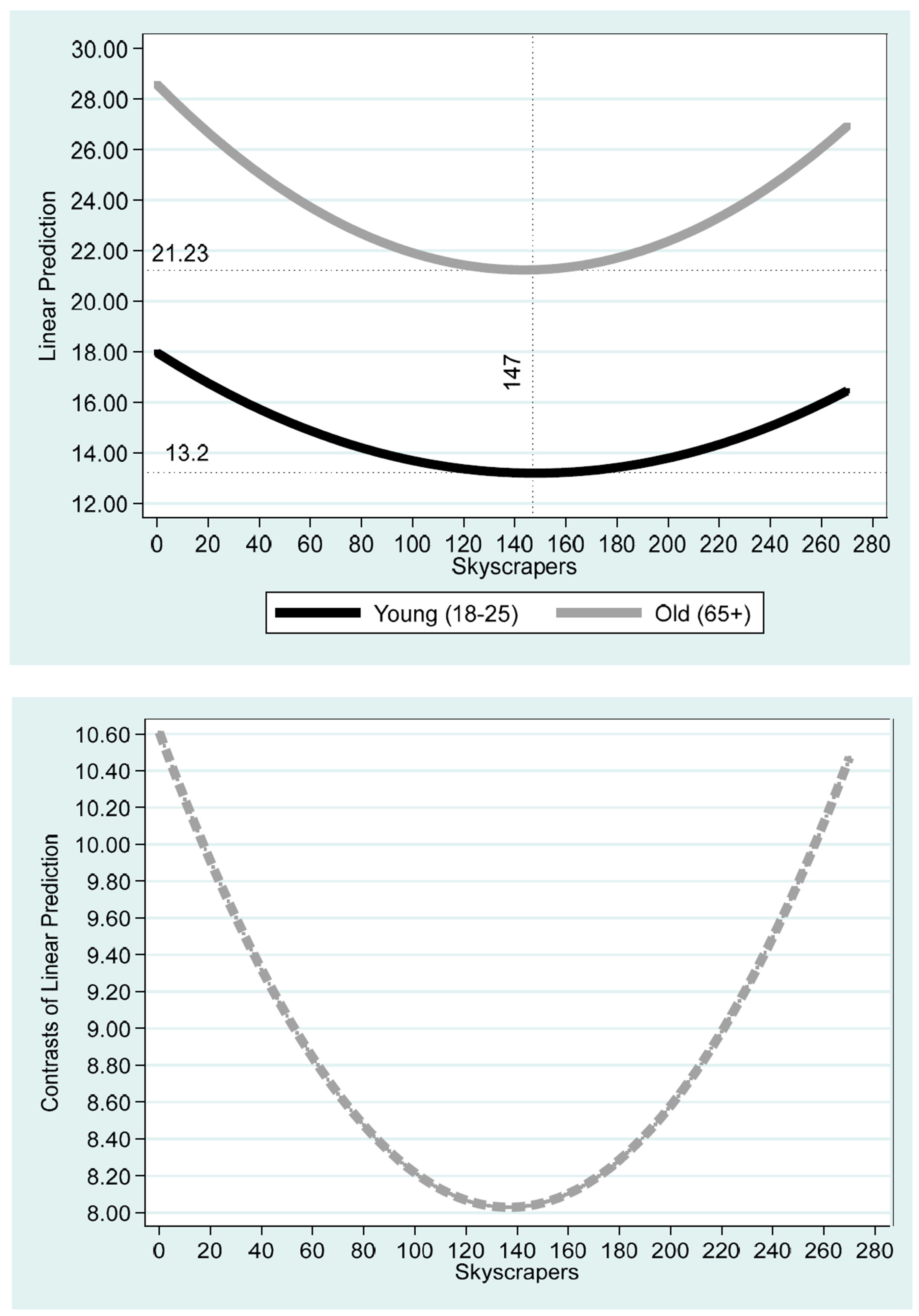
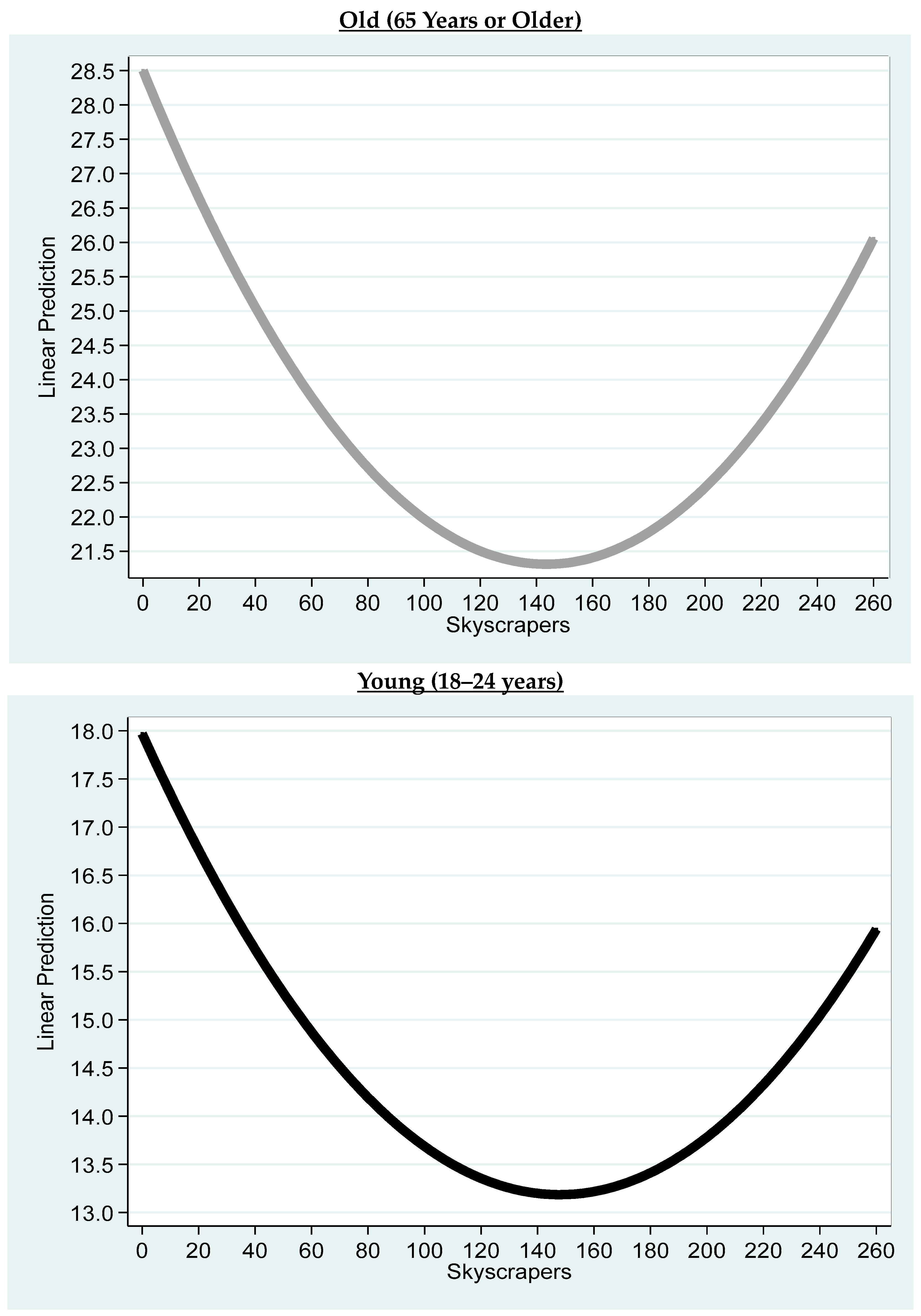
Table 2 reports the regression outcomes, based on which Figure 1 and Figure 2 are obtained. The RESET specification test clearly supports the quadratic specification given by Equation (1) (F(3, 918) = 1.16; p = 0.3220). The top part of Figure 1 describes the projected obesity prevalence as a function of the number of skyscrapers in the state and is stratified by age cohort to young—aged between 18 and 25 years—and old—aged above 65 years. The bottom part of Figure 1 describes the difference in the projected obesity prevalence between the old and the young cohorts as a function of the number of skyscrapers in the state.
For both age cohorts, a U-shaped curve was obtained. According to Figure 1, for the old (young) age cohort, the projected obesity prevalence is 17.96% (28.57%) where the number of skyscrapers in the state is zero. The projected prevalence drops to a minimum of 21.23% (8.21%) for 144 (147) skyscrapers in the state and then rises to 16.44% (26.93%) for 270 skyscrapers in the state.
Table 2.
Regression analysis for the oldest vs. youngest age cohorts.
| Column (1) | |
|---|---|
| Variables | Obesity Prevalence |
| (Year − 2011) | 0.514 *** |
| (<0.01) | |
| Skyscrapers×Skyscrapers | 0.000218 *** |
| (1.43 × 10⁻⁶) | |
| Old ×Skyscrapers×Skyscrapers | 0.000138 ** |
| (0.0458) | |
| Skyscrapers | −0.0645 *** |
| (5.62 × 10⁻⁹) | |
| Old ×Skyscrapers | −0.0377 ** |
| (0.0348) | |
| Old | 10.61 *** |
| (<0.01) | |
| Constant | 15.63 *** |
| (<0.01) | |
| Observations | 928 |
| R squared | 0.708 |
| p value RESET Test | 0.3220 |
| Minimum Young (18–25) | |
| Skyscrapers | 147 [126, 170] |
| Projected Prevalence of Obesity | 13.2 [11.87, 14.52] |
| Minimum Old (66+) | |
| Skyscrapers | 144 [137, 150] |
| Projected Prevalence of Obesity | 21.23 [19.48, 22.99] |
| Minimum Old–Young Differences | 8.21 [5.83, 10.25] |
| Maximum Old–Young Differences | 10.61 [10.06, 11.13] |
Notes: The Old variable receives 1 for old age above 65 years and zero for young cohort between 18–25 years. The Ramsey’s RESET (Regression Specification Error Test—see Ramanathan, 2002 [54] (pp. 270–271)) procedure is based on two steps. The first step of the procedure is the construction of vector of predictions () from the model given in Equation (1). The second step is the incorporation of , , and in Equation (1) as additional independent variables and testing of the joint null hypothesis that their coefficients equal zero. If the null hypothesis is not rejected, one could argue that the model specification is appropriate. According to this procedure, the null hypothesis is not rejected (F(3, 918) = 1.16; p = 0.3220). Robust p values are given in parentheses. The 5% confidence intervals are given in square brackets. ** p < 0.05; *** p < 0.01.
Figure 1.
Impact of skyscrapers on the prevalence of obesity: young vs. old. Notes: Based on the regression outcomes reported in Table 2. The vertical axis of the top (bottom) figure is the projected prevalence of obesity (young–old differences in obesity prevalence in the state). The horizonal axis is the number of skyscrapers in the state.

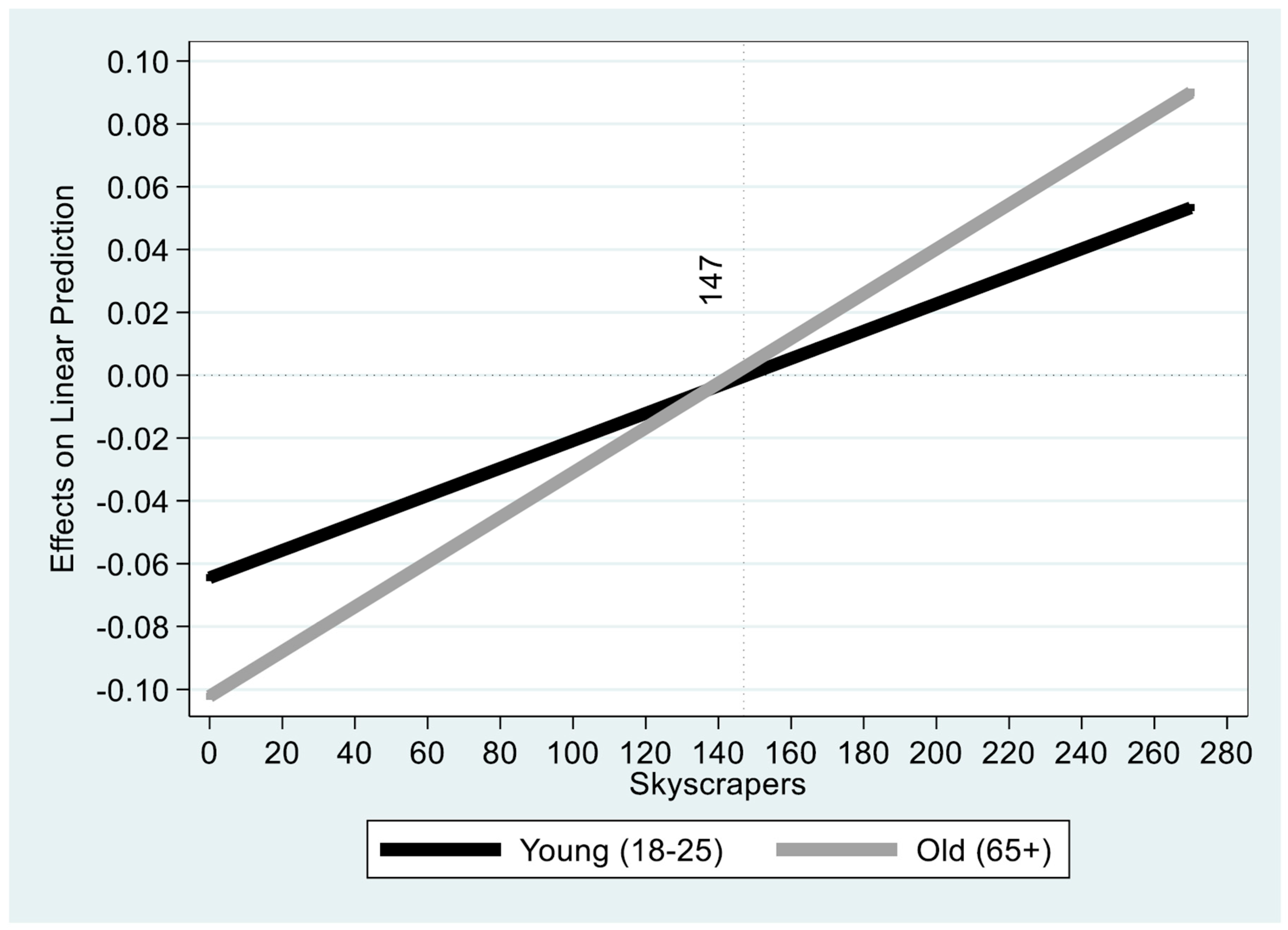
Figure 2.
Incremental change in projected prevalence of obesity: young vs. old. Notes: Based on the regression outcomes reported in Table 2. The graph demonstrates the incremental change for each number of skyscrapers.
Figure 2.
Incremental change in projected prevalence of obesity: young vs. old. Notes: Based on the regression outcomes reported in Table 2. The graph demonstrates the incremental change for each number of skyscrapers.

It is evident from Table 2 that the coefficients of both of the interaction variables, Old ×Skyscrapers×Skyscrapers (p < 0.0458) and Old ×Skyscrapers (p < 0.0348), are statistically different from zero. In addition, the coefficient of the Old variable is statistically different from zero (p < 0.01). The implications manifested at the bottom part of Figure 1 are a lower projected obesity prevalence in favor of the young age cohort by a minimum of 8.21% (95% confidence interval of [5.83%, 10.25%]) and a maximum of 10.61% (95% confidence interval of [10.06%, 11.13%]) for each number of skyscrapers.
Finally, Figure 2 gives the incremental change in the projected prevalence of obesity for both age cohorts (young vs. old). As can be seen from the figure, between 0 and 147 skyscrapers (the falling domain of the projected obesity prevalence), the drop in the incremental projected obesity prevalence for the old age cohort with each additional skyscraper is higher. This trend is reversed for the rising domain of between 147 and 270 skyscrapers.
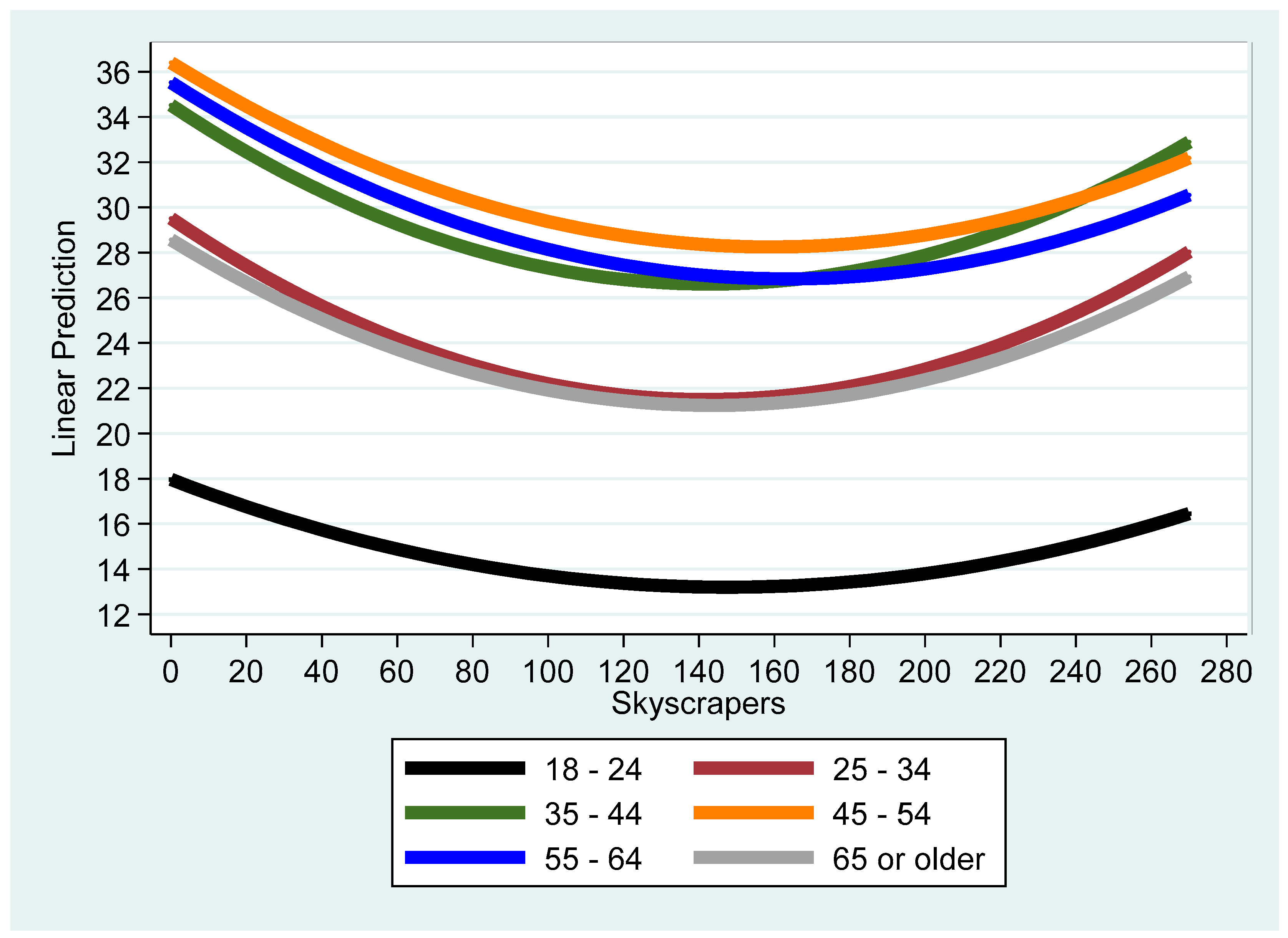
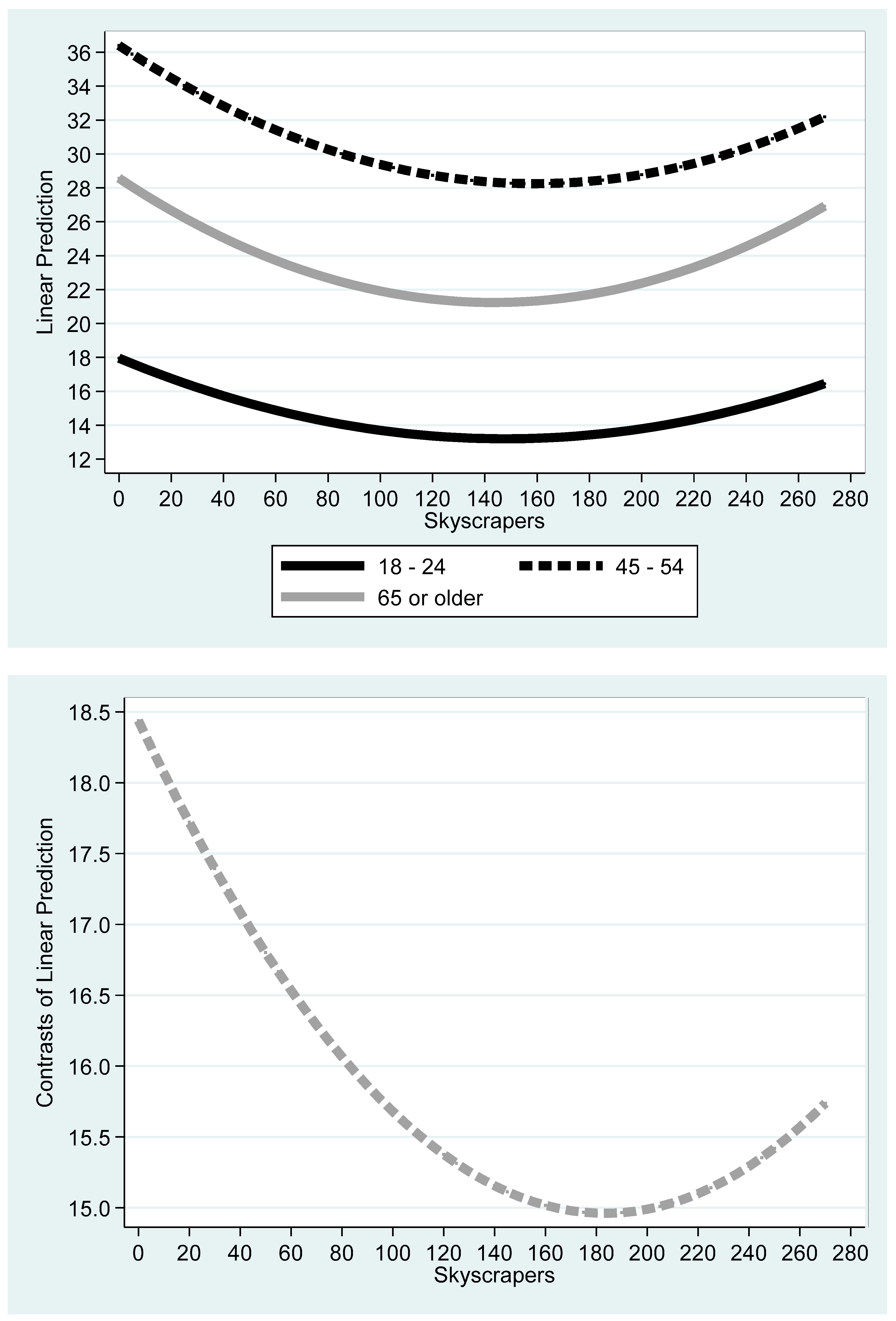
A further extension of the model is the inclusion of the obesity prevalence as the dependent variable and all age cohorts as independent dummy variables, where the baseline is the youngest age cohort (18–24). Additional explanatory variables are the age cohort dummy variables interacted with the (squared) number of skyscrapers. The coefficients of the model were estimated by the conventional OLS procedure. Given that the interpretation of the outcomes is very complex, we simplified the exposition by providing appropriate figures based on the outcomes obtained. Column (1) of Table 3 reports the regression outcomes and Figure 3—the derived graph of the projected obesity prevalence vs. number of skyscrapers for all age cohorts. According to this figure, the age cohort with the lowest (highest) projected obesity prevalence for every number of skyscrapers is the 18–25 (45–54) cohorts. Consequently, column (2) of Table 3 reports the results of three age cohorts—(18–24—the youngest with the lowest projected obesity prevalence; 45–54—with the highest projected obesity prevalence; and 65 or older—the oldest age cohorts).
Table 3.
Regression analysis for all age cohorts.
| Column (1) | Column (2) | |
|---|---|---|
| Variables | Obesity_Prevalence | Obesity_Prevalence |
| (Year − 2011) | 0.553 *** | 0.583 *** |
| (<0.01) | (<0.01) | |
| Skyscrapers×Skyscrapers | 0.000218 *** | 0.000218 *** |
| (1.28 × 10⁻⁶) | (1.38 × 10⁻⁶) | |
| age_25_34× Skyscrapers×Skyscrapers | 0.000180 ** | - |
| (0.0150) | - | |
| age_35_44× Skyscrapers×Skyscrapers | 0.000170 ** | - |
| (0.0187) | - | |
| age_45_54× Skyscrapers×Skyscrapers | 0.000103 * | 0.000103 * |
| (0.0859) | (0.0862) | |
| age_55_64× Skyscrapers×Skyscrapers | 0.000108 | - |
| (0.102) | - | |
| age_65_or_older× Skyscrapers×Skyscrapers | 0.000138 ** | 0.000138 ** |
| (0.0459) | (0.0466) | |
| Skyscrapers | −0.0644 *** | −0.0644 *** |
| (4.32 × 10⁻⁹) | (4.88 × 10⁻⁹) | |
| age_25_34× Skyscrapers | −0.0485 *** | - |
| (0.00862) | - | |
| age_35_44× Skyscrapers | −0.0464 ** | - |
| (0.0103) | - | |
| age_45_54× Skyscrapers | −0.0379 ** | −0.0379 ** |
| (0.0120) | (0.0121) | |
| age_55_64× Skyscrapers | −0.0420 ** | - |
| (0.0124) | - | |
| age_65_or_older× Skyscrapers | −0.0377 ** | −0.0377 ** |
| (0.0348) | (0.0352) | |
| Constant | 15.46 *** | 15.32 *** |
| (<0.01) | (<0.01) | |
| age_25_34 | 11.55 *** | - |
| (<0.01) | - | |
| age_35_44 | 16.56 *** | - |
| (<0.01) | - | |
| age_45_54 | 18.44 *** | 18.44 *** |
| (<0.01) | (<0.01) | |
| age_55_64 | 17.56 *** | - |
| (<0.01) | - | |
| age_65_or_older | 10.61 *** | 10.61 *** |
| (<0.01) | (<0.01) | |
| Observations | 2784 | 1392 |
| R squared | 0.723 | 0.806 |
| F values | 419.5 *** | 575.9 *** |
| D.F. Numerator | 18 | 9 |
| D.F. Denominator | 2765 | 1382 |
| Critical F value | 1.94 | 2.42 |
Notes: Robust p values are given in parentheses. * p < 0.1; ** p < 0.05; *** p < 0.01.
Figure 3.
All age cohorts. Notes: The figure describes projected obesity prevalence in percentage points of all age cohorts as a function of the number of skyscrapers and is based on the regression outcomes applied to 2784 observations and given in column (1) of Table 3.
Figure 3.
All age cohorts. Notes: The figure describes projected obesity prevalence in percentage points of all age cohorts as a function of the number of skyscrapers and is based on the regression outcomes applied to 2784 observations and given in column (1) of Table 3.

The top part of Figure 4 gives the derived graph of the three age cohorts. The bottom part refers to the difference between the 18–24 and 45–54 age cohorts for each number of skyscrapers. Unlike the youngest and oldest groups, and given the high workload during the lifespan dedicated to work, there is presumably a lack of available time to exercise and think of a healthy diet among the 45–54 age cohorts.
Figure 4.
Obesity prevalence vs. number of skyscrapers: three age cohorts. Notes: The top figure describes projected obesity prevalence in percentage points of three age cohorts (18–24—the youngest with the lowest projected obesity prevalence; 45–54—with the highest projected obesity prevalence; 65 or older—the oldest age cohorts) as a function of the number of skyscrapers. Projections are based on the regression outcomes applied to 1392 observations and given in column (2) of Table 3. The bottom figure refers to the difference between 18–24 and 45–54 age cohorts for each number of skyscrapers.

4. Robustness Test
To further support the outcomes and validate the empirical model of young vs. old populations, the objective of the current section is to run a series of robustness tests. We ran two types of robustness tests. The first type is designed to use the panel structure and run random effect regressions for the old and young age cohort separately. The second type is designed to test the cross validation of the empirical model.
We used the panel structure for each group separately (old and young) to run a random effect regression. The outcomes of this procedure are given in Table 4 and Figure 5.
The random effect regression accounts for serial correlation between the vector of generic components (—the dummy variables for the US states) and the time variable due to the fact that the same state appears in consecutive years. Described differently, if ( is the classical random disturbance term), the random effect procedure accounts for the parameter (—the respective variances—and T—the time variable), that reflects serial correlation. (Wooldridge [48], 2009: 489–490). Following the random effect regression, the conventional model becomes where reflects the cross-sectional average, and . (Wooldridge, 2009 [48] (pp. 489–490)). The results remain robust with respect to the simple OLS procedure.
Finally, to further establish the relationships between the variables, we ran cross validation tests (Table 4 and Table 5 below). The cross validate procedure can be carried out on cross-sectional datasets only due to the random sampling procedure. The latter is not reasonable within the framework of time series analysis where data are organized in ascending chronological order. The procedure creates a vector of predictions denoted as , where each of the five folds randomly assigns a subset of the off-sample group and runs an OLS regression on the training of the on-sample group. The vector contains only predictions from the off-sample group. Table 5 gives the Pearson correlations between the obesity prevalence and and includes five rounds of this repetitive procedure. The outcomes demonstrate high Pearson correlations (stretches between 0.3357—the lowest—and 0.6901—the highest) and rejection of the null hypothesis of zero correlation in all cases at the 1% level.
Likewise, the cross fold procedure can be carried out on cross-sectional datasets only. Recall that time series data are organized in ascending chronological order. Consequently, random sampling procedures are not consistent with the data structure. The procedure creates a vector of predictions, where each of the five folds randomly assigns a subset of the off-sample group and runs an OLS regression on the training of the on-sample group. Table 6 gives the pseudo-R squared as a goodness-of-fit measure. The outcomes show that this measure spans between 0.0598 (lowest) and 0.6849 (highest).
Table 5.
Cross validation for young vs. old populations.
| Round | 2011 | 2012 | 2013 | 2014 | 2015 | 2016 | 2017 | 2018 | 2019 | 2020 | Total |
|---|---|---|---|---|---|---|---|---|---|---|---|
| First | 0.6557 *** | 0.4887 *** | 0.3830 *** | 0.4911 *** | 0.4414 *** | 0.4927 *** | 0.6363 *** | 0.3559 *** | 0.4096 *** | 0.5428 *** | |
| Second | 0.6582 *** | 0.4875 *** | 0.3858 *** | 0.4872 *** | 0.4380 *** | 0.4641 *** | 0.6901 *** | 0.3564 *** | 0.4158 *** | 0.5518 *** | |
| Third | 0.6812 *** | 0.4880 *** | 0.3830 *** | 0.4886 *** | 0.4297 *** | 0.4755 *** | 0.6313 *** | 0.3433 *** | 0.4170 *** | 0.5976 *** | |
| Fourth | 0.6625 *** | 0.5342 *** | 0.3835 *** | 0.4916 *** | 0.4632 *** | 0.5000 *** | 0.6405 *** | 0.3718 *** | 0.3980 *** | 0.5657 *** | |
| Fifth | 0.6646 *** | 0.4797 *** | 0.3357 *** | 0.4866 *** | 0.4400 *** | 0.4950 *** | 0.6900 *** | 0.3446 *** | 0.4021 *** | 0.5726 *** | |
| Obs. | 90 | 90 | 92 | 94 | 94 | 94 | 94 | 94 | 92 | 94 | 928 |
Notes: The cross validate procedure can be carried out on cross-sectional datasets only. The procedure creates a vector of predictions denoted as , where each of the five folds randomly assigns a subset of off-sample group and runs an OLS regression on the training of on-sample group. The vector contains only predictions from the off-sample group. The table gives the Pearson correlations between obesity prevalence and . *** p < 0.01 for the rejection of the null hypothesis of zero correlation.
5. Discussion
We investigated the association between obesity prevalence, the time variable, and the number of skyscrapers as proxies for urban environments and age cohorts. The data employed in this study refers to the obesity prevalence at a US statewide level in 2011–2020 obtained from the Center for Disease Control and Prevention (CDC website [18]). To examine the possibility of nonmonotonic patterns, we used the quadratic model. The outcomes of this study showed U-shaped curves for both the old and young populations with a minimum point of 147 skyscrapers. The minimal obesity prevalence was 21.23 percent among the old population and 13.2 percent among the young population.
The public policy outcome of our study is the need to implement different recommendations in dissimilar urban environments based on age cohort stratification. One possible example is the construction of more retirement homes for the old population when the number of skyscrapers is below 147 and student dormitories for the young population when the number of skyscrapers is above 147. One might consider the possibility to propose subsidized residence in these regions, where the ability to exploit the urban infrastructure (at least according to our results) is the highest. Yet, urban planners should weigh these along with other considerations.
In the residential areas of older people, it is advised to encourage a healthier diet—this should also be considered in terms of business licensing to restaurants. Extreme care will be required for the types of sports facilities found in those areas. Priority should be given to areas where there are young people for accelerated activity such as running, cycling, and ball games. On the other hand, in areas with a high concentration of adults, the counting infrastructure could be adjusted accordingly: walking paths, bowling, and benches for sitting. (For more general guidelines for avoiding or reducing obesity prevalence, see, for example, ref. [57] and Appendix A).
One limitation of this article concerns the grid of data at a US statewide level. One could argue that if the aim is to investigate the impact of urban environments, statewide data is not the correct grid. Yet, many articles employed data at either a US statewide or county levels, including the following: [15,21,58] (Urban Studies and Health); [59,60] (Medicine); [61] (Genetics); [62] (Endocrinology, Diabetes and Metabolism); and [63] (Clinical Psychology).
However, even if we accept this criticism, there still remains an open question of what the appropriate grid is to investigate the impact of urban and non-urban environments.
In their review, Anas, Arnott and Small [64] discussed the question of how to describe the urban spatial structure. According to authors, “A more recent approach to describing urban spatial patterns is on the idea that they resemble fractals, geometric figures which display ever finer structures when viewed as finer resolutions. Mathematically, a fractal is the limiting result of repeatedly replicated, at smaller and smaller measured length with respect to resolution is called as the fractal dimension.” (page 1432 italics appears as in the source). In addition, they state, “More significantly, one can use fractals to represent two-dimensional development patterns, thereby capturing irregularities in the interior as well as at the boundary of the developed area. For example, a fractal can be generated mathematically by starting with a large filled-in square, then selectively deleting to smaller and smaller squares so as to create self-similar patterns at smaller and smaller scales.” (page 1432).
Described differently, according to this approach, each chosen grid is somewhat arbitrary. Another support is given in [21] and [58]. In the limitation subsection of Ewing et al. [21], for instance, state that: “This study relates health to the built environment at the county scale, which is large compared to the living and working environments of most residents (Black and Macinko, 2008 [65]; Feng et al., 2010 [66]). Geocodes are only available from BRFSS down to the county level. If environmental effects are felt most strongly at the community or neighborhood scale, these results may understate the effects of the built environment on health (Booth et al., 2005 [67], p. 125)”.
Hamidi et al. [58] argue that: “Large metropolitan areas tend to have higher peak and average densities due to higher land rents, though with many exceptions. Contrast Boston with Atlanta, San Francisco and Houston.” (page 2).
6. Summary and Conclusions
This study investigated the impact of the more densely populated urban environment proxied by the number of skyscrapers on the obesity prevalence among young vs. old populations at a US Statewide level.
We employed a quadratic model, which relaxes the a priori assumption of monotonic rise or drop in obesity prevalence with the number of skyscrapers (for a discussion see, for example, ref. [50] (pp. 229–231)). The outcomes demonstrated a U-shaped curve, as well as a sharper decrease (increase) in the projected obesity prevalence with the number of skyscrapers in the range of 0–147 (147–270) skyscrapers for the old population age cohorts above 65 years. From a public policy perspective and given the long series of health problems associated with obesity, according to these outcomes, the optimal urban environments are the ones which reduce the projected obesity prevalence to a minimum, namely, with 144–147 skyscrapers.
Future research should focus on other age cohorts. Obesity gaps among these cohorts warrant additional research. The larger obesity gaps were obtained between the young (18–25) and the 45–54 age cohort where work productivity is the highest. Consequently, we extended the article and compared these groups as well. Yet, based on the obesity criteria, the age cohorts may be classified into three groups: (1) The youngest age cohort (18–25) presents the lowest level of obesity prevalence. Presumably, this group has the highest awareness of obesity, and physical activity and genetics work in their favor. (2) The age cohorts 25–34 and above 65 present medium levels of obesity prevalence. While the former group still has a high awareness of obesity and physical activity, the latter group has more available time for physical activity. )3) The rest of the age cohorts (35–44; 45–54; and 54–65) display the highest level of obesity prevalence. Given the high workload during the lifespan dedicated to work, there is presumably a lack of available time to exercise and think of a healthy diet.
The motivation types (intrinsic vs. extrinsic) are another subject for future research. These should be carried out with appropriate surveys in rural vs. urban communities. One example for urban investigation is Firestone et al. [46]. The authors investigated adult New Yorkers during 2010–2011. The authors found overall that 70.6% of adult New Yorkers reported having physically active friends. Having active friends was associated with increased leisure time for physical activity by a factor of two times more activity (56 min/week) for men and two and a half times more activity (35 min/week) for women. Physically active males and females who usually engaged in leisure time activities as a part of a group reported 1.4 times more activity than those who exercised alone.
Author Contributions
Y.A. (Yuval Arbel) contributed to the study conception and design, data collection and analysis, the first draft, and comments on previous versions of the manuscript. Y.A. (Yifat Arbel) contributed to the study conception and design, data collection and analysis, the first draft, and comments on previous versions of the manuscript. A.K. contributed to the study conception and design, data collection and analysis, the first draft, and comments on previous versions of the manuscript. M.K. contributed to the study conception and design, data collection and analysis, the first draft, and comments on previous versions of the manuscript. All authors have read and agreed to the published version of the manuscript.
Funding
This research received no external funding.
Institutional Review Board Statement
This research does not require IRB approval, since it does not involve any experiment or manipulation of subjects. All authors read and approved the final manuscript for submission.
Informed Consent Statement
Not applicable.
Data Availability Statement
The datasets used and/or analyzed during the current study are available from the corresponding author upon reasonable request.
Acknowledgments
The authors are grateful to Avishay Aiche, Chaim Fialkoff, Vincente Royuela and the participants of the 62nd ERSA congress in Alicante, Spain for helpful comments.
Conflicts of Interest
None of the authors have potential conflict of interest, financially or nonfinancially, nor directly or indirectly related to this work.
Abbreviations
| BMI | Body Mass Index |
| MVPA | Medium-to-Vigorous Physical Activity |
| PA | Physical Activity |
| RESET | Regression Specification Error Test |
| SDT | Self-Determination Theory |
| WHO | World Health Organization |
| WHR | Waist–Hip Ratio |
Appendix A. Core Elements and Related Topics and Activities in the CRI LEP
| Core Elements | Selected Examples of Topics and Activities |
|---|---|
| Nutrition |
|
| Physical Activity |
|
| Behavior Change |
|
| Sense of Purpose |
|
| Integrative Health |
|
| Social Support and Follow-up Services |
|
References
- Glaeser, E. Cities, Productivity, and Quality of Life. Science 2011, 333, 592–594. [Google Scholar] [CrossRef] [PubMed]
- Glaeser, E. Triumph of the City: How Our Greatest Invention Makes Us Richer, Smarter, Greener, Healthier, and Happier; Penguin Books: New York, NY, USA, 2011. [Google Scholar]
- Glaeser, E. Viewpoint: Triumph of the city. J. Transp. Land Use 2012, 5, 1–4. [Google Scholar] [CrossRef]
- Mills, E.S. An Aggregative Model of Resources Allocation in a Metropolitan Area. Am. Econ. Rev. 1967, 57, 197. [Google Scholar]
- O’Sullivan, A. Urban Economics, 8th ed.; McGraw Hills International Edition: Singapore, 2012. [Google Scholar]
- Alonso, W. A Model of the Urban Land Market: Location and Densities of Dwellings and Businesses. Ph.D. Dissertation, University of Pennsylvania, Philadelphia, PA, USA, 1960. [Google Scholar]
- Alonso, W. Location and Land Use; Harvard University Press: Cambridge, MA, USA, 1964. [Google Scholar]
- Muth, R. Cities and Housing; University of Chicago Press: Chicago, IL, USA, 1969. [Google Scholar]
- McDonald, J.F.; McMillen, D.P. Urban Economics and Real Estate: Theory and Policy, 2nd ed.; John Wiley & Sons Incorporated: Hoboken, NJ, USA, 2011. [Google Scholar]
- McDonald, J.F. William Alonso, Richard Muth, Resources for the Future, and the Founding of Urban Economics. J. Hist. Econ. Thought 2007, 29, 67–84. [Google Scholar] [CrossRef]
- Mills, E.S.; Hamilton, B.W. Urban Economics, 4th ed.; Harper Collins College Publishers: New York, NY, USA, 1989. [Google Scholar]
- Arbel, Y.; Fialkoff, C.; Kerner, A. Climate Change and Housing Choice: The Impact of Climate Differences on Capital-Land Elasticity of Substitution. J. Real Estate Lit. 2018, 26, 191–209. [Google Scholar] [CrossRef]
- Arbel, Y.; Fialkoff, C.; Kerner, A. The Association of Pension Income with the Incidence of Type I Obesity among Retired Israelis. J. Obes. 2019, 2019, 5101867. [Google Scholar] [CrossRef] [PubMed]
- Arbel, Y.; Fialkoff, C.; Kerner, A. The Chicken and Egg Problem: Obesity and the Urban Monocentric Model. J. Real Estate Financ. Econ. 2020, 61, 576–606. [Google Scholar] [CrossRef]
- Arbel, Y.; Arbel, Y.; Kerner, A.; Kerner, M. Do high-rise buildings influence melanoma? Tall buildings as positive externalities. Cities 2022, 131, 104002. [Google Scholar] [CrossRef]
- World Health Organization (WHO). June 2021: Obesity and Overweight. Available online: https://www.who.int/news-room/fact-sheets/detail/obesity-and-overweight (accessed on 10 October 2022).
- Zaccardi, F.; Franks, P.W.; Dudbridge, F.; Davies, M.J.; Khunti, K.; Yates, T. Mortality risk comparing walking pace to handgrip strength and a healthy lifestyle: A UK Biobank study. Eur. J. Prev. Cardiol. 2021, 28, 704–712. [Google Scholar] [CrossRef] [PubMed]
- Frank, L.D.; Iroz-Elardo, N.; MacLeod, K.E.; Hong, A. Pathways from built environment to health: A conceptual framework linking behavior and exposure-based impacts. J. Transp. Health 2019, 12, 319–335. [Google Scholar] [CrossRef]
- National Research Council (US); Committee on Physical Activity, Transportation, Land Use, Transportation Research Board; Institute of Medicine. Does the Built Environment Influence Physical Activity? Examining the Evidence—Special Report 282; Transportation Research Board: Washington, DC, USA, 2015; Volume 282.
- Ewing, R.; Meakins, G.; Hamidi, S.; Nelson, A.C. Relationship between urban sprawl and physical activity, obesity, and morbidity—Update and refinement. Health Place 2014, 26, 118–126. [Google Scholar] [CrossRef] [PubMed]
- Mulalic, I.; Rouwendal, J. Does improving public transport decrease car ownership? Evidence from a residential sorting model for the Copenhagen metropolitan area Reg. Sci. Urban Econ. 2020, 83, 103543. [Google Scholar] [CrossRef]
- World Health Organization (WHO): Physical Activity. 2022. Available online: https://www.who.int/news-room/fact-sheets/detail/physical-activity (accessed on 10 October 2023).
- Winston, T.N. Handbook on Burnout and Sleep Deprivation: Risk Factors, Management Strategies and Impact on Performance and Behavior; Nova Science Publishers, Inc.: Hauppauge, NY, USA, 2015. [Google Scholar]
- Fatima, Y.; Doi, S.A.R.; Mamun, A.A. Longitudinal impact of sleep on overweight and obesity in children and adolescents: A systematic review and bias-adjusted meta-analysis. Obes. Rev. 2015, 16, 137–149. [Google Scholar] [CrossRef]
- Mayne, S.L.; Morales, K.H.; Williamson, A.A.; Grant, S.F.A.; Fiks, A.G.; Basner, M.; Dinges, D.F.; Zemel, B.S.; Mitchell, J.A. Associations of the residential built environment with adolescent sleep outcomes. Sleep 2021, 44, zsaa276. [Google Scholar] [CrossRef] [PubMed]
- Chen, P.; Zhou, J. Effects of the built environment on automobile-involved pedestrian crash frequency and risk. J. Transp. Health 2016, 3, 448–456. [Google Scholar] [CrossRef]
- Feuillet, T.; Salze, P.; Charreire, H.; Menai, M.; Enaux, C.; Perchoux, C.; Hess, F.; Kesse-Guyot, E.; Hercberg, S.; Simon, C.; et al. Built environment in local relation with walking: Why here and not there? J. Transp. Health 2016, 3, 500–512. [Google Scholar] [CrossRef]
- Nigg, C.; Oriwol, D.; Wunsch, K.; Burchartz, A.; Kolb, S.; Worth, A.; Woll, A.; Niessner, C. Population density predicts youth’s physical activity changes during COVID-19—Results from the MoMo study. Health Place 2021, 70, 102619. [Google Scholar] [CrossRef]
- Hino, K.; Asami, Y. Change in walking steps and association with built environments during the COVID-19 state of emergency: A longitudinal comparison with the first half of 2019 in Yokohama, Japan. Health Place 2021, 69, 102544. [Google Scholar] [CrossRef]
- Handy, S.; Cao, X.; Mokhtarian, P.L. Self-Selection in the Relationship between the Built Environment and Walking: Empirical Evidence from Northern California. J. Am. Plan. Assoc. 2006, 72, 55–74. [Google Scholar] [CrossRef]
- Sun, G.; Oreskovic, N.M.; Lin, H. How do changes to the built environment influence walking behaviors? A longitudinal study within a university campus in Hong Kong. Int. J. Health Geogr. 2014, 13, 28–37. [Google Scholar] [CrossRef]
- Chaix, B.; Simon, C.; Charreire, H.; Thomas, F.; Kestens, Y.; Karusisi, N.; Vallée, J.; Oppert, J.-M.; Weber, C.; Pannier, B. The environmental correlates of overall and neighborhood based recreational walking (a cross-sectional analysis of the RECORD Study). Int. J. Behav. Nutr. Phys. Act. 2014, 11, 20. [Google Scholar] [CrossRef] [PubMed]
- Wasfi, R.A.; Dasgupta, K.; Eluru, N.; Ross, N.A. Exposure to walkable neighbourhoods in urban areas increases utilitarian walking: Longitudinal study of Canadians. J. Transp. Health 2016, 3, 440–447. [Google Scholar] [CrossRef]
- Beales, P.R.; Farooqi, I.S.; O’Rahilly, S. Genetics of Obesity Syndromes; Oxford University Press: Oxford, UK, 2009. [Google Scholar]
- Sallis, J.F.; Cerin, E.; Conway, T.L.; Adams, M.A.; Frank, L.D.; Pratt, M.; Salvo, D.; Schipperijn, J.; Smith, G.; Cain, K.L.; et al. Physical activity in relation to urban environments in 14 cities worldwide: A cross-sectional study. Lancet 2016, 387, 2207–2217. [Google Scholar] [CrossRef] [PubMed]
- Kim, B.Y.; Choi, D.H.; Jung, C.H.; Kang, S.K.; Mok, J.O.; Kim, C.H. Obesity and Physical Activity. J. Obes. Metab. Syndr. 2017, 26, 15–22. [Google Scholar] [CrossRef] [PubMed]
- Lee, A.; Cardel, M.; Donahoo, W.T. Social and Environmental Factors Influencing Obesity. In Endotext [Internet]; Feingold, K.R., Anawalt, B., Boyce, A., Chrousos, G., de Herder, W.W., Dhatariya, K., Dungan, K., Grossman, A., Hershman, J.M., Hofland, J., Eds.; MDText.com, Inc.: South Dartmouth, MA, USA, 2019. Available online: https://0-www-ncbi-nlm-nih-gov.brum.beds.ac.uk/books/NBK278977/ (accessed on 10 October 2023).
- Allender, S.; Cowburn, G.; Foster, C. Understanding participation in sport and physical activity among children and adults: A review of qualitative studies. Health Educ. Res. 2006, 21, 826–835. [Google Scholar] [CrossRef] [PubMed]
- Roberts, G.C.; Nerstad, C.G.L.; Lemyre, P.N. Motivation in Sport and Performance. Oxf. Res. Encycl. Psychol. 2018. [Google Scholar] [CrossRef]
- Ahmed, D.; Ho, W.K.Y.; Al-Haramlah, A.; Mataruna-Dos-Santos, L.J. Motivation to participate in physical activity and sports: Age transition and gender differences among India’s adolescents. Cogent Psychol. 2020, 7, 1798633. [Google Scholar] [CrossRef]
- Kalajas-Tilga, H.; Koka, A.; Hein, V.; Tilga, H.; Raudsepp, L. Motivational processes in physical education and objectively measured physical activity among adolescents. J. Sport Health Sci. 2020, 9, 462–471. [Google Scholar] [CrossRef] [PubMed]
- Ahmadi, A.; Noetel, M.; Parker, P.; Ryan, R.M.; Ntoumanis, N.; Reeve, J.; Beauchamp, M.; Dicke, T.; Yeung, A.; Ahmadi, M.; et al. A classification system for teachers’ motivational behaviors recommended in self-determination theory interventions. J. Educ. Psychology. 2023. [Google Scholar] [CrossRef]
- Molanorouzi, K.; Khoo, S.; Morris, T. Motives for adult participation in physical activity: Type of activity, age, and gender. BMC Public Health 2015, 15, 66. [Google Scholar] [CrossRef]
- Young, B.W.; Callary, B.; Rathwell, S. Psychological Considerations for the Older Athlete. Oxf. Res. Encycl. Psychol. 2018. [Google Scholar] [CrossRef]
- Tsai, T.-H.; Wong, A.M.; Lee, H.-F.; Tseng, K.C. A Study on the Motivation of Older Adults to Participate in Exercise or Physical Fitness Activities. Sustainability 2022, 14, 6355. [Google Scholar] [CrossRef]
- Firestone, M.J.; Yi, S.S.; Bartley, K.F.; Eisenhower, D.L. Perceptions and the role of group exercise among New York City adults, 2010–2011: An examination of interpersonal factors and leisure-time physical activity. Prev. Med. 2015, 72, 50–55. [Google Scholar] [CrossRef] [PubMed]
- Center for Disease Control and Prevention (CDC). Nutrition, Physical Activity, and Obesity: Data, Trends and Maps. Available online: https://nccd.cdc.gov/dnpao_dtm/rdPage.aspx?rdReport=DNPAO_DTM.ExploreByTopic&islClass=OWS&islTopic=&go=GO (accessed on 10 October 2023).
- Wooldridge, J.M. Introductory Econometrics: A Modern Approach, 4th ed.; International Student Edition; South Western CENGAGE Learning: Boston, MA, USA, 2009. [Google Scholar]
- Yin, C.; Sun, B. Does Compact Built Environment Help to Reduce Obesity? Influence of Population Density on Waist–Hip Ratio in Chinese Cities. Int. J. Environmental. Res. Public Health 2020, 17, 7746. [Google Scholar] [CrossRef] [PubMed]
- Chiang, A.; Wainwright, K. Fundamental Methods of Mathematical Economics, 4th ed.; McGraw Hills International Edition: Singapore, 2015. [Google Scholar]
- Lam, T.M.; Vaartjes, I.; Grobbee, D.E.; Karssenberg, D.; Lakerveld, J. Associations between the built environment and obesity: An umbrella review. Int. J. Health Geogr. 2021, 20, 1–24. [Google Scholar] [CrossRef]
- Ihle, A.; Gouveia, É.R.; Gouveia, B.R.; Zuber, S.; Mella, N.; Desrichard, O.; Cullati, S.; Oris, M.; Maurer, J.; Kliegel, M. The relationship of obesity predicting decline in executive functioning is attenuated with greater leisure activities in old age. Aging Ment. Health 2021, 25, 613–620. [Google Scholar] [CrossRef]
- Mathus-Vliegen, E.M.H. Prevalence, pathophysiology, health consequences and treatment options of obesity in the elderly: A guideline. Obes. Facts 2012, 5, 460–483. [Google Scholar] [CrossRef] [PubMed]
- Ramanathan, R. Introductory Econometrics with Applications, 5th ed.; South Western Thomson Learning: Mason, OH, USA, 2002. [Google Scholar]
- Greene, W.H. Econometric Analysis, 7th ed.; Pearson Education Limited: Sumas, WA, USA, 2012. [Google Scholar]
- OECD Obesity Update. 2017. Available online: https://www.oecd.org/health/obesity-update.htm (accessed on 10 October 2023).
- Pleasant, A. Assisting Vulnerable Communities: Canyon Ranch Institute’s and Health Literacy Media’s Health Literacy and Community-Based Interventions. In Health Literacy: New Directions in Research, Theory and Practice; Logan, R.A., Siegel, E.R., Eds.; IOS Press: Amsterdam, The Netherlands, 2017; pp. 127–164. [Google Scholar]
- Hamidi, S.; Ewing, R.; Sabouri, S. Longitudinal analyses of the relationship between development density and the COVID-19 morbidity and mortality rates: Early evidence from 1,165 metropolitan counties in the United States. Health Place 2020, 64, 102378. [Google Scholar] [CrossRef]
- Arbel, Y.; Arbel, Y.; Kerner, A.; Kerner, M. What is the optimal country for minimum COVID-19 morbidity and mortality rates? Environ. Sci. Pollut. Res. 2023, 30, 59212–59232. [Google Scholar] [CrossRef]
- Arbel, Y.; Arbel, Y.; Arbel, Y.; Kerner, A.; Kerner, M. Can reduction in infection and mortality rates from coronavirus be explained by an obesity survival paradox? An analysis at the US statewide level. Int. J. Obes. 2020, 44, 2339–2342. [Google Scholar] [CrossRef] [PubMed]
- Arbel, Y.; Arbel, Y.; Arbel, Y.; Kerner, A.; Kerner, M. Is obesity a risk factor for melanoma? BMC Cancer 2023, 23, 178. [Google Scholar] [CrossRef] [PubMed]
- Arbel, Y.; Arbel, Y.; Arbel, Y.; Kerner, A.; Kerner, M. Can Obesity Prevalence Explain COVID-19 Indicators (Cases, Mortality, and Recovery)? A Comparative Study in OECD Countries. J. Obes. 2022, 10, 4320120. [Google Scholar] [CrossRef] [PubMed]
- Arbel, Y.; Fialkoff, C.; Kerner, A.; Kerner, M. Can increased recovery rates from coronavirus be explained by prevalence of ADHD? An analysis at the US statewide level. J. Atten. Disord. 2021, 25, 1951–1954. [Google Scholar] [CrossRef] [PubMed]
- Anas, A.; Arnott, R.; Small, K.A. Urban Spatial Structure. J. Econ. Lit. 1998, 36, 1426–1464. [Google Scholar]
- Black, J.L.; Macinko, J. Neighborhood sand obesity. Nutr. Rev. 2008, 66, 2–20. [Google Scholar] [CrossRef] [PubMed]
- Feng, J.; Glass, T.; Curriero, F.; Stewart, W.; Schwartz, B. The built environment and obesity: A systematic review of the epidemiologic evidence. Health Place 2010, 16, 175–190. [Google Scholar] [CrossRef] [PubMed]
- Booth, K.M.; Pinkston, M.M.; Poston, W.S. Obesity and the built environment. J. Am. Diet Assoc. 2005, 105 (Suppl. S1), S110–S117. [Google Scholar] [CrossRef] [PubMed]
Figure 5.
Old vs. young in a panel framework. Notes: The upper (lower) figure is based on column 1 (2) in Table 4.
Figure 5.
Old vs. young in a panel framework. Notes: The upper (lower) figure is based on column 1 (2) in Table 4.

Table 4.
Random effect regressions.
| Column (1) | Column (2) | |
|---|---|---|
| Old | Young | |
| Variables | Obesity_prevalence | Obesity_prevalence |
| (Year − 2011) | 0.520 *** | 0.519 *** |
| (<0.01) | (<0.01) | |
| 0.000349 *** | 0.000219 * | |
| (0.00232) | (0.0912) | |
| Skyscrapers | −0.100 *** | −0.0647 ** |
| (0.000344) | (0.0409) | |
| Constant | 26.15 *** | 15.62 *** |
| (<0.01) | (<0.01) | |
| Observations | 464 | 464 |
| Number of State 1 | 47 | 47 |
| Wald Chi squared (3) | 402.69 *** | 147.57 *** |
| 2.6687 | 2.9673 | |
| 1.6121 | 2.6649 | |
| 0.7327 | 0.5535 |
Notes: The random effect regression accounts for serial correlation between the vector of generic components (—the dummy variables for the US states) and the time variable due to the fact that the same state appears in consecutive years. Described differently, if ( is the classical random disturbance term), the random effect procedure accounts for the parameter (—the respective variances—and T—the time variable), that reflects serial correlation. (Wooldridge [48] (pp. 489–490)). Following the random effect regression, the conventional model becomes where reflects the cross-sectional average, and . ([48] (pp. 489–490)). The Wald Chi squared (3) values are the calculated statistics for the regression significance. The p values are given in parentheses. * p < 0.1,** p < 0.05, *** p < 0.01.
Table 6.
Crossfold for young vs. old populations.
| Round | 2011 | 2012 | 2013 | 2014 | 2015 | 2016 | 2017 | 2018 | 2019 | 2020 | Total |
|---|---|---|---|---|---|---|---|---|---|---|---|
| First | 0.3254 | 0.6100 | 0.6411 | 0.5963 | 0.2833 | 0.1110 | 0.6158 | 0.6659 | 0.5780 | 0.5977 | |
| Second | 0.6284 | 0.6287 | 0.5897 | 0.0598 | 0.6427 | 0.6537 | 0.6605 | 0.1739 | 0.6205 | 0.1539 | |
| Third | 0.6849 | 0.3242 | 0.0799 | 0.6390 | 0.5038 | 0.4619 | 0.1327 | 0.3052 | 0.2493 | 0.6190 | |
| Fourth | 0.6525 | 0.2400 | 0.6571 | 0.6791 | 0.6834 | 0.6397 | 0.2350 | 0.6833 | 0.0235 | 0.6792 | |
| Fifth | 0.5958 | 0.6295 | 0.3456 | 0.6583 | 0.6332 | 0.6201 | 0.7326 | 0.6202 | 0.6611 | 0.6297 | |
| Obs. | 90 | 90 | 92 | 94 | 94 | 94 | 94 | 94 | 92 | 94 | 928 |
Notes: The crossfold procedure can be carried out on cross-sectional datasets only. The procedure creates a vector of predictions, where each of the five folds randomly assigns a subset of off-sample group and runs an OLS regression on the training of on-sample group. The table gives the pseudo-R squared as a goodness-of-fit measure.
Disclaimer/Publisher’s Note: The statements, opinions and data contained in all publications are solely those of the individual author(s) and contributor(s) and not of MDPI and/or the editor(s). MDPI and/or the editor(s) disclaim responsibility for any injury to people or property resulting from any ideas, methods, instructions or products referred to in the content. |
© 2023 by the authors. Licensee MDPI, Basel, Switzerland. This article is an open access article distributed under the terms and conditions of the Creative Commons Attribution (CC BY) license (https://creativecommons.org/licenses/by/4.0/).
Share and Cite
MDPI and ACS Style
Arbel, Y.; Arbel, Y.; Kerner, A.; Kerner, M. Young vs. Old Population: Does Urban Environment of Skyscrapers Create Different Obesity Prevalence? BioMed 2023, 3, 440-459. https://0-doi-org.brum.beds.ac.uk/10.3390/biomed3040036
AMA Style
Arbel Y, Arbel Y, Kerner A, Kerner M. Young vs. Old Population: Does Urban Environment of Skyscrapers Create Different Obesity Prevalence? BioMed. 2023; 3(4):440-459. https://0-doi-org.brum.beds.ac.uk/10.3390/biomed3040036
Chicago/Turabian StyleArbel, Yuval, Yifat Arbel, Amichai Kerner, and Miryam Kerner. 2023. "Young vs. Old Population: Does Urban Environment of Skyscrapers Create Different Obesity Prevalence?" BioMed 3, no. 4: 440-459. https://0-doi-org.brum.beds.ac.uk/10.3390/biomed3040036