
Detailed Error Analysis for a Fractional Adams Method on Caputo–Hadamard Fractional Differential Equations


Department of Physical, Mathematical and Engineering, University of Chester, Chester CH1 4BJ, UK
*
Author to whom correspondence should be addressed.
†
These authors contributed equally to this work.
Foundations 2022, 2(4), 839-861; https://0-doi-org.brum.beds.ac.uk/10.3390/foundations2040057
Submission received: 28 August 2022
/
Revised: 12 September 2022
/
Accepted: 13 September 2022
/
Published: 22 September 2022
(This article belongs to the Special Issue Recent Advances in Fractional Differential Equations and Inclusions)
Abstract
:We consider a predictor–corrector numerical method for solving Caputo–Hadamard fractional differential equation over the uniform mesh with , where is a partition of . The error estimates under the different smoothness properties of the solution y and the nonlinear function f are studied. Numerical examples are given to verify that the numerical results are consistent with the theoretical results.
1. Introduction
Fractional differential equations have recently become an active research area due to the applications in fields including mechanics, computer science, and biology [1,2,3,4]. There are different fractional derivatives, e.g., Caputo, Riemman–Liouville, Riesz, etc. Such fractional derivatives are well studied in literature. One particular fractional derivative, the Hadamard fractional derivative, is also important and has been used to model physical problems in many fields [5,6,7,8,9,10,11]. The Hadamard fractional derivative was first introduced in early 1892 [12], and the Caputo–Hadamard derivative was suggested by Jarad et al. [8]. In this paper, we will discuss the numerical method for solving a Caputo–Hadamard fractional initial value problem. We will be analyzing the smoothness properties of various aspects of such equations and explain how these properties will affect the convergence order of the numerical method.
Consider the following Caputo–Hadamard fractional differential equation, with , [8]
for . Here, denotes the least integer bigger than or equal to . Here, is a nonlinear function with respect to , and the initial values are given. We also define such that , for . Here, the fractional derivative denotes the Caputo–Hadamard derivative defined as,
with . It is well known that (1) is equivalent to the following Volterra integral equation, with [13,14],
Let us begin by reviewing some different numerical methods for solving (1). Diethelm et al. [15] first introduced the fractional Adams method for the Caputo fractional differential equation as a generalization of the classical numerical method for solving first-order ODEs. They discussed the error estimates for the proposed method, including the convergence orders under the different smoothness assumptions of y and f. This work was then extended by Liu et al. [16] to show that when , the optimal convergence order is not achieved but can be recovered by implimenting a graded mesh. Gohar et al. [7] studied the existence and uniqueness of the solution of (1), and several numerical methods were introduced including the Euler and predictor–corrector methods. Gohar et al. [13] extended their work by introducing the rectangular, trapezoidal, and predictor–corrector methods for solving (1) with a uniform mesh under the smooth assumptions with . Green et al. [14] extended the results in [16] to the Caputo–Hadamard differential Equation (1). Numerical methods for solving Caputo–Hadamard time fractional partial differential equations can be found in [7,17]. More recent works on numerical methods for solving fractional differential equations can be referred to [17,18,19,20,21].
Caputo–Hadamard type fractional differential equations have the significant interests when they come to real applications due to the logarithmic nature of the integral kernel. This is especially true in mechanics and engineering. An example of this is the use of Hadamard type equations in fracture analysis and the modeling of elasticity [22]. Furthermore, the Caputo–Hadamard fractional derivative has been used in fractional turbulent flow models [23]. In biology, the Hadamard fractional derivative has been used in modeling for cancer treatments by radiotherapy [24]. Many of these models require efficient numerical methods for solving them. In literature, the error estimates of the numeircal methods proposed for solving the Caputo–Hadamard fractional differential Equation (1) are based on the assumptions that the solution y and f are sufficiently smooth [7,13]. In this paper, we will consider the error estimates of the numerical methods under the different smoothness assumptions of y and f.
Diethelm et al. [15] considered a variety of smoothness assumptions of y and f to the fractional Adams method for solving Caputo differential equations. The aim of this work is to extend the ideas in [15] for solving Caputo fractional differential equation to Caputo–Hadamard fractional differential Equation (1).
Let us start by briefly recalling the Adams–Bashforth–Moulton method for the Caputo–Hadamard fractional derivative. To construct such a method, we require an approximation of the integral in (3). We will apply the following product trapezoidal quadrature rule,
where the approximation is the piecewise linear interpolant for g at . Using the standard techniques from quadrature theory, we can write the right hand side integral as,
where,
and,
Evaluating the integral, we get,
This gives us the formula for the corrector, known as the fractional one-step Adams–Moulton method,
We now must determine the predictor formula required to calculate . For this, we will generalize the one-step Adams–Bashforth method for ODEs. To do this, we follow a similar method, but now, we will be replacing the integral on the right-hand side by the product rectangle formula rule,
where,
Therefore, the predictor can be calculated using the fractional Adams–Bashforth method,
Finally, we can conclude that our basic method, the fractional Adams–Bashforth–Moulton method, is described with the predictor Equation (12), the corrector Equation (9), and weights (8) and (11). For this method, however, we will be using a uniform mesh defined below.
Let N be a positive integer and let be the partition on . We define the following uniform mesh on with
which implies that,
when we have and when , we have . By applying such a mesh on our weights, we can simplify them to,
and
The fractional Adams–Bashforth–Moulton method has many useful properties. First, we may use this method to solve nonlinear fractional differential equation by transforming the nonlinear equation into a Volterra integral equation with a singular kernel and approximating the corresponding Volterra integral equation with some suitable quadrature formula. Second, the fractional Adams–Bashforth–Moulton method is an explicit method, and as such, it can save computer memory and can be more computationally time-efficient. Finally, this method has been shown to have a convergence order of for suitable meshes.
We shall consider the error estimates of the predictor–corrector schemes (9) and (12) under the various smoothness assumptions of f and y in this paper. The paper is organized as follows. In Section 2, we will consider some auxiliary results that will aid us for the remainder of the paper in proving the error estimates. In Section 3, we consider the error estimates of the predictor–corrector method for solving (1) with a uniform mesh under different smoothness conditions. In Section 4, we will provide several numerical examples that support the theoretical conclusions made in Section 2 and Section 3.
2. Auxiliary Results
For the remainder of this work, we will be using the Adams method described by the predictor Equation (12) and the corrector Equation (9) and the uniform mesh described by (13) to solve the fractional initial value problem (1). To begin, we must apply some conditions on the function f, namely that f is continuous and follows the Lipschitz condition with respect to its second argument with the Lipschitz constant, L, on a suitable set G. By forcing these conditions, we may use [25] to show that a unique solution y of the initial value problem exists on the interval . Our goal is to find a suitable approximation for this unique solution.
As such, we will introduce several auxiliary results on certain smoothness properties to help us in our error analysis of this method. Our first result is taken from [13].
Theorem 1.
(a) Let . Assume that where is a suitable set. Define . Then, there exists a function and some constants such that the solution y of (1) can be expressed in the following form:
(b) Assume that . Define . and . Then, there exists a function and some constants and such that the solution y of (1) can be expressed in the form,
We can also relate such smoothness properties of the solution with that of the Caputo–Hadamard derivatives. From [13], we have,
Theorem 2.
If for some and , then,
where and with . Moreover, the (th derivative of g satisfies a Lipschitz condition of order .
A useful corollary can then be drawn from this theorem and can be used to generalize the classical result for derivatives of integer order.
Corollary 1.
Let for some and assume that . Then, .
We will now introduce some error estimates for both the product rectangle rule and product trapezoidal rule, which we have implemented as the predictor and corrector of our method. Doing so will aid us in producing error estimates and convergence orders of the fractional Adams method.
Theorem 3.
Proof.
Using the construction of the product rectangle formula rule, we can show that in both cases above, the quadrature error can be represented by,
We will begin by proving statement (a). We first apply the Mean Value Theorem on z in the second factor of the integrand and note that . This gives us, with ,
The final bracket can be interpreted as the remainder of the standard rectangle quadrature formula for the function over the interval . We can then apply a standard result from quadrature theory that states that this term is bounded by the total variation of the integrand, . Therefore, we can conclude that,
Now to prove (b). We use the fact that is monotonic and repeated applications of the Mean Value Theorem. We are required to take cases when and .
Case 1: ,
We shall show that,
Assuming (25) holds at the moment, we then have,
It remains to prove (25), which we shall do now.
Let for . Then,
By letting the parenthesis equal zero, we find that has a turning point at , meaning is decreasing on and increasing on . Therefore,
Case 2: ,
We shall show that,
Assuming (26) holds at the moment, we then have,
It remains to prove (26), which we shall do now.
Let for . Then,
By letting the parenthesis equal zero, we find that has a turning point at , meaning F(x) is decreasing on and increasing on . Therefore,
- (i)
- If , then . Therefore,
- (ii)
- If , then . This means that and shows that is a decreasing function. Therefore,
which gives us the desired result. □
Next, we come to corresponding results for the trapezoidal formula that has been used for the corrector of our method. The proofs of this theorem are similar to those of the previous theorem.
Theorem 4.
(a) Let and . Let h be defined by (14). Then, there exists a constant depending on α such that,
(b) Let and assume that fulfils a Lipschitz condition of order μ for some . Then, there exists a positive constant and such that,
(c) Let for some and . Then,
Proof.
By construction of the product trapezoidal formula rule, we can show that in the first two cases above, the quadrature error can be represented as,
where,
We will begin by proving statement (a). To find an estimate for (30), we must simplify the second factor of the integrand by applying the Mean Value Theorem. Therefore,
Applying the above to (30), we get,
Now to prove (b). As , this time, we are unable to apply the mean value theorem for a second time. Instead, we will apply the Lipschitz condition of order on for some . Therefore,
where M is a constant depending on z and . Applying the above to (30), we get,
Finally, we shall prove (c). We will start by proving the theorem when .
Case 1: . Let
For I, we have,
For , we have,
Therefore,
Similar to our previous proof, we now must find the bounds for the summation.
Thus,
Thus, we get the desired result.
Case 2: . Let
For I, we have,
For , we have,
Similar to our previous proof, we now must find the bounds for the summation.
Thus,
Thus, we get the desired result. The proof for this theorem when is similar to when . As such, it has been omitted. □
Remark 1.
In the final part of Theorem 4, there is a case when . This would result in a , and, in turn, this would make the right hand side exponent of become negative, taking a value of . This results in a case in which the error increases as the interval of integration decreases. The explanation for such a situation is that as the interval of integration decreases, so too does the weight function, making the integral more difficult to calculate and resulting in an increase in error.
3. Error Analysis for the Adams Method
In this section, we will be presenting the main error estimates for the Adams method for solving (1). We will be investigating different smoothness conditions for each of y and f and how they affect the error and convergence order.
3.1. A General Result
Using the error estimates established in the previous section, we will present the general convergence order of the Adams–Bashforth–Moulton method relating to the smoothness properties of the given function f and the solution y.
Lemma 1.
Proof.
We will show that, for sufficiently small h,
for all , where C is a suitable constant. This proof will be based on mathematical induction. By using the initial conditions, we can confirm the basis step at . We now assume that (34) is true for all for some . Finally, we will prove that inequality (34) is true for . To show this, we must start by finding the error of the predictor . By the definition of the predictor, we can show the following:
For this proof, we have used several properties. These include the Lipschitz condition placed on f, the assumption of the error on the rectangle formula, and the understanding of the underlying predictor weights, for all j and k and,
Now, we have a bound for the predictor error. We also need to analyze the corrector error. To do so, we will be using a similar argument as with the predictor case as well as using the assumption made for mathematical induction. Note that,
Due to both and being non-negative and the relations and , we may choose a sufficiently small T such that the second summand in the parentheses is bounded above by . Then, by fixing the value of T, we may bound the rest of the terms by as well, given a small enough value of h and by choosing a large C value. Finally, we can state that the error estimate for the corrector is now bounded above by . □
3.2. Error Estimates with Smoothness Assumptions on the Solution
In this subsection, we will be introducing some error estimates given certain smoothness assumptions being placed on the solution of our inital value problem. To do this, we will be using the general error estimate introduced above as well as the auxiliary results demonstrated in Section 2. For our first case, we will assume that y is sufficiently differentiable. This means the outcome is dependent on —more specifically, when and when .
Theorem 5.
Let and assume for some suitable T. Then,
We can note from this theorem that the order of convergence depends on . More specifically, a larger value of gives a better order of convergence. The reason for this is due to the fact that we have chosen to discretize an integral operator that will behave more smoothly as the value of increases, thus creating a higher order. We could have chosen to discretize the differential operator directly from the inital value problem. It can be shown that the opposite result occurs compared to the integral operator. As increases, the smoothness of the operator deteriorates, and the convergence order diminishes. More specifically, it has been shown that when , no convergence is achieved. This means that such a method is effective when is small but will be ineffective for larger values. This is one of the main advantages of this method for the Caputo–Hadamard derivative, as convergence is not only achieved but is most optimal at larger values of .
Proof.
By applying Theorems 3 and 4 and Lemma 1 with , , and , we can show that the an error bound where,
□
We can note from this theorem that this is for an optimal situation. The function we must approximate when applying the Adams method is the function . Therefore, the error bound is heavily dependent on obtaining a good approximations of f. To obtain such good error bounds, we can look to quadrature theory, which gives a well-known condition for obtaining this, namely the function over the interval of the integral. As we can see from the above theorem, that is the case that we are looking at here. Therefore, this can be considered as an optimal situation. However, this can be also considered as an unusual situation. Rarely are we given enough information such that we can determine the smoothness of y or, in this case, , so we cannot rely on such a theorem. In general, we must formulate our theorems using the data given on the function f, which will be considered in the next subsection.
We next move on to giving some theorems that now give the smoothness assumptions based on the unknown solution y instead of . Theorem 2 implies that the smoothness of y often implies the nonsmoothness of ; we are expecting some difficulties in finding the error estimates. However, Theorem 2 also gives us the form of under such smoothness conditions and gives us information about the singularities and smoothness of . As such, we can use this information to give the following result.
Theorem 6.
Let and assume that for some suitable T. Then,
Proof.
By applying Theorem 2, we have that where and follows the Lipschitz condition of order . Therefore, by applying Theorems 3 and 4 and Lemma 1, we get that , and . With , we can say that . Therefore, , so an error bound of is finally given. □
From the above theorem, we can draw some conclusions, namely that the fractional part of plays a huge role in the overall convergence order. More specifically, as increases or the fractional part of decreases, the convergence order improves. This means that the convergence order no longer forms a monotonic function of but rather oscillates between 1 and 2 depending on . However, this theorem does show that under such smoothness properties, this method converges for all .
Theorem 7.
Let and assume that for some suitable T. Then, for ,
where C is a constant independent of j.
From this, we can take the following corollary.
Corollary 2.
Under the assumption of Theorem 7, we have,
Moreover, for every , we have,
Proof of Theorem 7.
For this proof, we would be following that of Theorem 6. However, as , we have that , meaning that we can no longer apply Lemma 1. We will need to adapt the proof of this lemma in order to apply it to this case. To do so, we will retain the main structure of the proof and application of mathematical induction but will now change the induction hypothesis to that of (39). With such a change in hypothesis, we must now find estimates for the terms and . By applying the Mean Value Theorem, it is known that and for and c is independent of j and k. Applying these bounds for the weights, we reduce the problem to finding bounds for the sum . Looking back at Theorems 3 and 4, we have shown similar results, and it is easily shown that when both the indices and are in the interval . By applying this, we can complete this proof using structure of Lemma 1. □
3.3. Error Estimates with Smoothness Assumptions on the Given Data
In this final subsection, we will be looking at how changing the smoothness assumptions of the given function f can change the error and convergence order for this method. We will be looking at both when and when .
Theorem 8.
Let . Then, with ,
Proof.
We will split this proof into when an when . When , we can adapt a result from Miller and Feldstein [26] to apply here which shows that . Then, given the smoothness assumpions on f, and applying the chain rule, . This then fulfills the conditions of Theorem 5, which gives the desired result.
Now, for when , we wish to apply Lemma 1. To do this, we must find the constants and in the lemma. As in the case of our previous theorems, we must determine the behavior and smoothness of y. We find this information by applying Theorem 1b, which tells us that y is in the form,
As , this implies that . Similar to the case of , we can deduce . This then fulfills the conditions of Theorem 3a, giving us that and . Furthermore, we may apply Theorem 4a,c to find the remaining values such that and . By applying Lemma 1, the required result is achieved. □
4. Numerical Examples
In this section, we will be considering some numerical examples to confirm the theoretical results presented in the previous sections. We will be presenting examples below with as the applications for are not currently of interest. We will be solving the following examples for and . The following examples and graphs were created in blueMATLAB using the following algorithm.
- Give an initial value .
- Repeat steps 2–3 to find .
Example 1
( is smooth). Consider the following nonlinear fractional differential equation, with ,
where,
This example has a nonlinear and non smooth f. However, due to the form of this equation, it is well known that the solution y is given as,
As such we can say,
For , we have that ; this fulfills the requirements for Theorem 5. As such, we can show the theorem holds for such an example. Let N be a positive integer and let be the uniform mesh on the interval . such that for and . Therefore, we have by Theorem 5,
In Table 1 and Table 2, we can see the maximum absolute error and experimental order of convergence (EOC) for the predictor–corrector method at varying and N values. For our different , we have chosen N values as .The maximum absolute errors were obtained as shown above with respect to N, and we calculate the experimental order of convergence or EOC as As we can see, the EOCs for the above example follow that of Theorem 5.
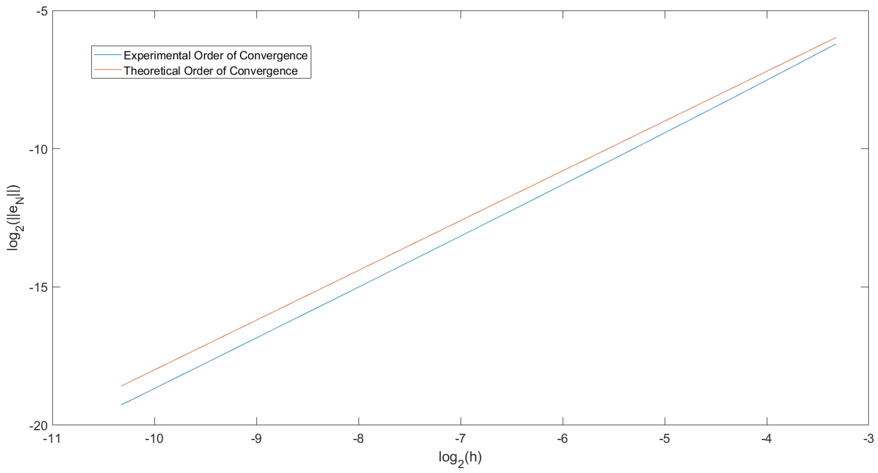
In Figure 1, we have plotted the order of convergence for Example 1. From Equation (51), we have for ,
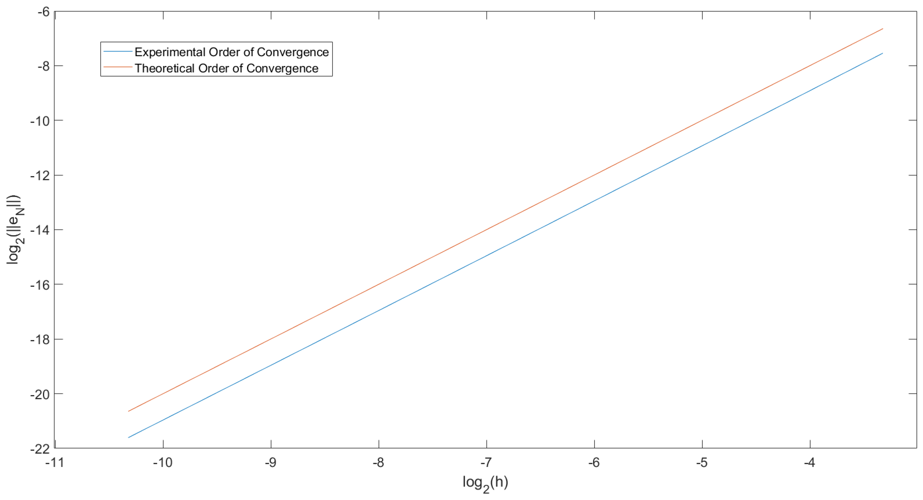
We can now plot this graph such that and let and . Doing this, we get that the gradient of the graph would equal the EOC. To compare this to the theoretical order of convergence, we have also plotted the straight line . For Figure 1, we use . We can observe that the two lines drawn are parallel. Therefore, we can conclude that the order of convergence of this predictor–corrector method is for when . A similar result can be obtained for when . Figure 2 shows the same graph but for . However, now we can see that the line is parallel to the straight line , which is what we expected as the convergence order should tend to 2 for .
Example 2
(y is smooth). Consider the following nonlinear fractional differential equation, with ,
where,
The exact solution of this equation is,
In Table 3, Table 4 and Table 5, we can see the maximum absolute error and experimental order of convergence (EOC) for the predictor–corrector method at varying and N values. For our different , we have chosen N values as . As we can apply Theorems 6 and 7 and more specifically, Corollary 2. As we can see, the EOCs for the above example verifies these theorems. When , we find that the EOC is close to and when , we find that the EOC is close to . Finally, when , we have that the EOC is close to .
Example 3
(f is smooth). Consider the following nonlinear fractional differential equation, with ,
The exact solution of this equation is . Therefore, , where is defined as the Mittag–Leffler function,
Therefore, f is smooth. As such, this equation fulfils the conditions of Theorem 8. In Table 6 and Table 7, we can see the maximum absolute error and experimental order of convergence (EOC) for the predictor–corrector method at varying and N values. For our different , we have chosen N values as . As f is sufficiently smooth, we can apply Theorem 8. As we can see, the EOCs for the above example verifies these theorems. When , we have that the EOC is close to . For , we have the EOC is close to 2.
5. Conclusions
In this paper, we proposed a predictor–corrector method for solving Caputo–Hadamard fractional differential equations. Both the initial data f and the unknown solution y were investigated to see how the different smoothness conditions affected the convergence order. It was found under optimal conditions and with that we can obtain a theoretical convergence order of 2. However, under certain smoothness conditions, a suboptimal convergence order is achieved, often depending on the fractional part of . Several numerical simulations are given to support the theoretical results obtained above in terms of the error estimates.
Author Contributions
We contributed equally to this work. C.W.H.G. considered the theoretical analysis, performed the numerical simulation, and wrote the original version of the work. Y.Y. introduced and guided this research topic. All authors have read and agreed to the published version of the manuscript.
Funding
This research received no external funding.
Conflicts of Interest
The authors declare no conflict of interest.
References
- Diethelm, K. The Analysis of Fractional Differential Equations; Lecture Notes in Mathematics; Springer: Berlin/Heidelberg, Germany, 2010. [Google Scholar]
- Kilbas, A.A.; Srivastava, H.M.; Trujillo, J.J. Theory and Applications of Fractional Differential Equations; North-Holland Mathematics Studies; Elsevier: Amsterdam, The Netherlands, 2006; Volume 204. [Google Scholar]
- Oldman, B.K.; Spanier, J. The Fractional Calculus; Academic Press: New York, NY, USA, 1974. [Google Scholar]
- Podlubny, I. Fractional Differential Equations; Math, Science and Engineering; Academic Press: San Diego, CA, USA, 1999. [Google Scholar]
- Adjabi, Y.; Jarad, F.; Baleanu, D.; Abdeljawad, T. On Cauchy problems with Caputo Hadamard fractional derivatives. J. Comput. Anal. Appl. 2016, 21, 661–681. [Google Scholar]
- Garra, R.; Mainardi, F.; Spada, G. A generalization of the Lomnitz logarithmic creep law via Hadamard fractional calculus. Chaos Solitons Fractals 2017, 102, 333–338. [Google Scholar] [CrossRef]
- Gohar, M.; Li, C.; Yin, C. On Caputo Hadamard fractional differential equations. Int. J. Comput. Math. 2020, 97, 1459–1483. [Google Scholar] [CrossRef]
- Jarad, F.; Abdeljawad, T.; Baleanu, D. Caputo-type modification of the Hadamard fractional derivatives. Adv. Differ. Equ. 2012, 2012, 142. [Google Scholar] [CrossRef]
- Kilbas, A.A. Hadamard-type fractional calculus. J. Korean Math. Soc. 2001, 38, 1191–1204. [Google Scholar]
- Li, C.; Cai, M. Theory and Numerical Approximations of Fractional Integrals and Derivatives; SIAM: Philadelphia, PA, USA, 2019. [Google Scholar]
- Ma, L. On the kinetics of Hadamard-type fractional differential systems. Fract. Calc. Appl. Anal. 2020, 23, 553–570. [Google Scholar] [CrossRef]
- Hadamard, J. Essai sur létude des fonctions donnes par leur developpment de Taylor. J. Pure Appl. Math. 1892, 4, 101–186. [Google Scholar]
- Gohar, M.; Li, C.; Li, Z. Finite Difference Methods for Caputo-Hadamard Fractional Differential Equations. Mediterr. J. Math. 2020, 17, 194. [Google Scholar] [CrossRef]
- Green, C.W.H.; Liu, Y.; Yan, Y. Numerical methods for Caputo- Hadamard fractional differential equations with graded and non-uniform meshes. Mathematics 2021, 9, 2728. [Google Scholar] [CrossRef]
- Diethelm, K.; Ford, N.J.; Freed, A.D. Detailed error analysis for a fractional Adams method. Numer. Algorithms 2004, 36, 31–52. [Google Scholar] [CrossRef]
- Liu, Y.; Roberts, J.; Yan, Y. Detailed error analysis for a fractional Adams method with graded meshes. Numer. Algorithms 2018, 78, 1195–1216. [Google Scholar] [CrossRef]
- Li, C.; Li, Z.; Wang, Z. Mathematical analysis and the local discontinuous Galerkin method for Caputo-Hadamard fractional partial differential equation. J. Sci. Comput. 2020, 85, 41. [Google Scholar] [CrossRef]
- Zhang, Y.; Sun, Z.; Liao, H. Finite difference methods for the time fractional diffusion equation on non-uniform meshes. Int. J. Comput. Math. 2014, 265, 195–210. [Google Scholar] [CrossRef]
- Li, C.; Yi, Q.; Chen, A. Finite difference methods with non-uniform meshes for nonlinear fractional differential equations. J. Comput. Phys. 2016, 316, 614–631. [Google Scholar] [CrossRef]
- Diethelm, K. Generalized compound quadrature formulae for finite-part integrals. IMA J. Numer. Anal. 1997, 17, 479–493. [Google Scholar] [CrossRef]
- Zabidi, N.A.; Majid, Z.A.; Kilicman, A. Numerical solution of fractional differential equations with Caputo derivative by using numerical fractional predict-correct technique. Adv. Contin. Discret. Model. 2022, 2022, 26. [Google Scholar] [CrossRef]
- Ahmad, B.; Alsaedi, A.; Ntouyas, S.K.; Tariboon, J. Hadamard-Type Fractional Differential Equations, Inclusions and Inequalities; Springer: Cham, Switzerland, 2017. [Google Scholar]
- Wang, G.; Ren, X.; Zhang, L.; Ahmad, B. Explicit iteration and unique positive solution for a Caputo-Hadamard fractional turbulent flow model. IEEE Access 2019, 7, 109833–109839. [Google Scholar] [CrossRef]
- Awadalla, M.; Yameni, Y.Y.; Abuassba, K. A new fractional model for the cancer treatment by radiotherapy using the Hadamard fractional derivative. OMJ 1971, 1, 14–18. [Google Scholar]
- Diethelm, K.; Ford, N.J. Analysis of fractional differential equations. J. Math. Anal. Appl. 2002, 265, 229–248. [Google Scholar] [CrossRef]
- Miller, R.K.; Feldstein, A. Smoothness of solutions of Volterra integral equations with weakly singular kernels. SIAM J. Math. Anal. 1971, 2, 242–258. [Google Scholar] [CrossRef] [Green Version]
Figure 1.
Graph showing the experimental order of convergence (EOC) at T = 2 in Example 1 with .

Figure 2.
Graph showing the experimental order of convergence (EOC) at T = 2 in Example 1 with .


Table 1.
Table showing the maximum absolute error and EOC for solving (47) using the predictor–corrector method for .
Table 1.
Table showing the maximum absolute error and EOC for solving (47) using the predictor–corrector method for .
| N | EOC | EOC | EOC | |||
|---|---|---|---|---|---|---|
| 10 | 6.839 × 10 | 2.607 × 10 | 1.350 × 10 | |||
| 20 | 2.064 × 10 | 1.728 | 7.433 × 10 | 1.810 | 3.542 × 10 | 1.930 |
| 40 | 6.576 × 10 | 1.650 | 2.209 × 10 | 1.751 | 9.534 × 10 | 1.894 |
| 80 | 2.193 × 10 | 1.584 | 6.768 × 10 | 1.706 | 2.610 × 10 | 1.869 |
| 160 | 7.561 × 10 | 1.536 | 2.120 × 10 | 1.675 | 7.225 × 10 | 1.853 |
| 320 | 2.671 × 10 | 1.502 | 6.744 × 10 | 1.653 | 2.015 × 10 | 1.842 |
| 640 | 9.600 × 10 | 1.476 | 2.169 × 10 | 1.637 | 5.652 × 10 | 1.834 |
| 1280 | 3.497 × 10 | 1.457 | 7.026 × 10 | 1.626 | 1.591 × 10 | 1.829 |
Table 2.
Table showing the maximum absolute error and EOC for solving (47) using the predictor–corrector method for .
Table 2.
Table showing the maximum absolute error and EOC for solving (47) using the predictor–corrector method for .
| N | EOC | EOC | EOC | |||
|---|---|---|---|---|---|---|
| 10 | 6.166 × 10 | 5.475 × 10 | 5.369 × 10 | |||
| 20 | 1.463 × 10 | 2.076 | 1.319 × 10 | 2.053 | 1.319 × 10 | 2.026 |
| 40 | 3.497 × 10 | 2.065 | 3.207 × 10 | 2.040 | 3.259 × 10 | 2.017 |
| 80 | 8.408 × 10 | 2.056 | 7.853 × 10 | 2.030 | 8.091 × 10 | 2.010 |
| 160 | 2.033 × 10 | 2.049 | 1.934 × 10 | 2.022 | 2.014 × 10 | 2.006 |
| 320 | 4.935 × 10 | 2.042 | 4.783 × 10 | 2.016 | 5.022 × 10 | 2.004 |
| 640 | 1.203 × 10 | 2.036 | 1.187 × 10 | 2.011 | 1.253 × 10 | 2.002 |
| 1280 | 2.943 × 10 | 2.031 | 2.951 × 10 | 2.008 | 3.131 × 10 | 2.001 |
Table 3.
Table showing the maximum absolute error and EOC for solving (53) using the predictor–corrector method for .
Table 3.
Table showing the maximum absolute error and EOC for solving (53) using the predictor–corrector method for .
| N | EOC | EOC | EOC | |||
|---|---|---|---|---|---|---|
| 10 | 2.225 × 10 | 9.375 × 10 | 5.123 × 10 | |||
| 20 | 1.261 × 10 | 0.819 | 3.345 × 10 | 1.487 | 1.622 × 10 | 1.660 |
| 40 | 5.625 × 10 | 1.164 | 1.196 × 10 | 1.484 | 5.255 × 10 | 1.626 |
| 80 | 2.387 × 10 | 1.237 | 4.343 × 10 | 1.461 | 1.739 × 10 | 1.595 |
| 160 | 1.004 × 10 | 1.249 | 1.606 × 10 | 1.436 | 5.856 × 10 | 1.571 |
| 320 | 4.242 × 10 | 1.243 | 6.033 × 10 | 1.412 | 1.998 × 10 | 1.552 |
| 640 | 1.805 × 10 | 1.233 | 2.299 × 10 | 1.392 | 6.884 × 10 | 1.537 |
| 1280 | 7.742 × 10 | 1.221 | 8.864 × 10 | 1.375 | 2.389 × 10 | 1.527 |
Table 4.
Table showing the maximum absolute error and EOC for solving (53) using the predictor–corrector method for .
Table 4.
Table showing the maximum absolute error and EOC for solving (53) using the predictor–corrector method for .
| N | EOC | EOC | ||
|---|---|---|---|---|
| 10 | 5.507 × 10 | 1.162 × 10 | ||
| 20 | 1.931 × 10 | 1.512 | 5.100 × 10 | 1.188 |
| 40 | 7.031 × 10 | 1.457 | 2.300 × 10 | 1.151 |
| 80 | 2.635 × 10 | 1.416 | 1.051 × 10 | 1.129 |
| 160 | 1.008 × 10 | 1.386 | 4.847 × 10 | 1.116 |
| 320 | 3.920 × 10 | 1.363 | 2.247 × 10 | 1.109 |
| 640 | 1.541 × 10 | 1.347 | 1.045 × 10 | 1.105 |
| 1280 | 6.110 × 10 | 1.335 | 4.863 × 10 | 1.103 |
Table 5.
Table showing the maximum absolute error and EOC for solving (53) using the predictor–corrector method for .
Table 5.
Table showing the maximum absolute error and EOC for solving (53) using the predictor–corrector method for .
| N | EOC | EOC | EOC | |||
|---|---|---|---|---|---|---|
| 10 | 6.166 × 10 | 5.475 × 10 | 5.369 × 10 | |||
| 20 | 1.463 × 10 | 2.076 | 1.319 × 10 | 2.053 | 1.319 × 10 | 2.026 |
| 40 | 3.497 × 10 | 2.065 | 3.207 × 10 | 2.040 | 3.259 × 10 | 2.017 |
| 80 | 8.408 × 10 | 2.056 | 7.853 × 10 | 2.030 | 8.091 × 10 | 2.010 |
| 160 | 2.033 × 10 | 2.049 | 1.934 × 10 | 2.022 | 2.014 × 10 | 2.006 |
| 320 | 4.935 × 10 | 2.042 | 4.783 × 10 | 2.016 | 5.022 × 10 | 2.004 |
| 640 | 1.203 × 10 | 2.036 | 1.187 × 10 | 2.011 | 1.253 × 10 | 2.002 |
| 1280 | 2.943 × 10 | 2.031 | 2.951 × 10 | 2.008 | 3.131 × 10 | 2.001 |
Table 6.
Table showing the maximum absolute error and EOC for solving Example 3 using the predictor–corrector method for .
Table 6.
Table showing the maximum absolute error and EOC for solving Example 3 using the predictor–corrector method for .
| N | EOC | EOC | EOC | |||
|---|---|---|---|---|---|---|
| 10 | 1.353 × 10 | 6.520 × 10 | 3.414 × 10 | |||
| 20 | 4.324 × 10 | 1.646 | 1.937 × 10 | 1.751 | 8.704 × 10 | 1.972 |
| 40 | 1.466 × 10 | 1.560 | 6.019 × 10 | 1.686 | 2.270 × 10 | 1.939 |
| 80 | 5.159 × 10 | 1.507 | 1.919 × 10 | 1.649 | 5.990 × 10 | 1.922 |
| 160 | 1.863 × 10 | 1.470 | 6.211 × 10 | 1.628 | 1.591 × 10 | 1.913 |
| 320 | 6.863 × 10 | 1.441 | 2.027 × 10 | 1.615 | 4.239 × 10 | 1.908 |
| 640 | 2.570 × 10 | 1.417 | 6.652 × 10 | 1.608 | 1.132 × 10 | 1.905 |
| 1280 | 9.752 × 10 | 1.398 | 2.189 × 10 | 1.604 | 3.026 × 10 | 1.904 |
Table 7.
Table showing the maximum absolute error and EOC for solving Example 3 using the predictor–corrector method for .
Table 7.
Table showing the maximum absolute error and EOC for solving Example 3 using the predictor–corrector method for .
| N | EOC | EOC | EOC | |||
|---|---|---|---|---|---|---|
| 10 | 2.457 × 10 | 2.108 × 10 | 1.507 × 10 | |||
| 20 | 5.847 × 10 | 2.071 | 5.141 × 10 | 2.036 | 3.723 × 10 | 2.017 |
| 40 | 1.400 × 10 | 2.062 | 1.261 × 10 | 2.027 | 9.236 × 10 | 2.011 |
| 80 | 3.374 × 10 | 2.053 | 3.109 × 10 | 2.020 | 2.298 × 10 | 2.007 |
| 160 | 8.213 × 10 | 2.039 | 7.693 × 10 | 2.015 | 5.728 × 10 | 2.004 |
| 320 | 2.016 × 10 | 2.027 | 1.909 × 10 | 2.011 | 1.430 × 10 | 2.003 |
| 640 | 4.975 × 10 | 2.019 | 4.748 × 10 | 2.008 | 3.570 × 10 | 2.002 |
| 1280 | 1.233 × 10 | 2.013 | 1.183 × 10 | 2.005 | 8.919 × 10 | 2.001 |
Publisher’s Note: MDPI stays neutral with regard to jurisdictional claims in published maps and institutional affiliations. |
© 2022 by the authors. Licensee MDPI, Basel, Switzerland. This article is an open access article distributed under the terms and conditions of the Creative Commons Attribution (CC BY) license (https://creativecommons.org/licenses/by/4.0/).
Share and Cite
MDPI and ACS Style
Green, C.W.H.; Yan, Y. Detailed Error Analysis for a Fractional Adams Method on Caputo–Hadamard Fractional Differential Equations. Foundations 2022, 2, 839-861. https://0-doi-org.brum.beds.ac.uk/10.3390/foundations2040057
AMA Style
Green CWH, Yan Y. Detailed Error Analysis for a Fractional Adams Method on Caputo–Hadamard Fractional Differential Equations. Foundations. 2022; 2(4):839-861. https://0-doi-org.brum.beds.ac.uk/10.3390/foundations2040057
Chicago/Turabian StyleGreen, Charles Wing Ho, and Yubin Yan. 2022. "Detailed Error Analysis for a Fractional Adams Method on Caputo–Hadamard Fractional Differential Equations" Foundations 2, no. 4: 839-861. https://0-doi-org.brum.beds.ac.uk/10.3390/foundations2040057