
Exploratory Analysis of Distributional Data Using the Quantile Method
School of Science and Engineering, Tokyo Denki University, Hatoyama, Saitama 350-0394, Japan
AppliedMath 2024, 4(1), 261-288; https://0-doi-org.brum.beds.ac.uk/10.3390/appliedmath4010014
Submission received: 23 October 2023
/
Revised: 2 January 2024
/
Accepted: 26 January 2024
/
Published: 17 February 2024
Abstract
:The quantile method transforms each complex object described by different histogram values to a common number of quantile vectors. This paper retraces the authors’ research, including a principal component analysis, unsupervised feature selection using hierarchical conceptual clustering, and lookup table regression model. The purpose is to show that this research is essentially based on the monotone property of quantile vectors and works cooperatively in the exploratory analysis of the given distributional data.
1. Introduction
The extension of various statistical methods has been developed for complex data types, including histogram-valued symbolic data [1,2,3,4]. This paper considers the following three research categories.
1.1. Principal Component Analysis (PCA)
The main purpose of traditional PCA is to transform a number of possibly correlated variables into a small number of uncorrelated variables, which are called principal components. In the generalization of PCA for complex data types, mainstream research uses Pearson’s approach. For example, a summary of various generalized PCA for interval data are given in [5]. The authors proposed a general method of PCA based on the quantification method using generalized Minkowski metrics [6,7] and proposed the quantile method of PCA for general distributional data [8,9].
1.2. Clustering and Unsupervised Feature Selection
In the generalization of hierarchical clustering for histogram-valued data, the main problem is how to define an appropriate similarity or dissimilarity measure for the given objects and/or clusters. A hierarchical clustering method based on the Wasserstein distance [10] and a nonhierarchical method based on the dynamical clustering method [11] are typical examples. The authors also proposed a hierarchical conceptual clustering method based on the quantile method [12].
In unsupervised feature selection, clustering is a useful tool for searching for informative feature subsets. By combining existing clustering methods with an appropriate wrapper method, for example, we can achieve unsupervised feature selection. The authors proposed an unsupervised feature selection method for general distributional data using hierarchical conceptual clustering based on compactness [13]. Compactness plays multiple roles, i.e., the measures of similarity between objects and/or clusters, cluster quality, and feature effectiveness. This property greatly simplifies the task of feature selection.
1.3. Regression Models
The extension of linear regression models for histogram-valued variables was developed in [14,15,16,17,18,19,20]. In these studies, some functional forms between the response variable and the explanatory variable(s) have been proposed under the appropriately defined optimality criterion. As another very different method, the authors proposed the lookup table regression model (LTRM) for histogram data using the quantile method [21,22].
This paper retraces the aforementioned studies based on the quantile method and describes the proposed methods working cooperatively in an exploratory analysis of the given distributional data.
Section 2 describes the representation of objects by quantile vectors and bin rectangles. Section 2.1, Section 2.2 and Section 2.3 describe the quantile method, which transforms each object with p distributional feature variables into a description using a series of m + 1 p-dimensional quantile vectors. It further describes these objects using a series of m p-dimensional bin rectangles, each spanned by adjacent quantile vectors, where m is predetermined integer. Section 2.4 and Section 2.5 define the concept size of bin rectangles and the concept size of the Cartesian join of objects. The Cartesian join generates a generalized concept for the two given objects. Section 2.6 defines the measure of compactness for the two given objects and/or clusters under the assumption of equal bin probabilities. Compactness plays the central role in our unsupervised feature selection using hierarchical conceptual clustering.
Section 3 discusses the results of an exploratory analysis of two distributional datasets: oil data and hardwood data. Section 3.1 summarizes the quantile method of PCA and dual-PCA using rank order correlation coefficients under the monotone property of quantile vectors. Section 3.2 describes the unsupervised feature selection method using the hierarchical conceptual clustering based on compactness.
Section 3.3 proposes the lookup table regression model (LTRM) for distributional data based on monotone blocks segmentation (MBS).
Section 4 includes a concluding summary.
2. Quantile Vectors, Bin Rectangles, and Compactness
Let U = {ωi, i = 1, 2, …, N} be the set of given objects, and let feature variables Fj, j = 1, 2, …, p describe each object. Let Dj be the domain of feature Fj, j = 1, 2, …, p. Then, the feature space is defined by the following:
D(p) = D1 × D2 × ··· × Dp.
Each element of D(p) is represented by:
where Ej is the feature value of Fj, j = 1, 2, …, p.
E = E1 × E2 × ··· × Ep,
2.1. Histogram-Valued Feature
For each object ωi, let each feature Fj be represented by a histogram value as follows:
where pij1 + pij2 + ··· + pijnij = 1 and nij is the number of bins that compose the histogram Eij. Therefore, the Cartesian product of p histogram values represents the object ωi:
Eij = {[aijk, aij(k+1)), pijk; k = 1, 2, …, nij},
Ei = Ei1 × Ei2 × ··· × Eip.
Because the interval-valued feature is a special case of a histogram feature with nij = 1 and pij1 = 1, the representation of (3) is reduced to an interval, as follows:
Eij = [aij1, aij2).
2.2. Representation of Histograms by Common Number of Quantiles
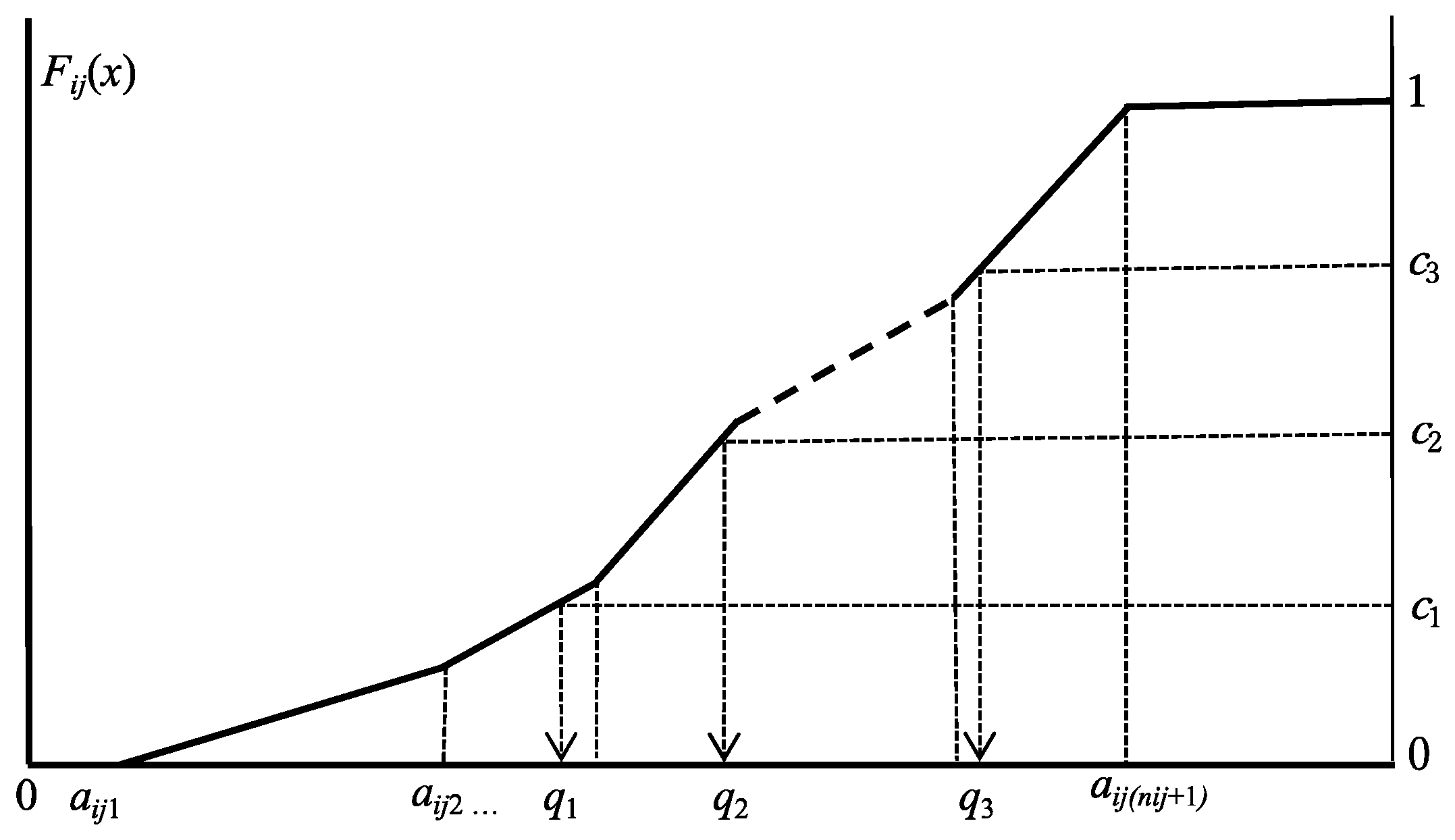
Let ωi ∈ U be the given object, and let Eij be a histogram value in (3) for a feature Fj. Then, under the assumption that nij bins have uniform distributions, we define the cumulative distribution function Fij(x) of the histogram (3) as follows:
Fij(x) = 0 for x ≤ aij1
Fij(x) = pij1(x − aij1)/(aij2 − aij1) for aij1 ≤ x < aij2
Fij(x) = F(aij1) + pij2(x − aij2)/(aij3 − aij2) for aij2 ≤ x < aij3
······
Fij(x) = F(aij(nij−1)) + pijnij(x − aijnij)/(aij(nij+1) − aijnij) for aijnij ≤ x < aij(nij+1)
Fij(x) = 1 for aij(nij+1) ≤ x.
Figure 1 illustrates a cumulative distribution function for a histogram feature value, where c1, c2, and c3 are cut points for the case m = 4, and q1, q2, and q3 are the corresponding quantile values.
Our general procedure to have common representation for histogram-valued data is as follows.
- (1)
- We choose a common number m of quantiles.
- (2)
- Let c1, c2, …, cm−1 be preselected cut points dividing the range of the distribution function Fij(x) into continuous intervals, i.e., bins with preselected probabilities associated with m − 1 cut points.
- (3)
- For the given cut points c1, c2, …, cm−1, we calculate the corresponding quantiles by solving the following equations:
Fij(xij0) = 0, (i.e., xij0 = aij1)
Fij(xij1) = c1, Fij(xij2) = c2, …, Fij(xij(m−1)) = cm−1, and
Fij(xijm) = 1, (i.e., xijm = aij(nij+1)).
Fij(xij1) = c1, Fij(xij2) = c2, …, Fij(xij(m−1)) = cm−1, and
Fij(xijm) = 1, (i.e., xijm = aij(nij+1)).
Therefore, we describe each object ωi ∈ U for each feature Fj using a (m + 1) tuple:
and the corresponding histogram using:
where we assume that c0 = 0 and cm = 1. In (7), (ck+1 − ck), k = 0, 1, …, m − 1, denote bin probabilities using the preselected cut point probabilities c1, c2, …, cm−1. In the quartile case, m = 4 and c1 = 1/4, c2 = 2/4, and c3 = 3/4, four bins, [xij0, xij1), [xij1, xij2), [xij2, xij3), and [xij3, xij4), have the same bin probability: 1/4.
(xij0, xij1, xij2, …, xij(m−1), xijm), j = 1, 2, …, p
Eij = {[xijk, xij(k+1)), (ck+1 − ck); k = 0, 1, …, m − 1}, j = 1, 2, …, p,
The number of bins of the given histograms may be mutually different in general. However, we can obtain (m + 1)-tuples as the common representation for all histograms by selecting an integer m and a set of cut points.
2.3. Quantile Vectors and Bin Rectangles
For each object ωi ∈ U, we define (m + 1) p-dimensional numerical vectors, which are called the quantile vectors, as follows.
xik = (xi1k, xi2k, …, xipk), k = 0, 1, …, m.
We call xi0 and xim the minimum quantile vector and the maximum quantile vector, respectively. Therefore, m + 1 quantile vectors {xi0, xi1, …, xim} in Rp describe each object ωi ∈ U together with cut point probabilities.
The components of m + 1 quantile vectors in (8) for object ωi ∈ U satisfy the inequalities:
xij0 ≤ xij1 ≤ xij2 ≤ ··· ≤ xij(m−1) ≤ xijm, j = 1, 2, …, p.
Therefore, m + 1 quantile vectors in (8) for object ωi ∈ U satisfy the monotone property:
xi0 ≤ xi1 ≤ ··· ≤ xim.
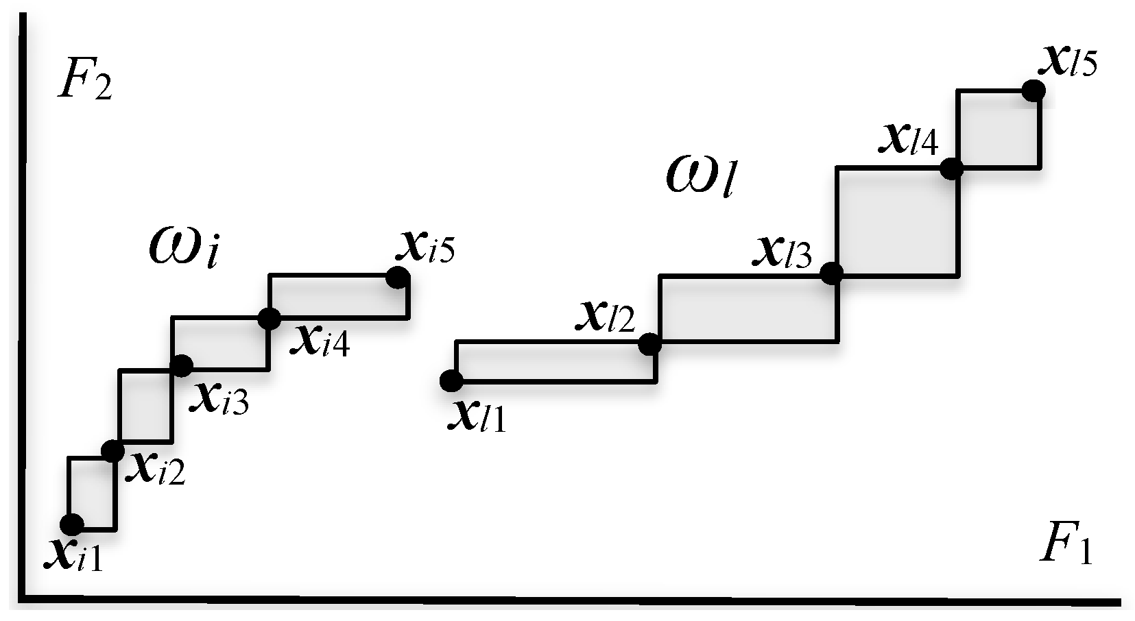
For the series of quantile vectors xi0, xi1, …, xim of object ωi ∈ U, we define m series of p dimensional rectangles, which are called bin rectangles, spanned by adjacent quantile vectors xik and xi(k+1), k = 0, 1, …, m − 1, as follows:
where xik⊞xi(k+1) is the Cartesian join [6, 7] of xik and xi(k+1) obtained using the Cartesian join xijk⊞xij(k+1) = [xijk, xij(k+1)], j = 1, 2, …, p.
B(xik, xi(k+1)) = xik⊞xi(k+1) = [xi1k⊞xi1(k+1)] × [xi2k⊞xi2(k+1)] × ··· × [xipk⊞xip(k+1)]
= [xi1k, xi1(k+1)] × [xi2k, xi2(k+1)] × ··· × [xipk, xip(k+1)], k = 0, 1, …, m − 1,
= [xi1k, xi1(k+1)] × [xi2k, xi2(k+1)] × ··· × [xipk, xip(k+1)], k = 0, 1, …, m − 1,
Figure 2 illustrates two objects using two-dimensional bin rectangles in the quartile case. Because a bin rectangle is regarded as a conjunctive logical expression, we also use the term concept. Therefore, four bin rectangles describe each of these objects ωi and ωl as a concept.
2.4. Concept Size of Bin Rectangles
For each feature Fj, j = 1, 2, …, p, let the domain Dj of feature values be the following interval:
where
Dj = [xjmin, xjmax], j = 1, 2, …, p,
xjmin = min(x1j0, x2j0, …, xNj0) and xjmax = max(x1jm, x2jm, …, xNjm).
Definition 1.
Let object ωi ∈ U be described using the set of histograms for Eij in (7). We define the average concept size P(Eij) of m bins for histogram Eij as follows:
P(Eij) = {c1(xij1 − xij0) + (c2 − c1)(xij2 − xij1) + ··· + (ck − c(k−1))(xijk − xij(k−1)) + ···
+ (cm−1 − cm−2)(xij(m−1) − xij(m−2)) + (1 − cm−1)(xijm − xij(m−1))}/|Dj|.
+ (cm−1 − cm−2)(xij(m−1) − xij(m−2)) + (1 − cm−1)(xijm − xij(m−1))}/|Dj|.
The average concept size P(Eij) satisfies the inequality:
0 ≤ P(Eij) ≤ 1, j = 1, 2, …, p.
Proposition 1.
- (1)
- When m bin probabilities are the same, the average concept size of m bins is reduced to the form:
P(Eij) = (xijm − xij0)/(m|Dj|), j = 1, 2, …, p.
- (2)
- When m bin widths are the same size wij, we have:
P(Eij) = wij/|Dj|, j = 1, 2, …, p.
- (3)
- It is clear that:
wij = (xijm − xij0)/m.
This proposition asserts that both extremes yield the same conclusion.
Definition 2.
Let Ei = Ei1 × Ei2 × ··· × Eip be the description of p histograms in Rp for ωi ∈ U. Then, we define the concept size P(Ei) of Ei using the arithmetic mean:
P(Ei) = (P(Ei1) + P(Ei2) + ··· + P(Eip))/p.
From (13), It is clear that:
0 ≤ P(Ei) ≤ 1.
Definition 3.
Let P(B(xik, xi(k+1))), k = 0, 1, …, m − 1, be the concept size of m bin rectangles defined by the average of p normalized bin widths:
P(B(xik, xi(k+1))) = {|xi1(k+1) − xi1k|/|D1| + |xi2(k+1) − xi2k|/|D2| + ··· + |xip(k+1) − xipk|/|Dp|}/p, k = 0, 1, …, m − 1.
Then (12) and (19) lead to the following proposition.
Proposition 2.
The concept size P(Ei) is equivalent to the average value of m concept sizes of bin rectangles:
where c0 = 0 and cm = 1.
P(Ei) = (c1 − c0)P(B(xi0, xi1)) + (c2 − c1)P(B(xi1, xi2)) + ··· + (cm − c(m−1))P(B(xi(m−1), xim)),
In Figure 2, two objects, ωi and ωl, are represented by four bin rectangles with the same probability: 1/4. According to Proposition 2, object ωi has a smaller concept size than object ωl.
2.5. Concept Size of the Cartesian Join of Objects
Let Eij and Elj be two histogram values of objects ωi, ωl ∈ U with respect to the j-th feature. We represent a generalized histogram value of Eij and Elj, which is called the Cartesian join of Eij and Elj, using Eij⊞Elj. Let FEij(x) and FElj(x) be the cumulative distribution functions associated with histograms Eij and Elj, respectively.
Definition 4.
We define the cumulative distribution function for the Cartesian join Eij⊞Elj as follows:
FEij⊞Elj(x) = (FEij(x) + FElj(x))/2, j = 1, 2, …, p.
Then, by applying the same integer m and the set of cut point probabilities, c1, c2, …, cm−1, used for Eij and Elj, we define the histogram of the Cartesian join Eij⊞Elj for the j-th feature as:
where we assume that c0 = 0 and cm = 1 and that the suffix (i + l) denotes the quantile values for the Cartesian join Eij⊞Elj. We should note that x(i+l)j0 = min(xij0, xlj0) and x(i+l)jm = max(xijm, xljm).
Eij⊞Elj = {[x(i+l)jk, x(i+l)j(k+1)), (ck+1 − ck); k = 0, 1, …, m − 1}, j = 1, 2, …, p,
Definition 5.
We define the average concept size P(Eij⊞Elj) of m bins for the Cartesian join Eij and Elj under the j-th feature as follows:
P(Eij⊞Elj) = {c1(x(i+l)j1 − x(i+l)j0) + (c2 − c1)(x(i+l)j2 − x(i+l)j1) + ···
+ (cm−1 − cm−2)(x(i+l)j(m−1) − x(i+l)j(m−2)) + (1 − cm−1)(x(i+l)jm − x(i+l)j(m−1))}/|Dj|
= {c1|x(i+l)j0⊞x(i+l)j1| + (c2 − c1)|x(i+l)j1⊞x(i+l)j2| + ···
+ (cm−1 − cm−2)|x(i+l)j(m−2)⊞x(i+l)j(m−1)| + (1 − cm−1)|x(i+l)j(m−1)⊞x(i+l)jm|}/|Dj|, j = 1, 2, …, p.
+ (cm−1 − cm−2)(x(i+l)j(m−1) − x(i+l)j(m−2)) + (1 − cm−1)(x(i+l)jm − x(i+l)j(m−1))}/|Dj|
= {c1|x(i+l)j0⊞x(i+l)j1| + (c2 − c1)|x(i+l)j1⊞x(i+l)j2| + ···
+ (cm−1 − cm−2)|x(i+l)j(m−2)⊞x(i+l)j(m−1)| + (1 − cm−1)|x(i+l)j(m−1)⊞x(i+l)jm|}/|Dj|, j = 1, 2, …, p.
The average concept size satisfies the inequality:
0 ≤ P(Eij⊞Elj) ≤ 1, j = 1, 2, …, p.
Proposition 3.
When m bin probabilities are the same or m bin widths are the same, we have the following monotone property:
P(Eij), P(Elj) ≤ P(Eij⊞Elj), j = 1, 2, …, p.
Definition 6.
Let Ei = Ei1 × Ei2 × ··· × Eip and El = El1 × El2 × ··· × Elp be the descriptions of p histograms in Rp for ωi and ωl, respectively. Then, we define the concept size P(Ei⊞El) for the Cartesian join of Ei and El using the arithmetic mean, as follows:
P(Ei⊞El) = (P(Ei1⊞El1) + P(Ei2⊞El2) + ··· + P(Eip⊞Elp))/p.
From (24), it is clear that:
0 ≤ P(Ei⊞El) ≤ 1.
Definition 7.
Let x(i+l)k, k = 0, 1, …, m be the quantile vectors for the Cartesian join Ei⊞El, and let P(B(x(i+l)k, x(i+l)(k+1))), k = 0, 1, …, m − 1 be the concept sizes of m bin rectangles defined by the average of p normalized bin widths, as follows:
P(B(xik, xi(k+1))) = {|xi1k⊞xi1(k+1)|/|D1| + |xi2k⊞xi2(k+1)|/|D2| + ··· + |xipk⊞xip(k+1)|/|Dp|}/p, k = 0, 1, …, m − 1.
Then, we have the following result:
Proposition 4.
The concept size P(Ei⊞El) is equivalent to the average value of m concept sizes of bin rectangles:
where c0 = 0 and cm = 1.
P(Ei⊞El) = (c1 − c0)P(B(x(i+l)0, x(i+l)1)) + (c2 − c1)P(B(x(i+l)1, x(i+l)2)) + ··· + (cm − c(m−1))P(B(x(i+l)(m−1), x(i+l)m)),
We have the following monotone property from Proposition 3 and Definition 6.
Proposition 5.
When m bin probabilities are the same or m bin widths are the same for all features, we have the monotone property:
P(Ei), P(El) ≤ P(Ei⊞El).
This property plays a very important role in our hierarchical conceptual clustering in Section 3.2.
2.6. Compactness and Its Properties
In the following section, we assume that the given distributional data have the same representation using m quantile values with the same bin probabilities.
Definition 8.
Under the assumption of equal bin probabilities, we define the compactness of the generalized concept of ωi and ωl as follows:
C(ωi, ωl) = P(Ei⊞El) = (P(B(x(i+l)0, x(i+l)1)) + P(B(x(i+l)1, x(i+l)2)) + ··· + P(B(x(i+l)(m−1), x(i+l)m))/m.
The compactness satisfies the following properties:
Proposition 6.
- (1)
- 0 ≤ C(ωi, ωl) ≤ 1, normalization.
- (2)
- C(ωi, ωl) = 0 iff Ei ≡ El and has null size (P(Ei) = 0).
- (3)
- C(ωi, ωi), C(ωl, ωl) ≤ C(ωi, ωl), monotone property.
- (4)
- C(ωi, ωl) = C(ωl, ωi), symmetric property.
- (5)
- C(ωi, ωr) ≤ C(ωi, ωl) + C(ωl, ωr) may not hold in general.
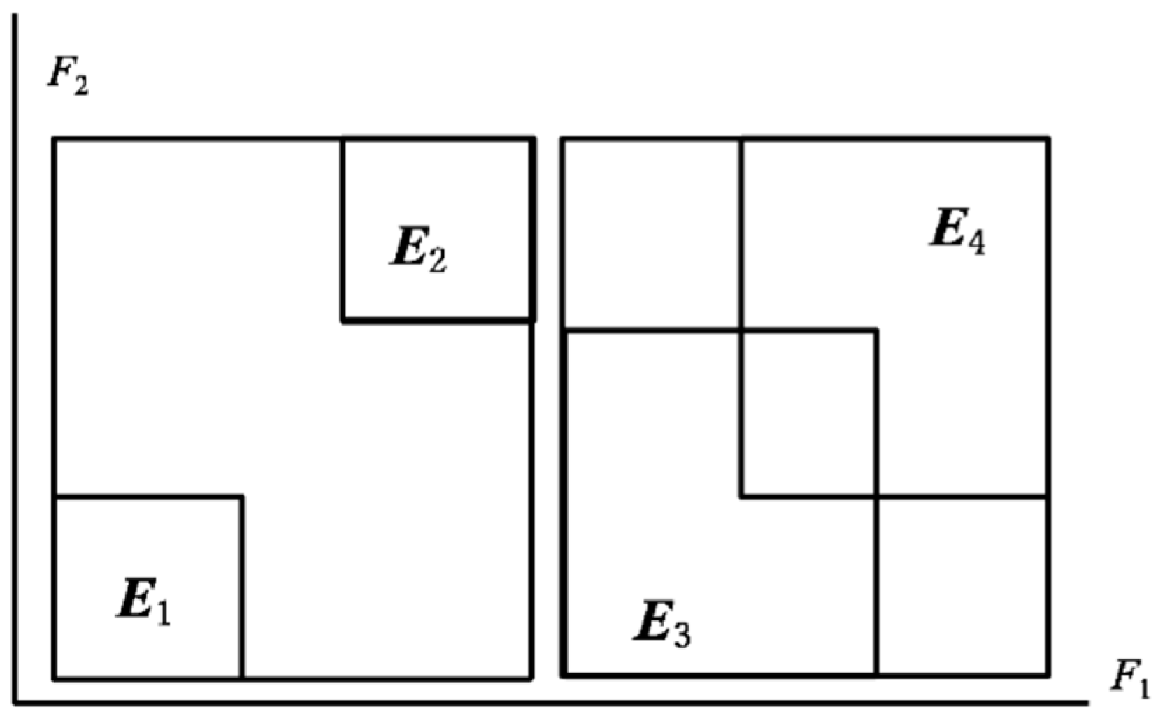
Figure 3 illustrates the Cartesian join for interval-valued objects. We should note that the compactness, C(ω1, ω2) = P(E1⊞E2) and C(ω3, ω4) = P(E3⊞E4), takes the same value as the concept size. On the other hand, any (dis)similarity measures for distributional data should take different values for the pairs (E1, E2) and (E3, E4). Therefore, a small-value compactness requires that the pair of objects under consideration should be similar to each other, but the converse is not true.
3. Results and Discussion
3.1. Principal Component Analysis (PCA)
In standard numerical data of the size N objects by p variables, we captured macroscopic properties of the data on the factor planes using the principal components obtained from the factorization of a p × p covariance matrix or a correlation matrix. In this paper, for the given N objects by p distributional variables, we used the following procedures:
- We transformed the given data of the size N objects by p distributional variables into N × (m + 1) quantile vectors in the space Rp, where m is a preselected common number of quantiles describing each histogram value. For each object, the essential property of (m + 1) quantile vectors was that they satisfy the monotone property in the space Rp.
- We evaluated the covariate relations between each pair of p variables using the Spearman or Kendall rank order correlation coefficient and obtained the correlation matrix S. If N × (m + 1) quantile vectors followed a monotone structure, many off-diagonal elements of S took large absolute values. Then, we expected the existence of a large eigenvalue of S, and the corresponding eigenvector reproduced the original monotone property of N × (m + 1) quantile vectors in the space Rp.
- With the factorization of the correlation matrix S, we obtained factor planes using the principal components on which each of N objects is represented by m series of connected arrow lines from the minimum quantile vector to the maximum quantile vector.
3.1.1. PCA of Oil Data
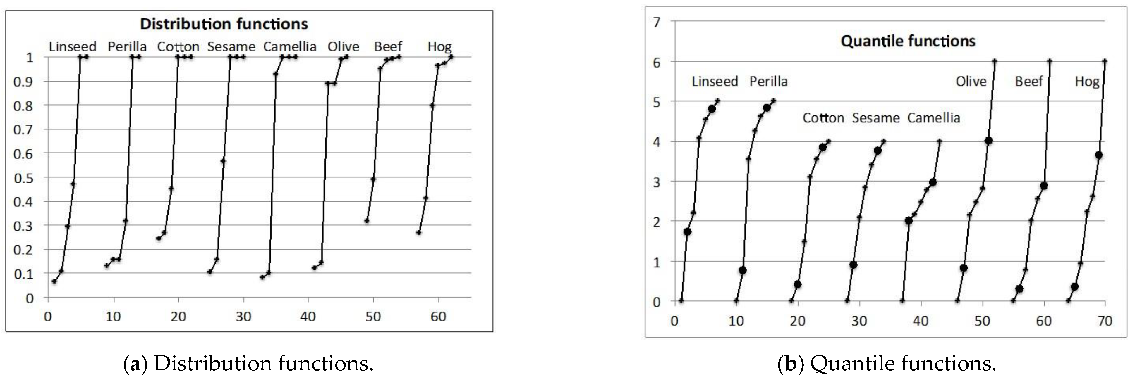
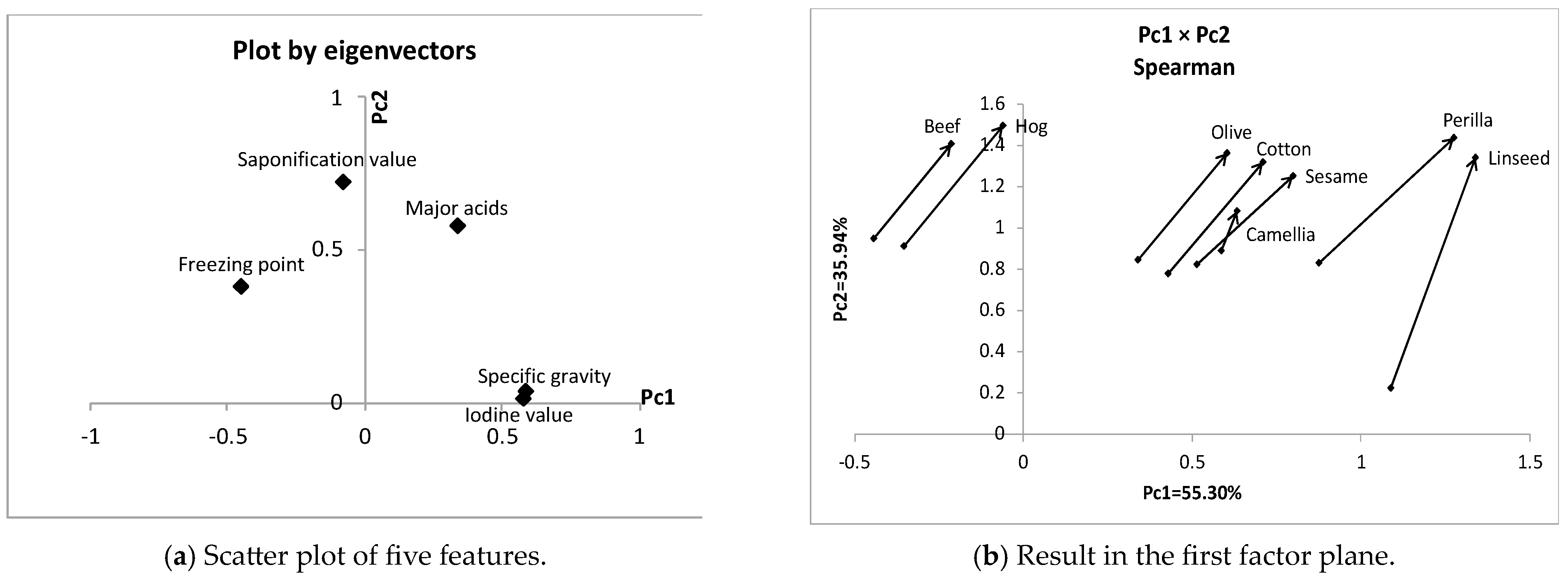
The oil data in Table 1 are composed of six plant oils and two animal fats described using four interval-valued features and one nominal multivalued feature. Here, we used the composition table in Table 2 for major acids. Each object is composed of acids from the ordered acids by molecular weight. For each object, we assumed a unit interval for each component acid assuming uniform distribution. Figure 4a shows the obtained cumulative distribution functions, and Figure 4b contains the corresponding quantile functions. The last column of Table 2 features seven quantiles calculated for each object. Table 3 shows the oil data described using five interval values. For major acids, we cut 0% and 100% quantiles to clarify the distinctions between objects, and we regarded 10% and 90% quantiles as the new 0% and 100% quantiles. Table 4 features the first two principal components for the oil data in Table 3. The two principal components have very high contribution ratios. In this example, the first principal component is not the size factor. Specific gravity and iodine value have very large positive weights.
Figure 5a shows the mutual position of five features, and specific gravity and iodine value are highly covariate. In Figure 5b, each object is represented by an arrow line connecting the minimum quantile vector and the maximum quantile vector. Beef and hog are isolated from plant oils. On the other hand, linseed and perilla have larger concept sizes and are separated from the other four plant oils.
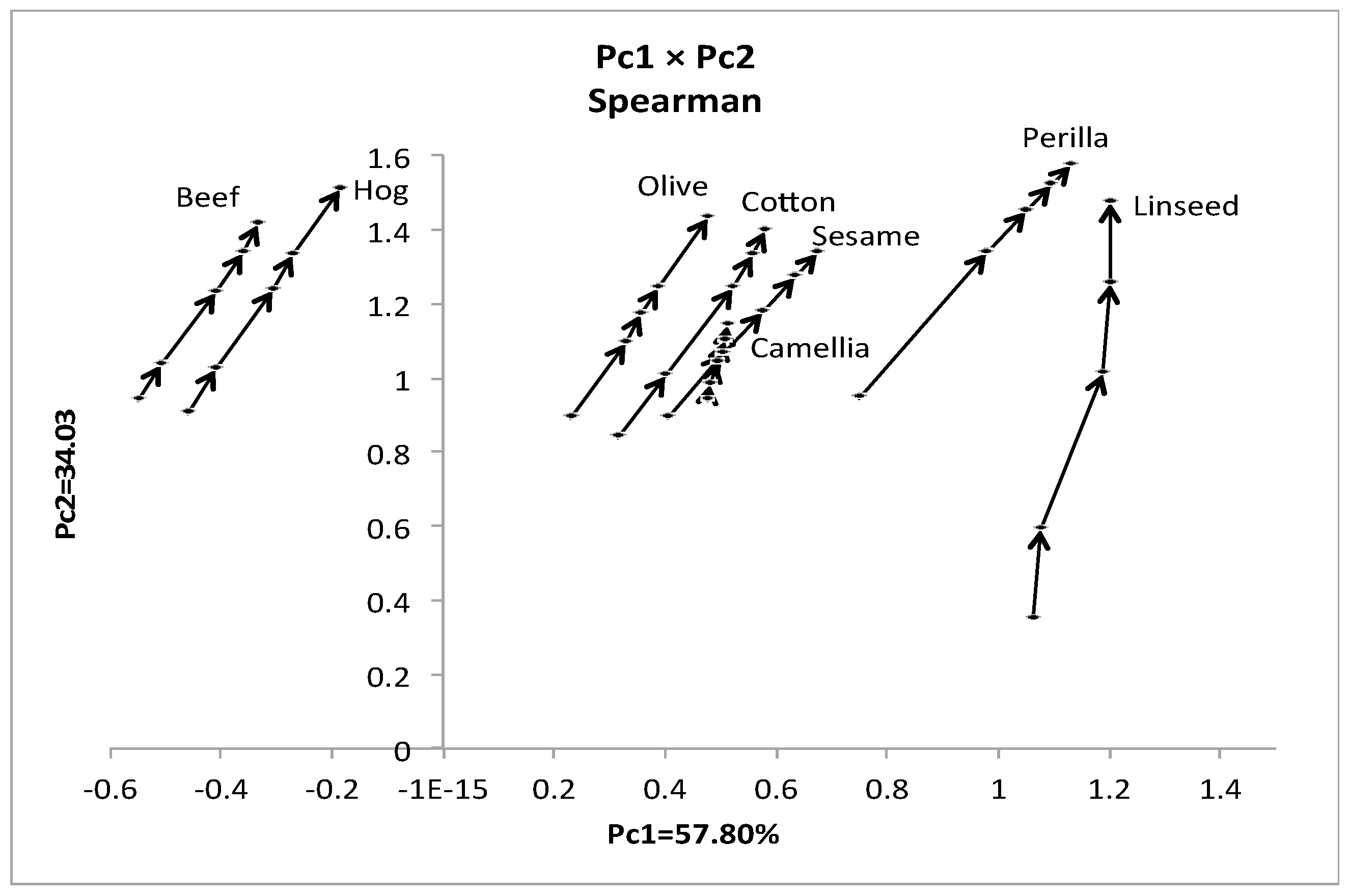
Table 5 demonstrates part of the oil data for quartile representation. We obtained quartiles for four interval feature values assuming uniform distributions. Table 6 reveals the first two principal components for the quartile case. The two principal components, again, have very high contribution ratios and are very similar to the results of Table 4. Figure 6 shows eight objects represented by four connected arrow lines from the minimum quantile vector to the maximum quantile vector. The quartile representation affects the shapes of objects, as indicated by the arrow lines.
3.1.2. Dual PCA of Oil Data
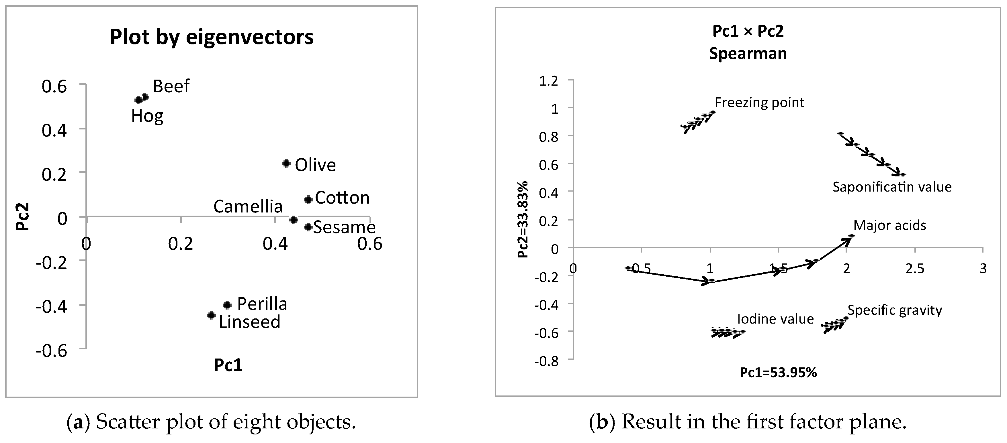
In the oil data by quartile representation, we used data in the form of (8 × 5 quantile values) × (5 variables). We replaced the positions of eight objects and five variables as (5 × 5 quantile values) × (8 objects). Using the factorization of Spearman’s 8 × 8 rank order correlation matrix, we obtained the results in Table 7. The sum of the contribution ratios is large, and the first principal component is the size factor in dual PCA. The scatter plot of Figure 7a is consistent with the results in Figure 5b and Figure 6. In Figure 7b, specific gravity and iodine value have small concept sizes and are mutually covariate. Similarly, freezing point is covariate with saponification value. In between these two groups, major acids shows the largest concept size.
3.1.3. PCA of Hardwood Data
The data were extracted from the US Geological Survey (Climate—Vegetation Atlas of North America) [23]. The number of objects is ten, and the number of features is eight. Table 8 shows quantile values for the selected ten hardwoods under the variable mean annual temperature (ANNT). For example, the existence probability of Acer East is 0% under −2.3 °C and 10% in the range −2.3~0.6 °C, etc. We selected the following eight variables to describe the objects (hardwood). The data formats for other variables F2~F8 are the same as those in Table 8.
- F1: Annual temperature (ANNT) (°C).
- F2: January temperature (JANT) (°C).
- F3: July temperature (JULT) (°C).
- F4: Annual precipitation (ANNP) (mm).
- F5: January precipitation (JANP) (mm).
- F6: July precipitation (JULP) (mm).
- F7: Growing degree days on 5 °C base × 1000 (GDC5).
- F8: Moisture index (MITM).
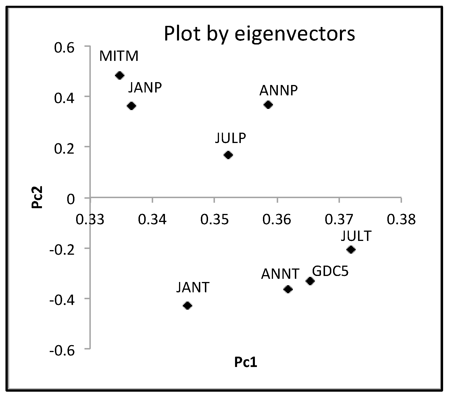
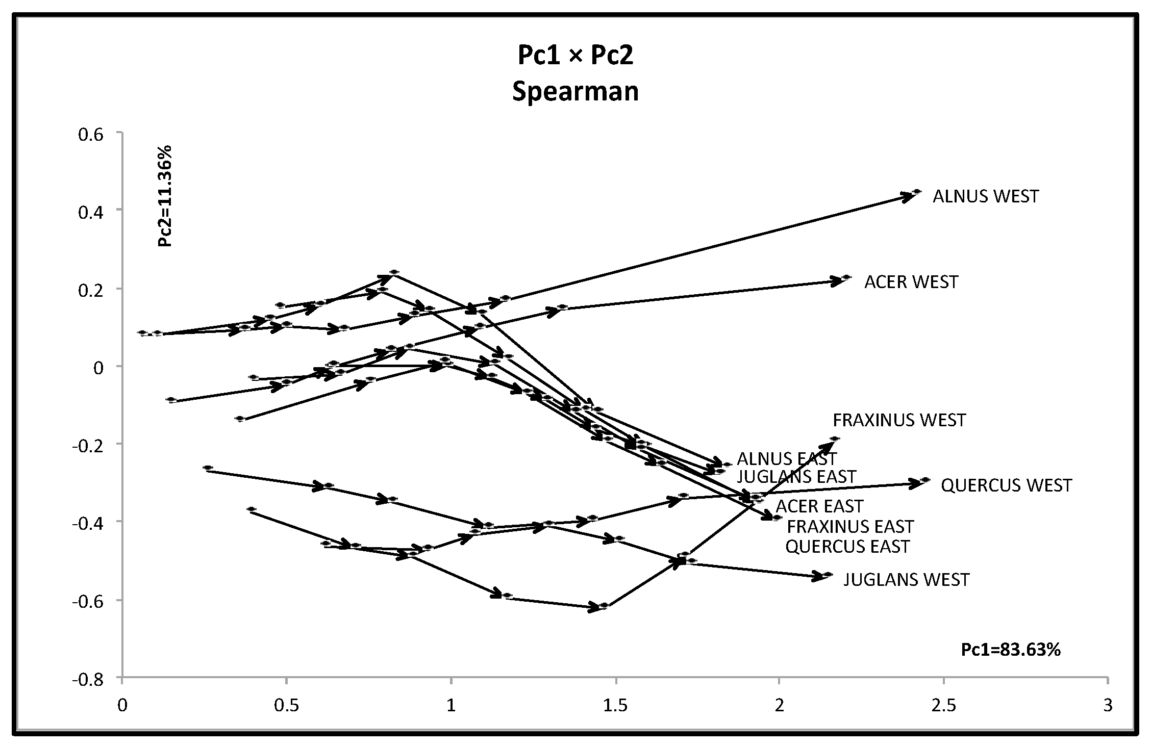
The hardwood data are numerical data of the size {(10 objects) × (7 quantile values)} × (8 variables). Using the factorization of Spearman’s 8 × 8 rank order correlation matrix, we obtained the results in Table 9. Figure 8 shows the mutual positions of eight variables by two eigen vectors. We have two groups {ANNP, JANP, JULP, and MOISTURE} and {ANNT, JANT, JULT, and GDC5}. Figure 9 shows the mutual positions of ten objects in the first factor plane. Each hardwood is represented by six arrow lines connecting the minimum quantile vector to the maximum quantile vectors.
We should note the following facts for the PCA results:
- The first principal component is the size factor and the second is the shape factor, and the sum of their contribution ratios is very high.
- East hardwoods show similar line graphs, and the maximum quantile vectors take mutually near positions.
- West hardwoods are separated into two groups: {ACER WEST and ALNUS WEST} and {FRAXINUS WEST, JUGLANS WEST, and QUERCUS WEST}. The last arrow lines are very long, especially for ACER WEST and ALNUS WEST.
3.1.4. Dual PCA of Hardwood Data
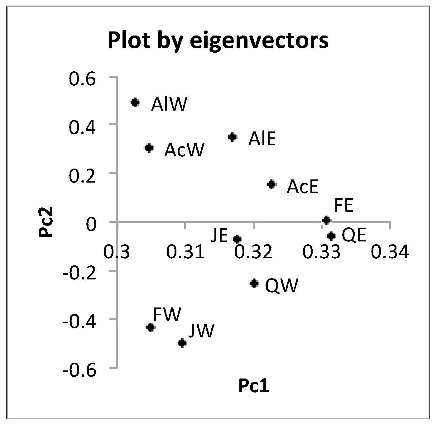
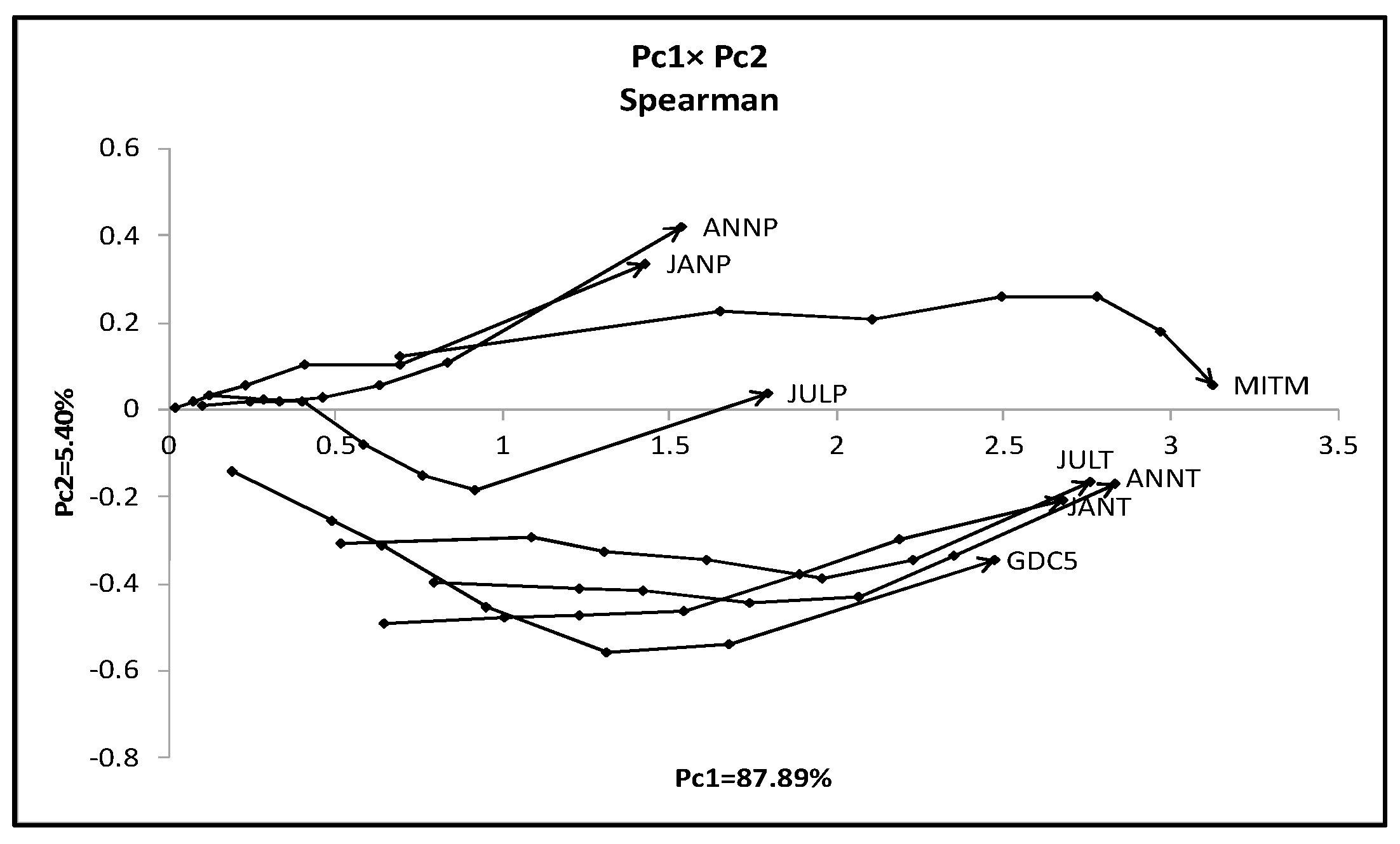
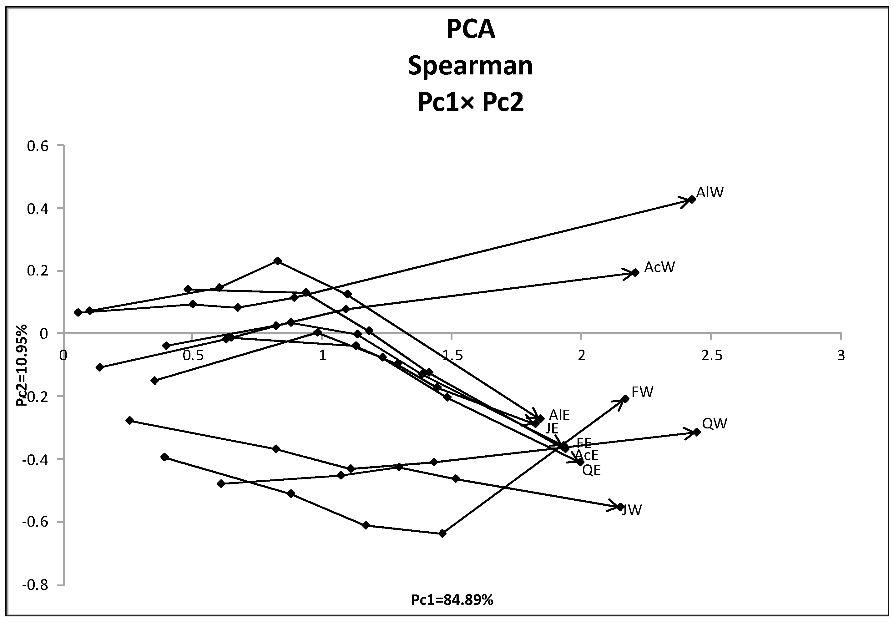
We changed the places of objects and variables in the hardwood data. Then, we applied the quantile method of PCA to the dual data in the form of {(8 variables) × (7 quantile values)} × (10 objects). Table 10 contains the first two principal components for the dual data, and Figure 10 shows the mutual positions of ten hardwoods by two eigenvectors. West hardwoods are separated, again, into two different groups. Figure 11 shows the mutual position of eight variables in the first factor plane. Each variable is represented by a series of six-line segments connecting the minimum quantile vector to the maximum quantile vector.
We should note the following facts for the result of dual PCA:
- The first principal component is the size factor and the second is the shape factor, and the sum of their contribution ratios is very high.
- We have two groups: {ANNP, JANP, JULP, and MITM} and {ANNT, JANT, JULT, and GDC5}. MITM and GDC5 have very long line graphs compared with the other members in each group.
3.2. Unsupervised Feature Selection Using Hierarchical Conceptual Clustering
This section describes our algorithm of hierarchical conceptual clustering and an exploratory method for unsupervised feature selection based on compactness.
Let U = {ω1, ω2, …, ωN} be the given set of objects, and let each object ωi be described using a set of histograms Ei = Ei1 × Ei2 × ··· × Eip in the feature space Rp. We assumed that all histogram values for all objects have the same number, m, of quantiles. We also assumed the same bin probabilities for all histogram values to keep the monotone property in Proposition 5 and Proposition 6 (3).
3.2.1. Analysis of Oil Data
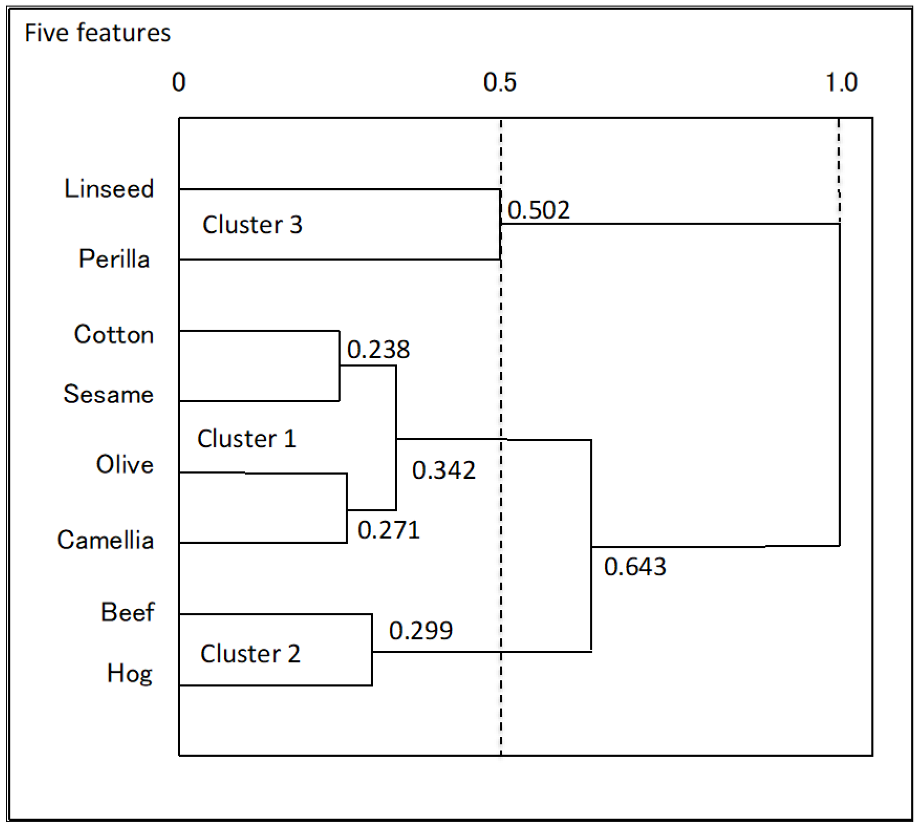
We applied the hierarchical conceptual clustering (HCC) algorithm [13] to the oil data in Table 3. In this data, each object is described using interval values, i.e., histograms having a single bin. The dendrogram in Figure 12 shows three explicit clusters (linseed, perilla), (cotton, sesame, olive, camellia), and (beef, hog).
Table 11 summarizes the values of the average compactness for each feature in each clustering step. As clarified by bold format numbers, the most robustly informative features are specific gravity and iodine value until step 6.
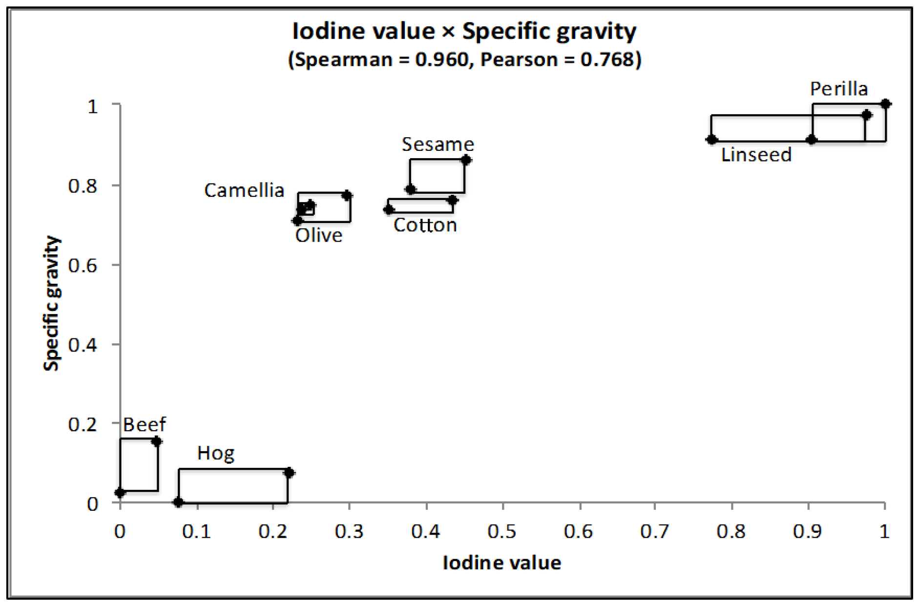
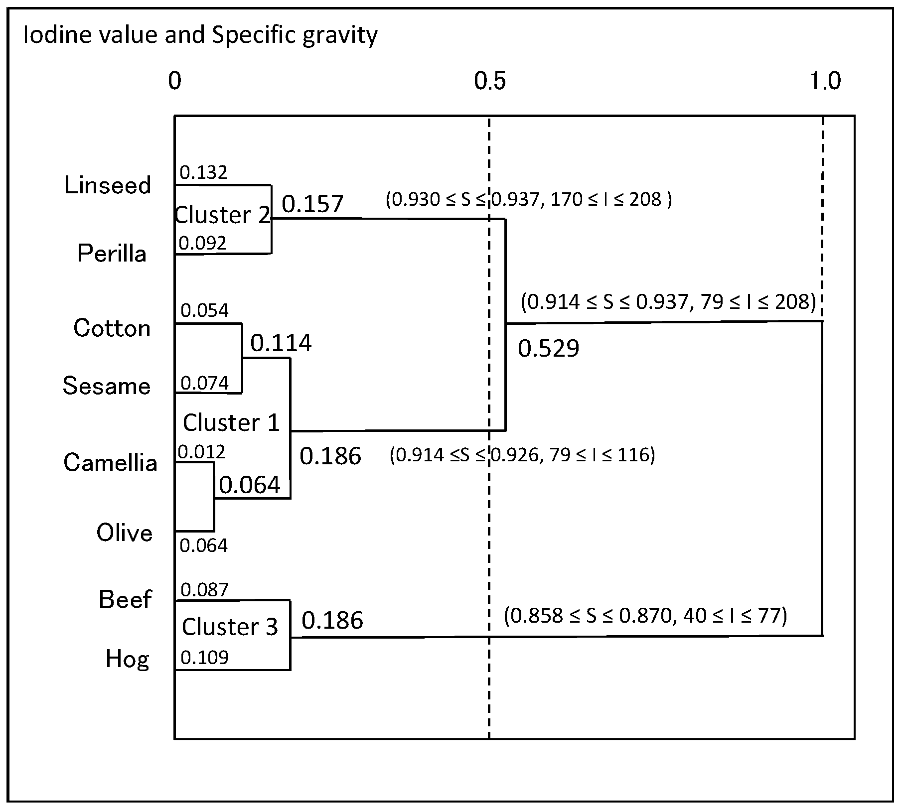
Figure 13 shows the scatter diagram of the oil data for the two selected robustly informative features. This figure, again, shows three distinct clusters (linseed, perilla) and (cotton, sesame, camellia, olive), and (beef, hog). They exist in locally limited regions, and they are organized in a geometrically thin structure with respect to the selected features. Figure 14 shows the dendrogram with concept descriptions of clusters with respect to specific gravity and iodine value. This dendrogram clarifies two major clusters, plant oils and fats, in addition to three distinct clusters, and the compactness takes smaller values compared with the dendrogram in Figure 12. We should note that compactness plays the role of the similarity measure between objects and/or clusters, the role of the cluster quality measure, and the role of the feature effectiveness criterion.
3.2.2. Analysis of Hardwood Data
To maintain the monotone property in Propositions 5 and 6 (3), we assumed quartile representation for the hardwood data. Figure 15 is the result of PCA for the quartile case. After the removal of 10% and 90% quantiles, the lengths of the first and the last line segments greatly increased compared with the result in Figure 9, especially for the west hardwoods.
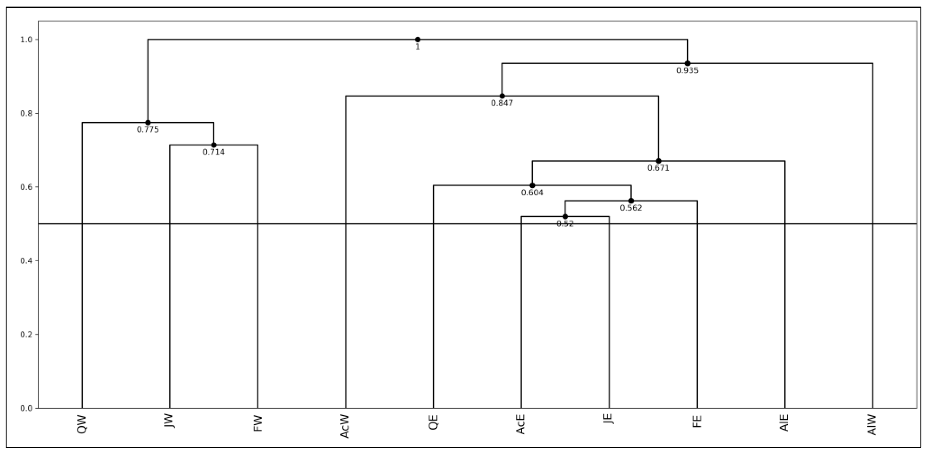
Figure 16 is the result of our HCC using compactness. In this dendrogram, HCC generated a cluster of east hardwoods in the order ((((AcE, JE), FE), QE), AlE), and ((JW, FW), QW). Then, AcW was merged into the cluster of east hardwoods with a compactness of 0.847, and AlW was merged further with a compactness of 0.935. Because the compactness of east hardwoods is 0.671, AcW and AlW are mutually similar compared with the east hardwoods. As a result, we have three clusters (AcW, AlW), (AcE, AlE, FE, JE, QE), and (FW, JW, QW). The PCA result in Figure 15 also supports these clusters.
Table 12 shows the average compactness for each feature and clustering step. The most robustly informative feature is ANNP, then JULP. However, we should note that JANT is also important in steps 7 and 8.
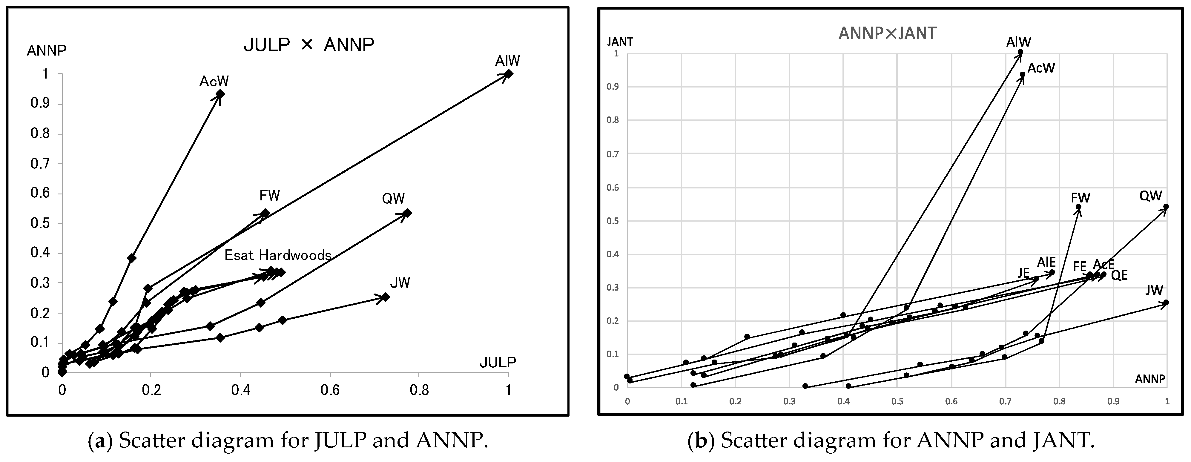
Figure 17a,b show the scatter diagrams of ten hardwoods by informative feature. Figure 17b is very similar to the PCA result in Figure 15. We should note, again, that the compactness contributed to the selection of the important features. We should also note that the minimum quantile vectors and the maximum quantile vectors describe the differences between objects and/or clusters in the scatter diagrams under the selected informative features.
3.3. Lookup Table Regression Model
This section describes the lookup table regression model (LTRM) for histogram-valued symbolic data [21,22]. For the given symbolic data table of the size (N objects) × (p variables), we represented each object using (m + 1) p-dimensional quantile vectors, where m is a preselected integer number. To the new numerical data table of the size {N × (m + 1) quantile values} × (p variables), we applied the monotone blocks segmentation (MBS) algorithm. The MBS interchange N × (m + 1) rows were organized according to the values of the selected response variable, from smallest to largest. For each of the remaining p − 1 explanatory variables, i.e., columns, MBS executed the segmentation of variable values into blocks so that the generated blocks, i.e., interval values, satisfied the monotone property. MBS discarded columns that had only a single block. Therefore, MBS detected monotone covariate relations existing between the response variable and explanatory variable(s). Finally, MBS obtained a lookup table of the size N′ × p′, where N′ < N × (m + 1) and p′ < p. Each element of the table was an interval value corresponding to the segmented block. We realized the interval value estimation rule for the response variable by searching for the nearest element in the lookup table.
3.3.1. Illustration by Oil Data
We used the oil data in Table 3 to describe the basic ideas of MBS and LTRM. In these data, each of eight objects is described using five interval values. Because an interval is a special histogram composed of one bin, we split each object into two sub-objects, the minimum sub-object and the maximum sub-object, described using five-dimensional quantile vectors, i.e., the minimum quantile vector and the maximum quantile vector. Table 13 contains the obtained quantile representation of our numerical data of the size (8 × 2 quantile values) × (5 variables).
In this example, we selected iodine value as the response variable and the remaining four as explanatory variables. In Table 14, we interchanged the given sixteen quantile vectors, according to iodine value, from a minimum value of 40 to a maximum value of 208. Then, we segmented each column into blocks to satisfy the monotone property. Because the saponification value is composed of a single block, we omitted this from the explanatory variables. Specific gravity is the most strongly connected to the response variable. In the previous section, we obtained the data in Figure 14 using the unsupervised feature selection method. MBS also has a feature selection capability under monotone covariate relations between the response and explanation variables.
Table 15 contains the obtained lookup table, in which several intervals are composed of reduced interval values. Based on this lookup table, we can estimate the iodine value for each object by using specific gravity and freezing point.
The estimation rule used here is as follows:
Let [a1, a2] be the value of an explanatory variable of the given object.
- If [a1, a2] is included in an interval, [b1, b2], of the explanatory variable in the lookup table, we select the corresponding value, [c1, c2], of the response variable as the estimated value.
- If the minimum value, a1, is included in an interval, [b1, b2], corresponding to the response value, [c1, c2], and the maximum value, a2, is included in a different interval, [b3, b4], corresponding to the response value [c3, c4]. Then we determine that the minimum response value of c1 or c2 according to a1 is near b1 or b2. Similarly, we determine that the maximum response value of c3 or c4 according to a2 is near b3 or b4.
For example, the specific gravity of cotton is [0.916, 0.918] and is included in [0.916, 0.920]. Hence, the estimated iodine value is [80, 113]. On the other hand, the specific gravity of sesame is [0.920, 0.926]. The minimum value of 0.920 suggests the maximum value 113 of the response variable value [80, 113]. On the other hand, the maximum value of 0.926 suggests the value 116 of the response value [116, 116]. As a result, the estimated iodine value is [113, 116]. Table 16 summarizes our estimated result.
3.3.2. Illustration by Hardwood Data
In Section 3.1.3, we applied PCA to the hardwood data of the size (10 × 7 quantile values) × (8 variables), and we recognized three clusters, (AcW, AlW), (AcE, AlE, FE, JE, QE), and (FW, JW, QW), on the first factor plane. On the other hand, using dual PCA, we found two groups of features, {ANNP, JANP, JULP, MITM} and {ANNT, JANT, JULT, GDC5}, in which MITM and GDC5 show very long line graphs in each group.
In this example, we selected GDC5 as the response variable and the remaining seven as explanatory variables. Then, we applied MBS to the data of the size (10 × 7 quantile values) × (8 variables). MBS selected only ANNT, JANT, and JULT as explanatory variables, and we obtained a lookup table, which can be seen in Table 17.
In this table, ANNT shows the strongest connection to the response variable GDC5. We used the test data in Table 18 to check the estimation ability of our lookup table. Table 19 summarizes the estimated result for our test data. In the range [0.1, 2.5] of GDC5, the result requires further improvement because the PCA result in Figure 15 suggests the use of clustering.
Under the assumption of quartiles, we applied HCC to the hardwood data, and we obtained the dendrogram in Figure 16. From the results in Figure 15 and Figure 16, we supposed three clusters, C1 = (AcW, AlW), C2 = (AcE, AlE, FE, JE, QE), and C3 = (FW, JW, QW), in the following discussion.
We applied MBS to each of three clusters, C1, C2 and C3. Table 20, Table 21 and Table 22 feature lookup tables for these three clusters. In Table 20, JULT contributes to the range [0.1, 1.1] of GDC5. On the other hand, in Table 21 and Table 22, ANNT is strongly connected to the whole range of GDC5.
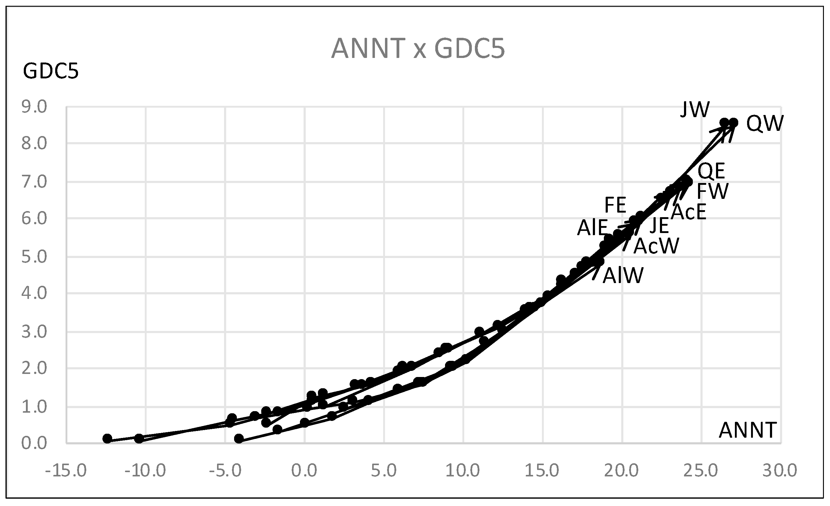
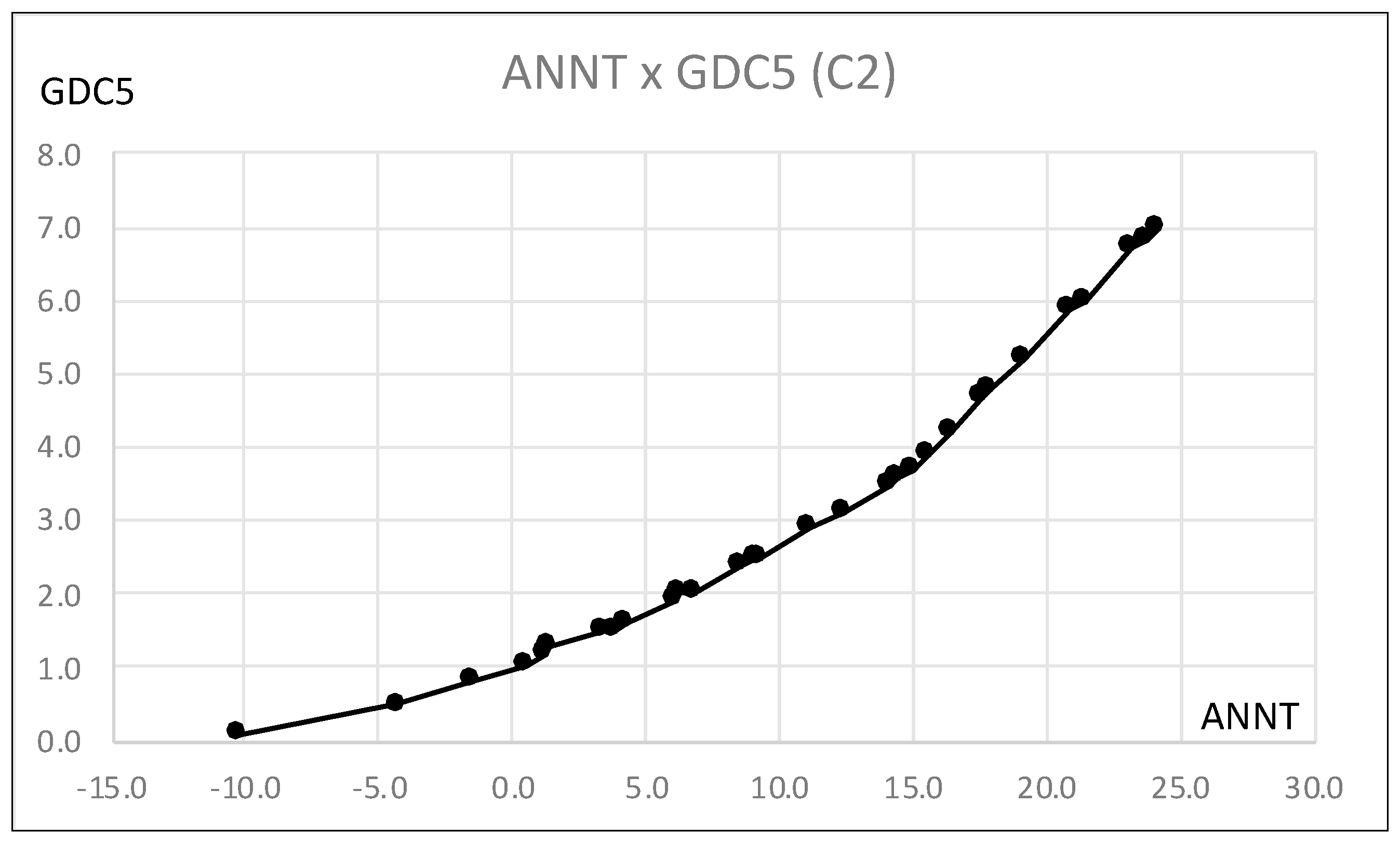
Figure 18 shows the scatter diagram of the hardwood data for ANNT and GDC5, in which all hardwoods exist in a narrow region. We used the estimation of GDC5 by ANNT for cluster C2 because the lookup table for C2 covers the widest range of ANNT compared with the other lookup tables. Figure 19 shows the graph of GDC5 for ANNT under cluster C2, and Table 23 presents the estimation result for the test data. We could have a better estimation result compared to the result in Table 19.
4. Conclusive Summary
The quantile method is a unified quantification method for histogram-valued symbolic data. We retraced and summarized three research categories: principal component analysis using the monotone property of quantile values, hierarchical conceptual clustering and unsupervised feature selection using the compactness measure, and look up table regression model using monotone blocks segmentation (MBS). In the following sections, we summarize our results.
4.1. PCA and Dual PCA
For each object, (m + 1) quantile values of each variable satisfied the monotone property. Based on this property, PCA was realized using the eigenvalue problem of the Spearman correlation matrix.
4.1.1. Analysis of Oil Data
In the PCA of the oil data, three explicit clusters (beef, hog), (olive, camellia, cotton, sesame), and (linseed, perilla) were obtained in the factor plane using the first two principal components with a high contribution ratio. Linseed and perilla have larger line graphs compared with the other objects. The quartile representation affected the shapes of the objects, especially linseed. In the dual PCA using quartile representation, three groups, (freezing point, saponification value), (major acids), and (specific gravity, iodine value) were placed in different positions on the factor plane using the first two principal components with a high contribution ratio. The specific gravity and iodine values have very small concept sizes and are in mutually near positions. Major acids has a very large line graph and is located between the two other groups.
4.1.2. Analysis of Hardwood Data
In the PCA of hardwood data, three clusters, (AcW, AlW), (AcE, AlE, FE, JE, QE), and (FW, JW, QW), were obtained on the factor plane using the first two principal components with a high contribution ratio. East hardwoods have similar shapes in a narrow region. On the other hand, west hardwoods, especially the maximum quantile vectors, were spread in a wide range on the factor plane. In the dual PCA, two groups (ANNP, JANP, JULP, MITM) and (ANNT, JANT, JULT, GDC5) were obtained on the factor plane using the first two principal components with a high contribution ratio. MITM and GDC5 have very large line graphs in their respective groups.
4.2. Hierarchical Conceptual Clustering (HCC) and Unsupervised Feature Selection
The HCC algorithm is based on compactness under the assumption of equal bin probabilities. Compactness is the concept size of the merged concept of two objects and/or clusters. Compactness takes a 0–1 normalized value and satisfies the monotone property, i.e., the merged concept size is larger than the concept sizes of the two given objects and/or clusters. In each step of our hierarchical conceptual clustering, two objects and/or clusters were merged to minimize compactness. This required the two merged objects and/or clusters to be mutually similar and have small concept sizes. In this sense, compactness plays the role of similarity measure between objects and/or clusters. On the other hand, to minimize the merged concept size is equivalent to maximizing the dissimilarity of the merged concept from the whole concept. Therefore, compactness plays the role of cluster quality. In each clustering step, we evaluated the average compactness of objects and/or clusters for each variable. Then, the informative features took smaller values through the successive clustering steps. Therefore, compactness also plays the role of feature effectiveness criterion. This fact greatly simplified the task of unsupervised feature selection.
4.2.1. Analysis of Oil Data
In the dendrogram of the oil data using the HCC algorithm, three explicit clusters, (beef, hog), (olive, camellia, cotton, sesame), and (linseed, perilla) are recognized again as PCA results. However, (linseed, perilla) is isolated from other plant oils in the obtained dendrogram. From the results of average compactness evaluated for each variable and each clustering step, the most robustly informative variables are specific gravity and iodine value. The dual PCA and scatter diagram of eight oils on the plane using these informative variables also support the obtained result. In the dendrogram of the oil data using two informative features, three clusters have smaller concept sizes than those in the dendrogram using five variables, and they have mutually similar concept sizes. Furthermore, the cluster (linseed, perilla) is merged with the cluster of other plant oils.
4.2.2. Analysis of Hardwood Data
The dendrogram of the hardwood data using the HCC algorithm shows two large clusters, (FW, JW, QW) and (AcE, AlE, FE, JE, QE, AcW, AlW), at step 8. The results of average compactness for each variable and each clustering step show the facts: ANNP is informative during steps 1~8, then, JULP is important during steps 3~7, and JANT is important in steps 7~8. Five east hardwoods exist in a narrow region on the plane using ANNP and JULP, and west hardwoods spread out widely on the same plane. On the other hand, on the plane using ANNP and JANT, we have three clusters, (AcW, AlW), (AcE, AlE, FE, JE, QE), and (FW, JW, QW), and the scatter diagram is very similar to the result of PCA on the factor plane using the first two principal components.
4.3. Lookup Table Regression Model (LTRM)
In the LTRM, we used the monotone blocks segmentation (MBS) algorithm. When each of N objects was represented by (m + 1) p-dimensional quantile vectors, MBS interchanged N × (m + 1) rows of the data table according to the values of the selected response variable, from smallest to largest. For each of the remaining p − 1 explanatory variables, i.e., columns, MBS executed the segmentation of variable values into blocks so that the generated blocks, i.e., interval values, satisfied the monotone property. The MBS discarded single-block columns and obtained a lookup table of the size N′ × p′, where N′ < N × (m + 1) and p′ < p. We realized the interval estimation rule for the response variable by searching for the nearest element in the lookup table.
4.3.1. Lookup Table of Oil Data
When each object was represented by the minimum and maximum quantile vectors, we applied MBS to the data under the assumption that iodine value was the response variable and the remaining four were explanatory variables. As a result, we obtained a lookup table composed of three explanatory variables: specific gravity, freezing point, and major acids. Specific gravity is the most important variable for explaining iodine value, and this result is supported by the unsupervised feature selection for the oil data.
4.3.2. Lookup Table of the Hardwood Data
We applied MBS to the hardwood data described using seven quantile values under the assumption that GDC5 was the response variable and the remaining seven were explanatory variables. We obtained the lookup table, which is composed of three explanatory variables: ANNT, JANT, and JULT. Among these, ANNT had the strongest connection to the response variable. This result is supported by the dual PCA for the hardwood data. We applied the test data, which is composed of six hardwoods, to the obtained lookup table. In the range [0.1, 2.5] of GDC5, the result required further improvement. The result of the PCA for the hardwood data also suggested the use of clustering. We applied MBS to each of three clusters, i.e., two west hardwood clusters and one east hardwood cluster. The three obtained lookup tables and the scatter diagram of hardwoods using GDC5 and ANNT suggested the use of the lookup table for the east hardwood cluster because this lookup table covers the widest range of GDC5. In fact, we could have the improved estimation results for our test data using the lookup table using the east hardwood cluster.
As a concluding remark, we should note that three research categories using the quantile method are mutually cooperative for analyzing the given distributional data under the common monotone property of quantiles.
Funding
This work was supported by JSPS KAKENHI (Grants-in-Aid for Scientific Research) Grant Number 25330268.
Institutional Review Board Statement
Not applicable.
Informed Consent Statement
Not applicable.
Data Availability Statement
No new data were created or analyzed in this study. Data sharing is not applicable to this article.
Acknowledgments
The author thanks to Edwin Diday for his valuable comments on the quantile method.
Conflicts of Interest
The author declares no conflicts of interest.
References
- Bock, H.-H.; Diday, E. Analysis of Symbolic Data; Springer: Berlin/Heidelberg, Germany, 2000. [Google Scholar]
- Billard, L.; Diday, E. Symbolic Data Analysis: Conceptual Statistics and Data Mining; Wiley: Chichester, UK, 2007. [Google Scholar]
- Billard, L.; Diday, E. Regression analysis for interval-valued data. In Data Analysis, Classification and Related Methods, Proceedings of the Conference of the International Federation of Classification Societies (IFCS’00); Springer: Berlin/Heidelberg, Germany, 2000; pp. 347–369. [Google Scholar]
- Diday, E. Thinking by classes in data science: The symbolic data analysis paradigm. WIREs Comput. Stat. 2016, 8, 172–205. [Google Scholar] [CrossRef]
- Lauro, N.C.; Verde, R.; Irpino, A. Principal component analysis of symbolic data described by intervals. In Symbolic Data Analysis and SODAS Software; Diday, E., Noirhomme-Fraiture, M., Eds.; Wiley: Chichester, UK, 2008; pp. 279–311. [Google Scholar]
- Ichino, M. General metrics for mixed features—The Cartesian space theory for pattern recognition. In Proceedings of the International Conference on Systems, Man, and Cybernetics, Beijing, China, 8–12 August 1988. [Google Scholar]
- Ichino, M.; Yaguchi, H. Generalized Minkowski metrics for mixed feature-type data analysis. IEEE Trans. Syst. Man Cybern. 1994, 24, 698–708. [Google Scholar] [CrossRef]
- Ichino, M. Symbolic PCA for histogram-valued data. In Proceedings of the IASC 2008, Yokohama, Japan, 5–8 December 2008. [Google Scholar]
- Ichino, M. The quantile method of symbolic principal component analysis. Stat. Anal. Data Min. 2011, 4, 184–198. [Google Scholar] [CrossRef]
- Irpino, A.; Verde, R. A new Wasserstein based distance for the hierarchical clustering of histogram symbolic data. In Data Science and Classification; Springer: Berlin/Heidelberg, Germany, 2006; pp. 185–192. [Google Scholar]
- de Carvalho, F.D.A.T.; De Souza, M.C.R. Unsupervised pattern recognition models for mixed feature-type data. Pattern Recognit. Lett. 2010, 31, 430–443. [Google Scholar] [CrossRef]
- Umbleja, K.; Ichino, M.; Yaguchi, H. Hierarchical conceptual clustering based on the quantile method for identifying microscopic details in distributional data. Adv. Data Anal. Classif. 2021, 15, 407–436. [Google Scholar] [CrossRef]
- Ichino, M.; Umbleja, K.; Yaguchi, H. Unsupervised feature selection for histogram-valued symbolic data using hierarchical conceptual clustering. Stats 2021, 4, 359–384. [Google Scholar] [CrossRef]
- Verde, R.; Irpino, A. Ordinary least squares for histogram data based on Wasserstein distance. In Proceedings of the COM-STAT, Paris, France, 22–27 August 2010; Lechevallier, Y., Saporta, G., Eds.; Physica-Verlag: Heidelberg, Germany, 2010; pp. 581–589. [Google Scholar]
- Irpino, A.; Verde, R. Linear regression for numeric symbolic variables: Ordinary least squares approach based on Wasserstein Distance. Adv. Data Anal. Classif. 2015, 9, 81–106. [Google Scholar] [CrossRef]
- Neto, E.D.; De Carvalho, F.D. Center and range method for fitting a linear regression model for symbolic interval data. Comput. Stat. Data Anal. 2008, 52, 1500–1515. [Google Scholar] [CrossRef]
- Neto, L.; Carvalho, D. Constrained linear regression models for symbolic interval-valued variables. Comput. Stat. Data. Anal. 2010, 54, 333–347. [Google Scholar] [CrossRef]
- Neto, L.; Cordeiro, M.; Carvalho, D. Bivariate symbolic regression models for interval-valued variables. J. Stat. Comput. Simul. 2011, 81, 1727–1744. [Google Scholar] [CrossRef]
- Dias, S.; Brito, P. Linear regression model with Histogram-valued variables. Stat. Anal. Data Min. 2015, 8, 75–113. [Google Scholar] [CrossRef]
- Dias, L.; Brito, P. (Eds.) Analysis of Distributional Data; CRC Press: Boca Raton, FL, USA, 2022. [Google Scholar]
- Ichino, M. The lookup table regression model for symbolic data. In Proceedings of the Data Sciences Workshop, Paris-Dauphin University, Paris, France, 12–13 November 2015. [Google Scholar]
- Ichino, M. The lookup table regression model for histogram-valued symbolic data. Stats 2022, 5, 1271–1293. [Google Scholar] [CrossRef]
- Histogram Data by the U.S. Geological Survey, Climate-Vegetation Atlas of North America. Available online: http://pubs.usgs.gov/pp/p1650-b/ (accessed on 11 November 2010).
Figure 1.
Cumulative distribution function and cut point probabilities.

Figure 2.
Representation of objects and bin rectangles in the quartile case.

Figure 3.
A property of compactness.

Figure 4.
Cumulative distribution functions and their corresponding quantile functions.

Figure 5.
Result of PCA for the interval-valued oil data.

Figure 6.
Result of PCA for quartile case.

Figure 7.
Result of dual PCA for the oil data.

Figure 8.
Scatter plot of eight features by two eigenvectors.

Figure 9.
Result of PCA for the hardwood data.

Figure 10.
Scatter plot of ten hardwoods by two eigenvectors.

Figure 11.
Result of dual PCA for the hardwood data.

Figure 12.
Result of HCC for oil data (five features).

Figure 13.
Scatter diagram using two informative features.

Figure 14.
Result of HCC for oil data using iodine value and specific gravity.

Figure 15.
Result of PCA for hardwood data (quartile case).

Figure 16.
Result of HCC for hardwood data (eight features).

Figure 17.
Scatter diagrams for the selected informative features.

Figure 18.
Scatter diagram of hardwood data for ANNT and GDC5.

Figure 19.
Estimation of GDC5 by ANNT for cluster C2.


| Object | Specific Gravity | Freezing Point | Iodine Value | Saponification Value | Major Acids |
|---|---|---|---|---|---|
| Linseed | [0.930, 0.935] | [−27, −18] | [170, 204] | [118, 196] | L, Ln, O, P |
| Perilla | [0.930, 0.937] | [−5, −4] | [192, 208] | [188, 197] | L, Ln, P, S |
| Cotton | [0.916, 0.918] | [−6, −1] | [99, 113] | [189, 198] | L, O, P, S |
| Sesame | [0.920, 0.926] | [−6, −4] | [104, 116] | [187, 193] | L, O, P, S |
| Camellia | [0.914, 0.917] | [−21, −15] | [80, 82] | [189, 193] | L, O, P, S |
| Olive | [0.914, 0.919] | [0, 6] | [79, 90] | [187, 196] | Ln, O, P, S, A |
| Beef | [0.860, 0.870] | [30, 38] | [40, 48] | [190, 199] | L, Ln, O, P, S, A |
| Hog | [0.858, 0.864] | [22, 32] | [53, 77] | [190, 202] | L, Ln, O, P, S, A |
L: linoleic acid, Ln: linolenic acid, O; oleic acid, P: palmitic acid, S: stearic acid, A: archaic acid.
Table 2.
Composition table of major acids.
| Object | Palmitic Acid C16:0 | Stearic Acid C18:0 | Oleic Acid C18:1 | Linoleic Acid C18:2 | Linolenic Acid C18:3 | Arachic Acid C20:0 | [0, 10%, 25%, 50%, 75%, 90%, 100%] |
|---|---|---|---|---|---|---|---|
| Linseed | 0.07 | 0.04 | 0.19 | 0.17 | 0.53 | 0.00 | [0, 1.75, 2.21, 4.06, 4.53, 4.81, 5] |
| Perilla | 0.13 | 0.03 | 0.00 | 0.16 | 0.68 | 0.00 | [0, 0.77, 3.56, 4.26, 4.63, 4.85, 5] |
| Cotton | 0.24 | 0.02 | 0.18 | 0.55 | 0.00 | 0.00 | [0, 0.42, 1.50, 3.11, 3.56, 3.84, 4] |
| Sesame | 0.11 | 0.05 | 0.41 | 0.43 | 0.00 | 0.00 | [0, 0.91, 2.09, 2.83, 3.42, 3.77, 4] |
| Camellia | 0.08 | 0.02 | 0.82 | 0.07 | 0.00 | 0.00 | [0, 2.00, 2.18, 2.49, 2.79, 2.98, 4] |
| Olive | 0.12 | 0.02 | 0.74 | 0.00 | 0.10 | 0.01 | [0, 0.83, 2.15, 2.49, 2.82, 4.02, 6] |
| Beef | 0.32 | 0.17 | 0.46 | 0.03 | 0.01 | 0.01 | [0, 0.31, 0.78, 2.02, 2.57, 2.89, 6] |
| Hog | 0.27 | 0.14 | 0.38 | 0.17 | 0.01 | 0.03 | [0, 0.37, 0.93, 2.24, 2.63, 3.65, 6] |
Table 3.
Oil data described using five interval values.
| Object | Specific Gravity | Freezing Point | Iodine Value | Saponification Value | Major Acids |
|---|---|---|---|---|---|
| Linseed | [0.930, 0.935] | [−27, −18] | [170, 204] | [118, 196] | [1.75, 4.81] |
| Perilla | [0.930, 0.937] | [−5, −4] | [192, 208] | [188, 197] | [0.77, 4.85] |
| Cotton | [0.916, 0.918] | [−6, −1] | [99, 113] | [189, 198] | [0.42, 3.84] |
| Sesame | [0.920, 0.926] | [−6, −4] | [104, 116] | [187, 193] | [0.91, 3.77] |
| Camellia | [0.914, 0.917] | [−21, −15] | [80, 82] | [189, 193] | [2.00, 2.98] |
| Olive | [0.914, 0.919] | [0, 6] | [79, 90] | [187, 196] | [0.83, 4.02] |
| Beef | [0.860, 0.870] | [30, 38] | [40, 48] | [190, 199] | [0.31, 2.89] |
| Hog | [0.858, 0.864] | [22, 32] | [53, 77] | [190, 202] | [0.37, 3.65] |
Table 4.
The first two principal components for the oil data in Table 3.
Table 4.
The first two principal components for the oil data in Table 3.
| Spearman | Pc1 | Pc2 |
| Eigen values | 2.77 | 1.80 |
| Contribution(%) | 55.30 | 35.94 |
| Eigen vectors | Pc1 | Pc2 |
| Specific gravity | 0.584 | 0.034 |
| Freezing point | −0.448 | 0.379 |
| Iodine value | 0.578 | 0.012 |
| Saponification value | −0.077 | 0.721 |
| Major acids | 0.343 | 0.579 |
Table 5.
Part of the oil data by quartile representation.
| Object | Specific Gravity | Freezing Point | Iodine Value | Saponification Value | Major Acids |
|---|---|---|---|---|---|
| Linseed 0 | 0.930 | −27.00 | 170.0 | 118.0 | 1.75 |
| 1 | 0.931 | −24.75 | 178.5 | 137.5 | 2.21 |
| 2 | 0.933 | −22.50 | 187.0 | 157.0 | 4.06 |
| 3 | 0.934 | −20.25 | 195.5 | 176.5 | 4.53 |
| 4 | 0.935 | −18.00 | 204.0 | 196.0 | 4.81 |
Table 6.
The first two principal components for the quartile case of the oil data.
| Spearman | Pc1 | Pc2 |
| Eigen values | 2.89 | 1.70 |
| Contribution (%) | 57.80 | 34.03 |
| Eigen vectors | Pc1 | Pc2 |
| Specific gravity | 0.570 | 0.099 |
| Freezing point | −0.457 | 0.383 |
| Iodine value | 0.562 | 0.093 |
| Saponification value | −0.190 | 0.700 |
| Major acids | 0.339 | 0.588 |
Table 7.
The first two principal components for dual PCA of the oil data.
| Spearman | Pc1 | Pc2 |
| Eigen values | 4.32 | 2.71 |
| Contribution (%) | 53.95 | 33.83 |
| Eigen vectors | Pc1 | Pc2 |
| Linseed | 0.26 | −0.45 |
| Perilla | 0.30 | −0.40 |
| Cotton | 0.47 | 0.08 |
| Sesame | 0.47 | −0.04 |
| Camellia | 0.44 | −0.02 |
| Olive | 0.42 | 0.24 |
| Beef | 0.12 | 0.54 |
| Hog | 0.11 | 0.53 |
Table 8.
The original quantile values for ANNT.
| TAXON NAME | Mean Annual Temperature (°C) | ||||||
|---|---|---|---|---|---|---|---|
| 0% | 10% | 25% | 50% | 75% | 90% | 100% | |
| ACER EAST | −2.3 | 0.6 | 3.8 | 9.2 | 14.4 | 17.9 | 24 |
| ACER WEST | −3.9 | 0.2 | 1.9 | 4.2 | 7.5 | 10.3 | 21 |
| ALNUS EAST | −10 | −4.4 | −2.3 | 0.6 | 6.1 | 15.0 | 21 |
| ALNUS WEST | −12 | −4.6 | −3.0 | 0.3 | 3.2 | 7.6 | 19 |
| FRAXINUS EAST | −2.3 | 1.4 | 4.3 | 8.6 | 14.1 | 17.9 | 23 |
| FRAXINUS WEST | 2.6 | 9.4 | 11.5 | 17.2 | 21.2 | 22.7 | 24 |
| JAGLANS EAST | 1.3 | 6.9 | 9.1 | 12.4 | 15.5 | 17.6 | 21 |
| JAGLANS WEST | 7.3 | 12.6 | 14.1 | 16.3 | 19.4 | 22.7 | 27 |
| QUERCUS EAST | −1.5 | 3.4 | 6.3 | 11.2 | 16.4 | 19.1 | 24 |
| QUERCUS WEST | −1.5 | 6.0 | 9.5 | 14.6 | 17.9 | 19.9 | 27 |
Table 9.
The first two principal components of the hardwood data.
| Spearman | Pc1 | Pc2 |
| Eigen values | 6.6908 | 0.9086 |
| Contribution (%) | 83.6346 | 11.3573 |
| Eigen vectors | Pc1 | Pc2 |
| ANNT | 0.3618 | −0.3630 |
| JANT | 0.3456 | −0.4270 |
| JULT | 0.3718 | −0.2076 |
| ANNP | 0.3585 | 0.3695 |
| JANP | 0.3366 | 0.3648 |
| JULP | 0.3522 | 0.1697 |
| GDC5 | 0.3653 | −0.3312 |
| MITM | 0.3347 | 0.4845 |
Table 10.
The first two principal components of the dual hardwood data.
| Spearman | Pc1 | Pc2 |
| Eigen values | 8.79 | 0.54 |
| Contribution (%) | 87.89 | 5.40 |
| Eigen vectors | Pc1 | Pc2 |
| AcE | 0.323 | 0.156 |
| AcW | 0.305 | 0.308 |
| AlE | 0.317 | 0.354 |
| AlW | 0.303 | 0.496 |
| FE | 0.331 | 0.008 |
| FW | 0.305 | −0.436 |
| JE | 0.318 | −0.071 |
| JW | 0.309 | −0.497 |
| QE | 0.331 | −0.056 |
| QW | 0.320 | −0.253 |
Table 11.
Average compactness of each feature in each clustering step.
| Feature | Average Compactness for Each Clustering Step | |||||||
|---|---|---|---|---|---|---|---|---|
| 0 | 1 | 2 | 3 | 4 | 5 | 6 | 7 | |
| Specific gravity | 0.066 | 0.080 | 0.091 | 0.099 | 0.114 | 0.131 | 0.475 | 1.000 |
| Freezing point | 0.090 | 0.099 | 0.154 | 0.178 | 0.204 | 0.338 | 0.631 | 1.000 |
| Iodine value | 0.090 | 0.095 | 0.109 | 0.137 | 0.185 | 0.222 | 0.339 | 1.000 |
| Saponification value | 0.202 | 0.224 | 0.254 | 0.283 | 0.327 | 0.405 | 0.560 | 1.000 |
| Major acids | 0.646 | 0.648 | 0.720 | 0.753 | 0.775 | 0.809 | 0.856 | 1.000 |
Table 12.
Average compactness of each feature in each clustering step.
| Step | Average Compactness of Each Feature | |||||||
|---|---|---|---|---|---|---|---|---|
| ANNT | JANT | JULT | ANNP | JANP | JULP | GDC5 | MITM | |
| 0 | 0.161 | 0.160 | 0.178 | 0.115 | 0.113 | 0.133 | 0.180 | 0.196 |
| 1 | 0.220 | 0.228 | 0.239 | 0.144 | 0.140 | 0.172 | 0.246 | 0.242 |
| 2 | 0.229 | 0.234 | 0.268 | 0.186 | 0.197 | 0.191 | 0.256 | 0.323 |
| 3 | 0.238 | 0.243 | 0.282 | 0.202 | 0.217 | 0.203 | 0.268 | 0.338 |
| 4 | 0.279 | 0.269 | 0.322 | 0.223 | 0.243 | 0.220 | 0.292 | 0.358 |
| 5 | 0.404 | 0.395 | 0.475 | 0.337 | 0.372 | 0.350 | 0.455 | 0.541 |
| 6 | 0.490 | 0.472 | 0.570 | 0.388 | 0.428 | 0.401 | 0.525 | 0.614 |
| 7 | 0.601 | 0.578 | 0.692 | 0.571 | 0.595 | 0.505 | 0.646 | 0.739 |
| 8 | 0.829 | 0.777 | 0.938 | 0.768 | 0.810 | 0.887 | 0.899 | 1.000 |
Table 13.
Quantile representation of oil data.
| Sub-Object | Specific Gravity | Freezing Point | Iodine Value | Saponification Value | Major Acids |
|---|---|---|---|---|---|
| Linseed 1 | 0.930 | −27 | 170 | 118 | 1.75 |
| Linseed 2 | 0.935 | −18 | 204 | 196 | 4.81 |
| Perilla 1 | 0.930 | −5 | 192 | 188 | 0.77 |
| Perilla 2 | 0.937 | −4 | 208 | 197 | 4.85 |
| Cotton 1 | 0.916 | −6 | 99 | 189 | 0.42 |
| Cotton 2 | 0.918 | −1 | 113 | 198 | 3.84 |
| Sesame 1 | 0.920 | −6 | 104 | 187 | 0.91 |
| Sesame 2 | 0.926 | −4 | 116 | 193 | 3.77 |
| Camellia 1 | 0.916 | −21 | 80 | 189 | 2.00 |
| Camellia 2 | 0.917 | −15 | 82 | 193 | 2.98 |
| Olive 1 | 0.914 | 0 | 79 | 187 | 0.83 |
| Olive 2 | 0.919 | 6 | 90 | 196 | 4.02 |
| Beef 1 | 0.860 | 30 | 40 | 190 | 0.31 |
| Beef 2 | 0.870 | 38 | 48 | 199 | 2.89 |
| Hog 1 | 0.858 | 22 | 53 | 190 | 0.37 |
| Hog 2 | 0.864 | 32 | 77 | 202 | 3.65 |
Table 14.
Monotone blocks segmentation (MBS) for oil data.
| Sub-Object | Iodine Value | Specific Grav. | Freezing p. | Saponific. v. | Major Acids |
|---|---|---|---|---|---|
| Beef 1 | 40 | 0.860 | 30 | 190 | 0.31 |
| Beef 2 | 48 | 0.870 | 38 | 199 | 2.89 |
| Hog 1 | 53 | 0.858 | 22 | 190 | 0.37 |
| Hog 2 | 77 | 0.864 | 32 | 202 | 3.65 |
| Olive 1 | 79 | 0.914 | 0 | 187 | 0.83 |
| Camellia 1 | 80 | 0.916 | −21 | 189 | 2.00 |
| Camellia 2 | 82 | 0.917 | −15 | 193 | 2.98 |
| Olive 2 | 90 | 0.919 | 6 | 196 | 4.02 |
| Cotton 1 | 99 | 0.916 | −6 | 189 | 0.42 |
| Sesame 1 | 104 | 0.920 | −6 | 187 | 0.91 |
| Cotton 2 | 113 | 0.918 | −1 | 198 | 3.84 |
| Sesame 2 | 116 | 0.926 | −4 | 193 | 3.77 |
| Linseed 1 | 170 | 0.930 | −27 | 118 | 1.75 |
| Perilla 1 | 192 | 0.930 | −5 | 188 | 0.77 |
| Linseed 2 | 204 | 0.935 | −18 | 196 | 4.81 |
| Perilla 2 | 208 | 0.937 | −4 | 197 | 4.85 |
Table 15.
Lookup table for oil data.
| Iodine Value | Specific Gravity | Freezing Point | Major Acid |
|---|---|---|---|
| [40, 77] | [0.858, 0.870] | [22, 38] | |
| [40, 192] | [0.31, 4.02] | ||
| [79, 79] | [0.914, 0.914] | ||
| [79, 113] | [0.916, 0.920] | ||
| [79, 208] | [−27, 6] | ||
| [116, 116] | [0.926, 0.926] | ||
| [170, 192] | [0.930, 0.930] | ||
| [204, 204] | [0.935, 0.935] | [4.81, 4.81] | |
| [208, 208] | [0.937, 0.937] | [4.85, 4.85] |
Table 16.
Estimated result using LTRM for oil data.
| Fats and Oils | Estimated by Specific Gravity | Estimated by Freezing Point | Estimated by Major Acid | Actual Value |
|---|---|---|---|---|
| Linseed | [170, 204] | [79, 208] | [40, 204] | [170, 204] |
| Perilla | [170, 208] | [79, 208] | [40, 208] | [192, 208] |
| Cotton | [80, 113] | [79, 208] | [40, 192] | [99, 113] |
| Sesame | [113, 116] | [79, 208] | [40, 192] | [104, 116] |
| Camellia | [80, 113] | [79, 208] | [40, 192] | [80, 82] |
| Olive | [79, 113] | [79, 208] | [40, 192] | [79, 90] |
| Beef | [40, 77] | [40, 77] | [40, 192] | [40, 48] |
| Hog | [40, 77] | [40, 77] | [40, 192] | [53, 77] |
Table 17.
Lookup table of hardwood data.
| GDC5 | ANNT | JANT | JULT |
|---|---|---|---|
| [0.1, 0.1] | [7.1, 7.1] | ||
| [0.1, 2.5] | [−12.2, 10.3] | ||
| [0.1, 4.2] | [−30.9, 6.8] | ||
| [0.3, 0.5] | [9.7, 11.5] | ||
| [0.6, 0.9] | [12.5, 14.8] | ||
| [1.0, 1.1] | [14.9, 15.2] | ||
| [1.1, 6.8] | [15.6, 30.4] | ||
| [2.7, 3.1] | [11.2, 12.6] | ||
| [3.5, 3.6] | [14.1, 14.6] | ||
| [3.7, 4.3] | [15.0, 16.4] | ||
| [4.3, 6.5] | [7.0, 15.3] | ||
| [4.5, 4.8] | [17.2, 18.7] | ||
| [5.2, 5.5] | [19.1, 19.9] | ||
| [5.6, 5.9] | [20.6, 21.2] | ||
| [6.0, 6.5] | [21.4, 22.7] | ||
| [6.5, 6.9] | [16.9, 18.9] | ||
| [6.7, 7.0] | [23.2, 24.4] | ||
| [6.9, 8.5] | [31.3, 33.8] | ||
| [7.0, 7.0] | [19.6, 19.6] | ||
| [8.5, 8.5] | [26.6, 27.2] | [26.2, 26.2] |
Table 18.
Test data for the lookup table of hardwood data.
| TAXON NAME | Quantiles (%) | |||||||
|---|---|---|---|---|---|---|---|---|
| 0 | 10 | 25 | 50 | 75 | 90 | 100 | ||
| BETURA | GDC5 | 0.0 | 0.3 | 0.6 | 0.9 | 1.5 | 3.2 | 5.7 |
| ANNT | −13.4 | −8.4 | −5.1 | −1.0 | 3.9 | 12.6 | 20.3 | |
| CARYA | GDC5 | 1.4 | 2.1 | 2.6 | 3.4 | 4.5 | 5.2 | 6.7 |
| ANNT | 3.6 | 7.5 | 10.0 | 13.6 | 17.2 | 19.4 | 23.5 | |
| CASTANEA | GDC5 | 1.4 | 2.2 | 2.8 | 3.7 | 4.6 | 5.2 | 6 |
| ANNT | 4.4 | 8.6 | 11.3 | 14.9 | 17.5 | 19.2 | 21.5 | |
| CAPRINUS | GDC5 | 1 | 1.6 | 2 | 2.9 | 4.1 | 5.2 | 8.6 |
| ANNT | 1.2 | 4.4 | 7 | 11.4 | 16 | 19.2 | 28 | |
| TILIA | GDC5 | 1.0 | 1.6 | 1.9 | 2.4 | 3.0 | 3.6 | 5.4 |
| ANNT | 1.1 | 3.8 | 5.8 | 8.8 | 12.0 | 14.4 | 19.9 | |
| ULMUS | GDC5 | 0.8 | 1.3 | 1.7 | 2.6 | 3.9 | 5 | 6.8 |
| ANNT | −2.3 | 1.7 | 4.9 | 9.7 | 15.3 | 18.6 | 23.8 | |
Table 19.
Estimated result for the test data.
| TAXON NAME | Quantiles (%) | |||||||
|---|---|---|---|---|---|---|---|---|
| 0 | 10 | 25 | 50 | 75 | 90 | 100 | ||
| BETURA | GDC5 | 0.0 | 0.3 | 0.6 | 0.9 | 1.5 | 3.2 | 5.7 |
| Estimated | <0.1 | [0.1, 2.5] | 3.1 | 5.6 | ||||
| CARYA | GDC5 | 1.4 | 2.1 | 2.6 | 3.4 | 4.5 | 5.2 | 6.7 |
| Estimated | [0.1, 2.5] | [3.1, 3.6] | 4.5 | [5.2, 5.5] | [6.7, 7.0] | |||
| CASTANEA | GDC5 | 1.4 | 2.2 | 2.8 | 3.7 | 4.6 | 5.2 | 6 |
| Estimated | [0.1, 2.5] | [2.7, 3.1] | 3.7 | [4.5, 4.8] | [5.2, 5.5] | [6.0, 6.5] | ||
| CAPRINUS | GDC5 | 1 | 1.6 | 2 | 2.9 | 4.1 | 5.2 | 8.6 |
| Estimated | [0.1, 2.5] | [2.7, 3.1] | [3.7, 4.3] | [5.2, 5.5] | 8.5< | |||
| TILIA | GDC5 | 1.0 | 1.6 | 1.9 | 2.4 | 3.0 | 3.6 | 5.4 |
| Estimated | [0.1, 2.5] | [2.7, 3.1] | [3.5, 3.6] | [5.2, 5.5] | ||||
| ULMUS | GDC5 | 0.8 | 1.3 | 1.7 | 2.6 | 3.9 | 5 | 6.8 |
| Estimated | [0.1, 2.5] | [3.7, 4.3] | [4.5, 4.8] | [6.7, 7.0] | ||||
Table 20.
Lookup table for cluster C1 = (AcW, AlW).
| GDC5 | ANNT | JANT | JULT |
|---|---|---|---|
| [0.1, 0.1] | [7.1, 7.1] | ||
| [0.1, 0.9] | [−12.2, 1.9] | [−30.5, −10.1] | |
| [0.5, 0.5] | [11.3, 11.5] | ||
| [0.7, 0.7] | [11.8, 12.8] | ||
| [0.9, 1.1] | [14.4, 15.6] | ||
| [1.1, 1.1] | [3.2, 4.2] | [−7.6, −6.9] | |
| [1.6, 1.6] | [7.5, 7.6] | [−1.3, −0.8] | [17.5, 17.6] |
| [2.2, 2.2] | [10.3, 10.3] | [3.3, 3.3] | [19.9, 19.9] |
| [4.8, 4.8] | [18.7, 18.7] | [10.8, 10.8] | [28.3, 28.3] |
| [5.6, 5.6] | [20.5, 20.6] | [11.0, 11.0] | [29.2, 29.2] |
Table 21.
Lookup table for cluster C2 = (AcE, AlE, FE, JE, QE).
| GDC5 | ANNT | JANT | JULT |
|---|---|---|---|
| [0.1, 0.1] | [−10.2, −10.2] | [7.1, 7.1] | |
| [0.1, 0.6] | [−30.9, −24.6] | ||
| [0.5, 0.5] | [11.5, 11.5] | ||
| [0.5, 0.8] | [−4.4, −1.5] | ||
| [0.6, 0.6] | [13.2, 13.2] | ||
| [0.8, 0.8] | [−23.8, −22.7] | [13.5, 14.8] | |
| [1.0, 1.0] | [15.2, 15.2] | ||
| [1.0, 1.2] | [0.6, 1.3] | ||
| [1.0, 1.3] | [−18.3, −14.6] | ||
| [1.1, 1.1] | [16.5, 16.5] | ||
| [1.2, 1.2] | [16.6, 16.6] | ||
| [1.3, 1.3] | [1.4, 1.4] | [17.4, 17.4] | |
| [1.5, 1.5] | [3.4, 3.8] | [18.2, 18.4] | |
| [1.5, 1.6] | [−14.5, −12.3] | ||
| [1.6, 1.6] | [4.3, 4.3] | [19.0, 19.0] | |
| [1.9, 1.9] | [6.1, 6.1] | [19.8, 19.8] | |
| [1.9, 2.0] | [−9.7, −8.0] | ||
| [2.0, 2.0] | [6.3, 6.9] | [20.3, 20.5] | |
| [2.4, 2.4] | [8.6, 8.6] | [−6.0, −6.0] | |
| [2.4, 2.5] | [22.1, 22.2] | ||
| [2.5, 2.5] | [9.1, 9.2] | [−5.4, −5.1] | |
| [2.9, 2.9] | [11.2, 11.2] | [−2.8, −2.8] | [23.9, 23.9] |
| [3.1, 3.1] | [12.4, 12.4] | [−1.0, −1.0] | [24.7, 24.7] |
| [3.5, 3.5] | [14.1, 14.1] | [1.7, 1.7] | |
| [3.5, 3.7] | [25.7, 25.8] | ||
| [3.6, 3.6] | [14.4, 14.4] | [2.3, 2.3] | |
| [3.7, 3.7] | [15.0, 15.0] | [3.7, 3.7] | |
| [3.9, 3.9] | [15.5, 15.5] | [3.8, 3.8] | [26.4, 26.4] |
| [4.2, 4.2] | [16.4. 16.4] | [5.0, 5.0] | [26.9, 26.9] |
| [4.7, 4.7] | [17.6, 17.6] | [7.0, 7.0] | |
| [4.7, 4.8] | [27.3, 27.7] | ||
| [4.8, 4.8] | [17.9, 17.9] | [7.5, 7.9] | |
| [5.2, 5.2] | [19.1, 19.1] | [9.5, 9.5] | |
| [5.2, 6.8] | [28.0, 29.5] | ||
| [5.9, 5.9] | [20.9, 20.9] | ||
| [5.9, 6.0] | [12.4, 14.1] | ||
| [6.0, 6.0] | [21.4, 21.4] | ||
| [6.7, 6.7] | [23.2, 23.2] | [18.1, 18.1] | |
| [6.8, 6.8] | [23.8, 23.8] | [18.9, 18.9] | |
| [7.0, 7.0] | [24.2, 24.2] | [19.6, 19.6] | [31.8, 31.8] |
Table 22.
Lookup table for cluster C3 = (FW, JW, QW).
| GDC5 | ANNT | JANT | JULT |
|---|---|---|---|
| [0.3, 0.3] | [−1.5, −1.5] | [−12.0, −12.0] | [9.7, 9.7] |
| [0.9, 0.9] | [2.6,2.6] | [−7.4, −7.4] | [12.5, 12.5] |
| [1.4, 1.4] | [6.0, 6.0] | [−5.4, −5.4] | [16.2, 16.2] |
| [1.6, 1.6] | [7.3, 7.3] | [−1.3, −1.3] | [17.1, 17.1] |
| [2.0, 2.0] | [9.4, 9.5] | [−0.2, 0.2] | [18.0, 18.9] |
| [2.7, 2.7] | [11.5, 11.5] | ||
| [2.7, 3.0] | [3.3, 3.5] | ||
| [2.7, 3.6] | [20.0, 21.2] | ||
| [3.0, 3.0] | [12.6, 12.6] | ||
| [3.5, 3.5] | [14.1, 14.1] | [5.6, 5.6] | |
| [3.6, 3.6] | [14.6, 14.6] | [6.8, 6.8] | |
| [4.3, 4.3] | [16.3, 16.3] | [8.8, 8.8] | [22.7, 22.7] |
| [4.5, 4.5] | [17.2, 17.2] | [9.1, 9.1] | |
| [4.5, 4.8] | [24.2, 24.3] | ||
| [4.8, 4.8] | [17.9, 17.9] | [11.3, 11.3] | |
| [5.4, 5.4] | [19.4, 19.4] | [12.5, 12.5] | [25.3, 25.3] |
| [5.5, 5.5] | [19.9, 19.9] | ||
| [5.5, 6.5] | [14.7, 15.3] | [27.4, 30.4] | |
| [6.5, 6.5] | [22.7, 22.7] | [18.4, 18.4] | |
| [8.5, 8.5] | [26.6, 27.2] | [26.2, 26.2] | [31.3, 33.8] |
Table 23.
Estimated result for the test data by lookup table for cluster C2.
| TAXON NAME | Quantiles (%) | |||||||
|---|---|---|---|---|---|---|---|---|
| 0 | 10 | 25 | 50 | 75 | 90 | 100 | ||
| BETURA | GDC5 | 0.0 | 0.3 | 0.6 | 0.9 | 1.5 | 3.2 | 5.7 |
| Estimated | <0.1 | [0.1, 0.5] | 0.5 | [0.8, 1.0] | [1.5, 1.6] | [3.1, 3.5] | [5.2, 5.9] | |
| CARYA | GDC5 | 1.4 | 2.1 | 2.6 | 3.4 | 4.5 | 5.2 | 6.7 |
| Estimated | 1.5 | [2.0, 2.4] | [2.5, 2.9] | [3.1, 3.5] | [4.2, 4.7] | [5.2, 5.9] | [6.7,6.8] | |
| CASTANEA | GDC5 | 1.4 | 2.2 | 2.8 | 3.7 | 4.6 | 5.2 | 6.0 |
| Estimated | 1.6 | 2.4 | 2.9 | 3.7 | 4.7 | 5.2 | 6.0 | |
| CAPRINUS | GDC5 | 1.0 | 1.6 | 2.0 | 2.9 | 4.1 | 5.2 | 8.6 |
| Estimated | [1.0, 1.2] | 1.6 | 2.0 | 2.9 | [3.9, 4.2] | 5.2 | >7.0 | |
| TILIA | GDC5 | 1.0 | 1.6 | 1.9 | 2.4 | 3.0 | 3.6 | 5.4 |
| Estimated | [1.0, 1.2] | 1.5 | 1.9 | 2.4 | 3.1 | 3.6 | [5.2, 5.9] | |
| ULMUS | GDC5 | 0.8 | 1.3 | 1.7 | 2.6 | 3.9 | 5 | 6.8 |
| Estimated | [0.5,0.8] | [1.3, 1.5] | [1.6, 1.9] | [2.5, 2.9] | [3.7, 3.9] | [4.8, 5.2] | 6.8 | |
Disclaimer/Publisher’s Note: The statements, opinions and data contained in all publications are solely those of the individual author(s) and contributor(s) and not of MDPI and/or the editor(s). MDPI and/or the editor(s) disclaim responsibility for any injury to people or property resulting from any ideas, methods, instructions or products referred to in the content. |
© 2024 by the author. Licensee MDPI, Basel, Switzerland. This article is an open access article distributed under the terms and conditions of the Creative Commons Attribution (CC BY) license (https://creativecommons.org/licenses/by/4.0/).
Share and Cite
MDPI and ACS Style
Ichino, M. Exploratory Analysis of Distributional Data Using the Quantile Method. AppliedMath 2024, 4, 261-288. https://0-doi-org.brum.beds.ac.uk/10.3390/appliedmath4010014
AMA Style
Ichino M. Exploratory Analysis of Distributional Data Using the Quantile Method. AppliedMath. 2024; 4(1):261-288. https://0-doi-org.brum.beds.ac.uk/10.3390/appliedmath4010014
Chicago/Turabian StyleIchino, Manabu. 2024. "Exploratory Analysis of Distributional Data Using the Quantile Method" AppliedMath 4, no. 1: 261-288. https://0-doi-org.brum.beds.ac.uk/10.3390/appliedmath4010014