

Why Above-Average Rainfall Occurred in Northern Northeast Brazil during the 2019 El Niño?

1
National Institute for Space Research, Cachoeira Paulista 12630-000, SP, Brazil
2
OceanPact Ltd., Rio de Janeiro 21941-615, RJ, Brazil
*
Author to whom correspondence should be addressed.
Meteorology 2023, 2(3), 307-328; https://0-doi-org.brum.beds.ac.uk/10.3390/meteorology2030019
Submission received: 26 April 2023
/
Revised: 19 June 2023
/
Accepted: 27 June 2023
/
Published: 12 July 2023
Abstract
:El Niño is generally associated with negative rainfall anomalies (below-average rainfall) in northern Northeast Brazil (NNEB). In 2019, however, the opposite rainfall pattern was observed during an El Niño episode. Here, we explore the mechanisms that overwhelmed typical El Niño-related conditions and resulted in positive rainfall anomalies (above-average rainfall) in NNEB. We focus on the austral autumn when El Niño is most prone to rainfall anomalies in the region. The analysis of several datasets, including weather station data, satellite data, reanalysis data, and modelled data derived from a dry linear baroclinic model, allowed us to identify that the austral autumn 2019 above-average rainfall in NNEB was likely associated with four combined factors; these are (1) the weak intensity of the 2019 El Niño; (2) the negative phase of the Atlantic Meridional Mode; (3) local and remote diabatic heating anomalies, especially over the western South Pacific and tropical South Atlantic, which resulted in anticyclonic and cyclonic circulations in the upper and lower troposphere, respectively, over the tropical South Atlantic; and (4) sub-seasonal atmospheric convection anomalies over the western South Pacific, which reinforced the low-frequency convection signal over that region. This latter factor suggests the influence of the Madden–Julian Oscillation on rainfall in NNEB during the first ten days of March 2019. We discuss these mechanisms in detail and provide evidence that, even during an El Niño event, above-average rainfall in NNEB in the austral autumn may occur, and its modulation is not limited to the influence of a single climate phenomenon. Our results may assist in the planning of several crucial activities, such as water resources management and agriculture.
1. Introduction
Accurate rainfall predictions are of paramount importance to water resources management, agriculture, livestock, energy generation, and the safety of people and infrastructure. To predict rainfall accurately, knowledge of its local and remote forcings is essential.
Rainfall can be associated with phenomena varying in a wide range of timescales, for instance, from a cumulonimbus cloud, which can develop and dissipate in less than an hour [1,2], to persistent disturbances related to low-frequency climate oscillations, whose phases can last up to decades (e.g., Pacific Decadal Oscillation [3]). A climate oscillation that has long attracted considerable attention from both the scientific community and industry is El Niño–Southern Oscillation (ENSO [4,5,6,7,8,9]). ENSO is an interannual oscillation (2–7 years [10,11,12]) composed of two active phases, El Niño and La Niña, whose main signatures are observed through sea surface temperature (SST) variations in the central and eastern equatorial Pacific waters [13]. El Niño is associated with anomalously warm waters, and La Niña with anomalously cold waters.
ENSO has been related to rainfall anomalies all over the globe [14]. For example, southeastern Australia can experience negative rainfall anomalies (below-average rainfall) during El Niños [15,16,17,18,19,20], while positive rainfall anomalies (above-average rainfall) generally occur in Peru and southern Brazil [20,21]. ENSO-related SST variations in the central and eastern equatorial Pacific influence weather in remote locations through teleconnection mechanisms. Moisture, momentum, and heat transports from a tropical area to another are carried out by the Walker circulation (tropic-tropic teleconnection) and from a tropical to a subtropical area by the Hadley circulation [22,23]. Variations in the Hadley cell, resulting from tropical diabatic (convective) heating anomalies, disturb subtropical Rossby wave sources [24], which, in turn, induce barotropic Rossby waves that change the flow at mid and high latitudes [25] (tropical-extratropical teleconnection).
Specifically, northern Northeast Brazil (NNEB; Figure 1) is one of the regions impacted by ENSO events [26,27,28]. El Niño (La Niña) modulates the dynamics of rainfall variability in NNEB by inducing an anomalous Walker circulation with descending (ascending) motion in northern South America and surrounding regions, which leads to reduced (increased) convective activity in the Atlantic Intertropical Convergence Zone (ITCZ) and, consequently, below- (above-) average rainfall in NNEB [29,30,31]. When an El Niño (La Niña) event coincides with the positive (negative) phase of the Atlantic Meridional Mode (AMM), the regional climatic effects are amplified in NNEB [32]. AMM is a latitudinal gradient in SST anomalies in the tropical Atlantic [33,34], which may affect the latitudinal displacement of the ITCZ [33,35]. The ITCZ is located to the south (north) of its climatological position during the negative (positive) phase of AMM, which is defined by a negative (positive) SST anomaly in the tropical North Atlantic and a positive (negative) SST anomaly in the tropical South Atlantic [34,36]. This causes Northeast Brazil to have above- (below-) average rainfall, particularly in its northern sector [30,35].
The strength of rainfall anomalies in NNEB may also change according to the ENSO flavour and year’s season. While moderate rainfall anomalies are related to Modoki El Niño events, with anomalous warming in the central equatorial Pacific and anomalous cooling along its eastern and western boundaries, stronger anomalies relate to canonical El Niño events, with anomalous warming in the eastern equatorial Pacific [31]. On the other hand, rainfall anomalies in NNEB are generally strong during both canonical and Modoki La Niña events [28]. Rainfall extremes are most pronounced in the austral autumn [26], when rainfall anomalies can have opposite signals during the different ENSO flavours—below-average rainfall is usually expected during canonical El Niños, while above-average rainfall can occasionally occur during El Niño Modoki [28]. Despite these relationships between ENSO events and rainfall in NNEB being relatively well established, no two El Niño/La Niña episodes have exactly the same characteristics [21]. The mechanisms responsible for different rainfall conditions between events need to be well understood, especially those that result in anomalies whose sign is contrary to that expected for a given ENSO phase. Sectors requiring rainfall information to plan their activities will benefit greatly from this knowledge. Such information may contribute to alleviating the impacts of severe weather on the lives and livelihoods of many people worldwide [37,38].
Although rainfall anomalies in NNEB are generally negative during El Niño episodes, the opposite rainfall pattern was observed in the austral autumn (March–April–May (MAM); herein, we use the acronym “MAM” to refer to austral autumn in a general sense, not necessarily from beginning to the end of the season) during the 2019 El Niño—this rainfall pattern is shown and discussed in detail later. Seasonal forecasts issued in February 2019 already indicated a 35–40% chance of unusually wet conditions in NNEB for MAM [39]. Such unusual 2019 wet conditions have not yet been explored, and therefore, we investigated the forcings and mechanisms related to this atypical rainfall pattern in NNEB during the 2019 El Niño.
Recent work has demonstrated that the Madden-Julian Oscillation (MJO) is a key mechanism modulation of rainfall anomalies in NNEB [40,41,42]. The MJO is the dominant mode of tropical sub-seasonal variability at the 30–90-day timescale [43], which, in particular, influences ENSO-related impacts over South America [44,45]. Since rainfall conditions in NNEB during the 2019 austral autumn differed from those expected during El Niño episodes (i.e., below-average rainfall), we further looked into how MJO activity could have contributed to modulating these anomalous wet conditions. The paper is organised as follows: The datasets and methods are described in Section 2. Section 3 provides an overview of the typical patterns of SST, rainfall, and upper- and lower-level circulations in MAM during El Niño events. Results are presented and discussed in Section 4, Section 5 and Section 6. Lastly, key findings and conclusions are reported in Section 7.
2. Data and Methods
2.1. Datasets
Assessments of the upper- and lower-level atmospheric circulations, SST, and rainfall were made through 200-hPa and 850-hPa zonally asymmetric stream function (ZASTRF), SST, and rainfall fields, respectively. ZASTRF data were calculated from 200-hPa and 850-hPa zonal and meridional wind data sourced from the European Centre for Medium-Range Weather Forecasts (ECMWF) ERA-Interim reanalysis [46] at the spatial resolution of 1.5° × 1.5°. SST data were obtained from the National Oceanic and Atmospheric Administration (NOAA) Extended Reconstructed SST version 5 (ERSSTv5) at the 2.0° × 2.0° spatial resolution [47]. Gridded rainfall data were sourced from the NOAA Global Precipitation Climatology Project (GPCP) at the spatial resolution of 2.5° × 2.5° [48]. All data described in this paragraph are monthly and span March–May seasons between 1979 and 2019. Daily outgoing longwave radiation (OLR, as a proxy for tropical deep atmospheric convection) data were also obtained to examine potential relationships between MJO convective activity and atmospheric circulation anomalies associated with the above-normal rainfall in NNEB. OLR data were derived from the NOAA Interpolated OLR at the spatial resolution of 2.5° × 2.5° [49]. The spatial resolutions of ZASTRF and SST data were reduced to 2.5° × 2.5°, using linear interpolation, to facilitate the comparison to the results generated here and to obtain a uniform resolution among the ZASTRF, SST, rainfall, and OLR data. ZASTRF, SST, rainfall, and OLR anomalies were calculated using the 1979–2019 long-term mean.
Monthly accumulated rainfall data, measured at seven weather stations in NNEB (Figure 1), were sourced from the Brazilian National Institute of Meteorology (INMET). The selection of stations was based on location and data availability. According to INMET, the quality control of weather stations was tested following World Meteorological Organisation standards, and missing data were found at five out of the seven weather stations (i.e., Piripiri, Sobral, Fortaleza, Apodi, and Ceará-Mirim). We have not used any technique to fill in missing data between the mid-1980s and mid-1990s, which accounts for about 15% of the overall data. We focused on stations near the coastline sector between northwestern Maranhão (MA) and northeastern Rio Grande do Norte (RN), whose data span the period from March 1979–May 2019. As we show later, this coastline sector experienced the highest rainfall amounts in Northeast Brazil in MAM 2019. To determine the strength (or the spread from the mean) of rainfall anomalies in MAM 2019 and the months within that season, seasonal and monthly anomalies were normalised by the corresponding standard deviation [50]. Calculations considered the period 1979–2019 as the climatological reference. Seasonal anomalies were computed only for years whose March, April, and May data were available.
2.2. ENSO-Related Variability
To provide an overview of the SST, rainfall, and upper- and lower-level circulations typical patterns in MAM during El Niño events, we calculated least-squares linear regressions [51] of SST, rainfall, and ZASTRF seasonal anomalies onto ENSO indices. Niño 3, Niño 4, and Niño 3.4 indices were calculated by averaging SST anomalies over their respective regions [52,53], i.e., (5° S–5° N/150°–90° W), (5° S–5° N/160° E–150° W), and (5° S–5° N/170°–120° W). The calculation of the El Niño Modoki Index (EMI) followed standard procedures [54], considering EMI = |SSTA|A − 0.5|SSTA|B − 0.5|SSTA|C, where |SSTA| is the average SST anomaly in the regions A (10° S–10° N/165° E–140° W), B (15° S–5° N/110°–70° W), and C (10° S–20° N/125°–145° E). The indices were then normalised by their respective standard deviations. Regression calculations considered the period 1979–2019. SST, rainfall, and ZASTRF fields were scaled by one standard deviation anomaly of the ENSO indices following [55]. The statistical significance of regressed values was evaluated using a two-tailed Student’s t-test [51] and a confidence level equal to 90% (p-value equal to 0.1). This test considered the effective number of spatial degrees of freedom described in [56]. As the regressed fields onto Niño 3, Niño 4, and Niño 3.4 indices are roughly similar (not shown), we only show and discuss regression results for Niño 3.4 and EMI.
2.3. Model Simulations
We conducted two sets of numerical simulations to achieve two different goals: (1) to identify the diabatic heating anomalies that most disturbed the atmospheric circulation at a few target locations (shown later). To accomplish that, we used a dry linear baroclinic model (LBM)—i.e., with no moisture effects—and the Influence Functions (IFs) approach. IFs have been generally applied to the results of barotropic vorticity equation models to assess the impacts of vorticity and divergence sources on atmospheric circulation and are an invaluable tool to diagnose the origin of tropical–extratropical teleconnections [57,58] and (2) to confirm the origin of the atmospheric circulation anomalies that most contributed to the occurrence of above-normal rainfall in NNEB in March 2019. The simulations focused on March 2019 because this was the month when rainfall anomalies were most pronounced, and the MJO phase was favourable to rainfall in NNEB (shown later). The dry LBM used to achieve goal number (1) was also employed to achieve goal number (2).
We chose the dry LBM described in [59] to carry out the simulations, and this was because this model easily allows for the separation of anomalous atmospheric responses from the basic state [60]. LBMs include the effect of mean zonal wind vertical shear, which plays a crucial role in the meridional propagation of planetary-scale circulation anomalies triggered by tropical heat sources [61,62].
The simulations used thermal forcings (TFs) in the model’s temperature tendency equation and the March climatology (1979–2019) to integrate the primitive equations. The basic climatological state was composed of temperature and wind fields at 23 pressure levels (allocated between 1000 hPa and 1 hPa) and surface pressure, all extracted from the ECMWF ERA-Interim reanalysis. These data were interpolated, at 20 sigma levels (L20), to the coarsest model resolution (i.e., 5.625°—triangular spectral truncation at zonal wavenumber 21, T21) to reduce computational costs. Sensitivity tests considering the finer spatial resolution T42 were also carried out. Although T42 resolution is generally adequate for representing most quantities of interest in climate diagnostics [63], results did not improve significantly (not shown). To enhance stability and inhibit the development of small-scale eddies, Rayleigh friction and Newtonian cooling were considered in the simulations using an e-folding timescale of 20 days in all vertical layers, except at the topmost sigma level and the lowest three levels, where the damping timescale was defined as 0.5 days, following [64]. A sixth-order biharmonic horizontal diffusion (∇6), with a damping timescale of 20 h for the shortest wavelength [65,66], was also employed.
The model was integrated for 30 days, considering a 40 min timestep and a steady TF. The quasi-steady circulation response to anomalous diabatic heating occurred around the fifteenth day of the simulations (before baroclinic instability dominated the flow), which corroborates the results of previous work (e.g., [65,67]). Thus, our discussions on the modelled results concern day 15 of the simulations. Modelled 200-hPa and 850-hPa stream function fields had their zonal mean removed, hence becoming ZASTRF fields, to make teleconnection responses more notable [65].
Table 1 summarises the main parameters of distinct TFs used in the simulations carried out in this study. In the first set of simulations (i.e., IFs), the model was forced with vertical profiles having a peak heating rate of 5 K day−1 at ~0.4 (sigma level, ) or ~400 hPa, as in [65]. Such vertical heating profiles have been identified as the tropical diabatic heating variability dominant mode [68], being, therefore, well suitable to represent the effects of condensation heating associated with deep convection [69,70].
The quasi-steady model was represented as follows:
where is the modelled variable, is the thermal forcing, and is the linear operator, determined by the basic state and energy dissipation.
The IFs, applied to the first set of modelled results, were calculated following [71]:
where is the delta function, which is non-null only at a grid point of longitude and latitude , is the heating source vertical profile at , and is the IF of (1), or the model response at a target point (TP) of longitude and latitude . Thus, by calculating , one can identify which TF affects the area around a given TP the most. The highest (lowest) IF values indicate where heating anomalies are most capable of modulating positive (negative) ZASTRF anomalies around the TP. Because the model is linear, the opposite interpretation is valid for cooling anomalies; i.e., the highest (lowest) IF values indicate where cooling anomalies are most capable of modulating negative (positive) ZASTRF anomalies around the TP. IFs were calculated for the results of 896 (14 latitude points × 64 longitude points) quasi-steady simulations, considering TFs at grid points located between 35° S and 35° N (IFs experiment in Table 1). Although TFs associated with extratropical SST anomalies may also affect the atmospheric circulation (e.g., [72]), we focused on tropical and subtropical TFs related to condensation heating (and upper-level divergence anomalies) because they are nearly independent of the rotational flow [58]. Furthermore, tropical and subtropical TFs are the primary extratropical Rossby wave sources [73].
The IFs approach results and GPCP rainfall data assisted in locating the tropical and subtropical regions where heating and cooling anomalies likely most influenced above-normal rainfall in NNEB in March 2019. To confirm the impacts of these heating and cooling anomalies on the atmospheric circulation anomalies associated with the rainfall in NNEB, we carried out the second set of simulations and compared their results to ZASTRF reanalysis data. Diabatic heating anomalies’ vertical profiles were estimated using ERA-Interim three-dimensional temperature and wind data. The apparent heat source (Q1) was estimated as the thermodynamic equation residual, following [74]. Q1 was calculated at the following vertical levels: 1000, 975, 925, 850, 700, 600, 500, 400, 350, 300, 200, 100, 50, and 20 hPa. Although Q1 comprises different physical processes, such as condensation heating, evaporation, radiative cooling, and eddy heat flux convergence [74], condensation heating dominates in regions of deep convective activity. The calculation of Q1 anomalies for March 2019 considered the period 1979–2019 as the climatological reference.
2.4. MJO Activity
Lastly, as we show in Section 4, accumulated rainfall varied considerably from month to month in MAM 2019, suggesting that sub-seasonal atmospheric variability might have contributed to modulating rainfall anomalies. To point out potential links between the MJO and rainfall anomalies in NNEB, we used the daily Real-time Multivariate MJO (RMM) index to represent the MJO activity [75]. A more thorough exam of such links was carried out by filtering daily OLR anomalies for March 2019 at low frequency (>90 days) and the sub-seasonal band (30–90 days) using a Lanczos filter [76]. Filtered OLR anomalies were monthly averaged for each frequency band, and the resulting averages were compared between themselves and the unfiltered monthly anomaly for March 2019.
3. Overview of El Niño-Related Conditions in the Austral Autumn
To facilitate our discussions, we describe very briefly, in this section, SST, rainfall, and 200-hPa and 850-hPa circulation conditions associated with El Niño events in the austral autumn. The description is based on simple linear regressions of SST, rainfall, and ZASTRF anomalies onto two ENSO indices, the Niño 3.4 and EMI.
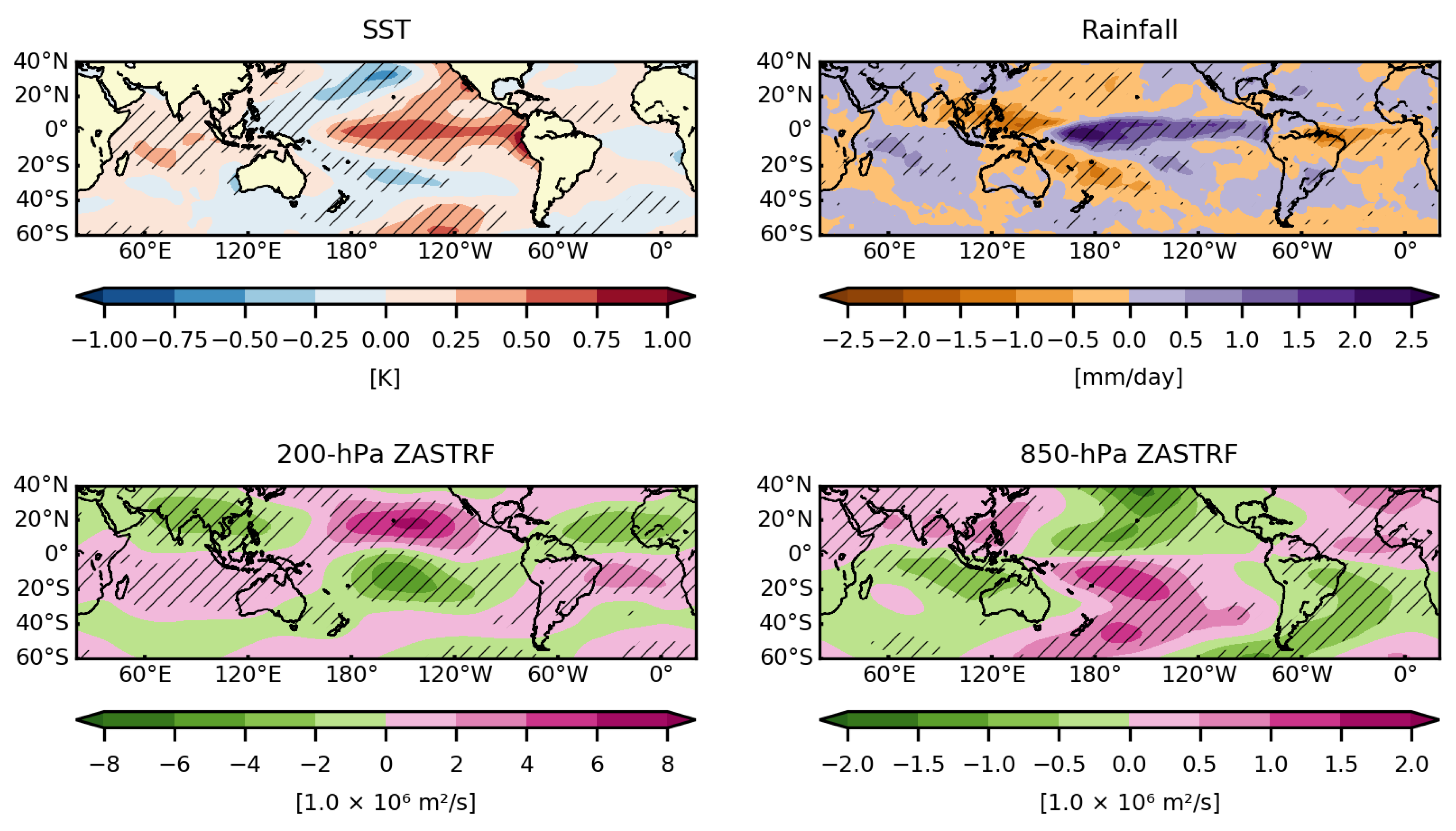
Temporary changes to tropical SST typical patterns, like those that happen during El Niño events, generally induce variations in both the intensity and location of tropical atmospheric convection. These variations, in turn, generate atmospheric circulation anomalies that influence weather and climate all over the globe [77]. SST anomalies in the tropical Pacific strongly influence rainfall conditions in NNEB. Figure 2 shows that anomalous warming (positive SST anomalies) in the central and eastern tropical Pacific (Niño 3.4 region–5° S–5° N/170°–120° W) usually results in increased rainfall in those regions, and reduced rainfall in NNEB. Also related to this anomalous warming are the 200-hPa cyclonic and 850-hPa anticyclonic circulations over NNEB (positive and negative ZASTRF anomalies, respectively), which favour rainfall reduction owing to the descending air motion and reduced thickness associated with upper-level convergence and lower-level divergence in the region—the opposite circulation pattern appears over the central and eastern tropical Pacific. On the other hand, Figure 3 shows that warm SST centred at about 0° × 180°, associated with El Niño Modoki events, generally induces increased rainfall right over it and to the west of it and reduced rainfall along the tropical Pacific, from about 170° W all the way to South America. Reduced rainfall is also observed over NNEB, although with no statistical significance (other studies, e.g., [21], have found statistically significant results when relating El Niño Modoki events to rainfall in NNEB, which may result from the period of analysis and technique employed by the authors). Additionally, 200-hPa and 850-hPa ZASTRF patterns are similar to those shown in Figure 2 but less intense and shifted westward. The 850-hPa circulation over NNEB, however, is not statistically significant in Figure 3. Therefore, circulation patterns related to both canonical and Modoki events induce decreases in rainfall in NNEB, as also shown in [21]. Despite that, the intensity and statistical significance of El Niño Modoki-related atmospheric conditions over NNEB indicate that rainfall anomalies are more likely to deviate from the expected pattern than those related to canonical El Niños (also shown in [28]).
4. Oceanic and Atmospheric Conditions in the 2019 Austral Autumn
4.1. SST and Rainfall Anomalies
In MAM 2019 and the months within that season, El Niño-related warmest waters occurred in the central Pacific, centred at around 165° W (see SST fields in Figure 4). Above-average rainfall was also observed in the central Pacific (Figure 4), with the highest amounts taking place further to the west, at around the International Date Line (180°). In March 2019, positive SST and rainfall anomalies occurred in the tropical South Atlantic and near the southeastern coast of Australia, in the Tasman Sea, whereas the tropical western South Pacific experienced negative rainfall anomalies (the importance of these regions to our study is evidenced later). Negative and positive SST anomalies in the tropical North and South Atlantic Oceans, respectively, suggest that above-average rainfall in NNEB could be associated with the negative phase of AMM. According to NOAA, the normalised AMM SST index, which is the time series of the leading mode of three-month running mean SST and 10 m wind anomalies in the tropical Atlantic [34], was −3.01 in March, −3.54 in April, and −2.08 in May 2019 [78]. This indicates that the AMM most likely contributed to enhancing rainfall in NNEB by disturbing the ITCZ mean position.
Above-average rainfall has been found to take place in NNEB when waters in the Niño 3.4 region are warmer than 0.5° C and deep convection is absent over these waters, as occurred at the initial stages of the 2018–2019 El Niño—this rainfall pattern is, nevertheless, statistically non-significant as found in [79]. If deep convection is present over the Niño 3.4 region warmer-than-normal waters instead, results from [79] show that rainfall in NNEB is significantly below-average (we note that this comment and the previous one are based on composites of monthly precipitation anomalies for the period January 1979–December 2019). The Pacific SST conditions observed in MAM 2019 (Figure 4) resemble those expected during canonical El Niños (Figure 2) more than those seen during Modoki events (Figure 3). The opposite holds for rainfall conditions over the central Pacific. This less usual ocean-atmosphere coupling condition suggests that the 2018–2019 El Niño may then have been an example of a mixed El Niño case (Modoki + canonical [80]).
To further examine the anomalous rainfall pattern in NNEB, we expand our discussion by considering weather station rainfall data measured at seven sites across the region (Figure 1). Moreover, to understand the relative strength of the rainfall anomalies observed in MAM 2019, we compare them to those observed during three strong El Niños—i.e., 1983, 1998, and 2016 [81]. These relatively strong El Niño events supposedly reveal the relationship between El Niños and their associated rainfall anomalies in NNEB more clearly than relatively weak El Niño events, providing a better comprehension to the reader.
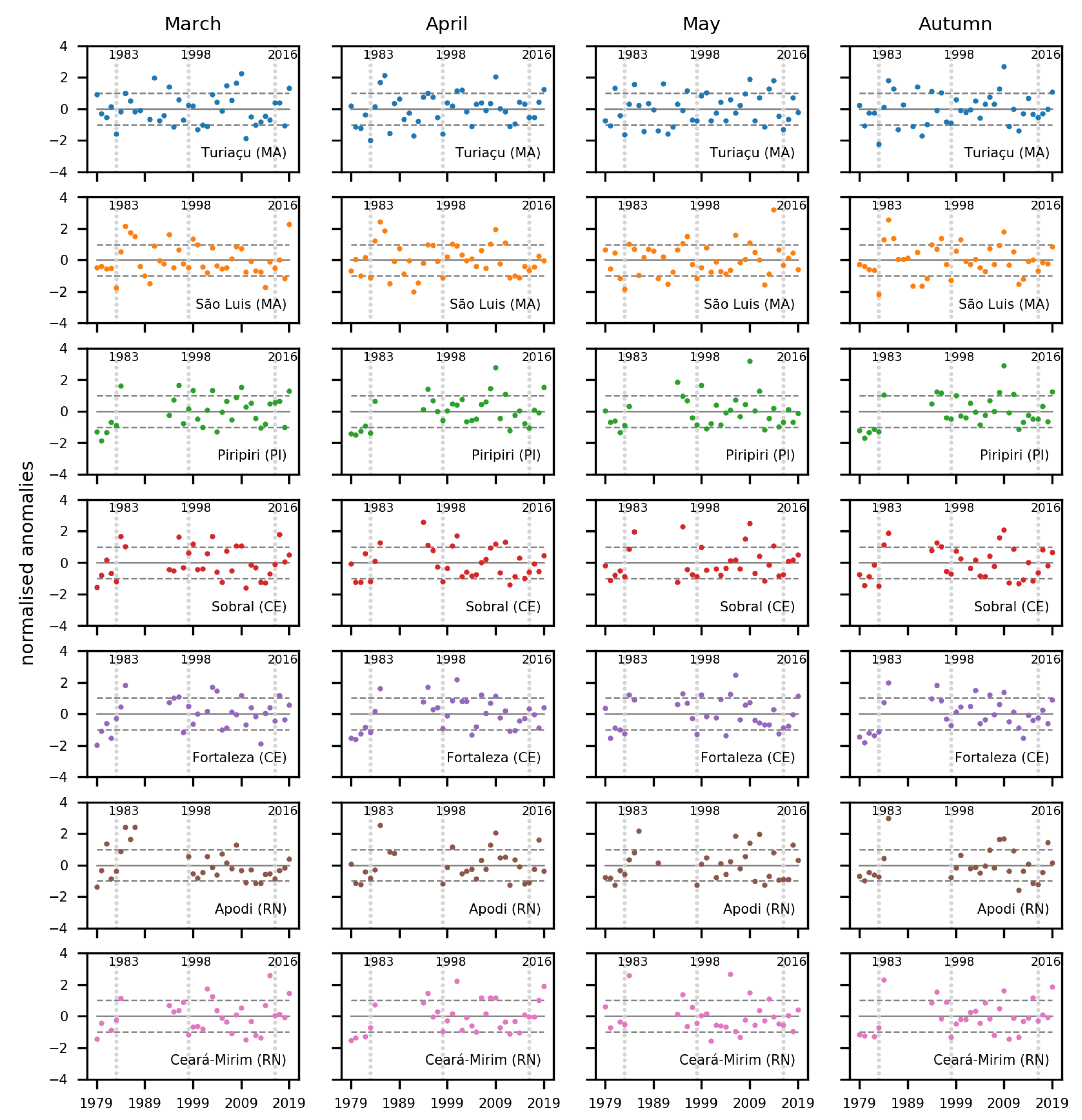
Below-average rainfall in NNEB during El Niño events can be clearly noted in some time series of Figure 5 in years of strong El Niños, such as 1983, 1998, and 2016 (vertical dotted lines). Normalised values lower than −1 standard deviation for the following stations reflects the strength of the anomalies during the 1983 El Niño: Turiaçu and São Luís (March, April, and May), Piripiri (April), Sobral (March and April), and Fortaleza (April and May). These lower-than-normal rainfall values can also be noted for all stations in MAM 1983, except for Apodi and Ceará-Mirim. In 1998, negative rainfall anomalies in NNEB were weaker than in 1983, in general. The easternmost stations (Apodi and Ceará-Mirim) are exceptions. At Apodi station, negative rainfall anomalies were more pronounced in April, May, and MAM 1998 than in the same period in 1983. Rainfall at Ceará-Mirim station behaved similarly, with normalised anomalies more pronounced in March, April, and MAM 1998.
A multi-year drought in NNEB started in 2011 and was aggravated by the 2016 El Niño-related effects. Such drought affected over 30 million people and resulted in more than US$25 billion in economic losses [21]. The weather stations’ data selected here show that the 2016 El Niño was the least associated with below-average rainfall in NNEB, compared to both 1983 and 1998 events. Normalised anomalies for 2016 were negative only at Turiaçu (May), Piripiri (April), and Apodi (April and MAM). The 2016 negative values were more pronounced than those of 1983 (April and MAM) and 1998 (MAM) only at Apodi station, which may be associated, for instance, with local effects or even the Atlantic Multidecadal Oscillation phase change around 1998 [82,83]. A remarkable difference between these three El Niño events is their signature in the Pacific Ocean. Above-average SST featured most prominently in eastern equatorial Pacific waters during the 1983 and 1998 events and in the western and central Pacific during the 2016 El Niño [84].
According to previous studies [79,85], the 2018–2019 El Niño was only weak (weaker east–west SST anomaly gradient across the tropical Pacific than usual El Niños) and characterised by a delayed ocean-atmosphere coupling, i.e., tropical deep atmospheric convection did not shift eastward at the El Niño initial stages despite conducive oceanic conditions. Results from [85] indicate that an anomalous SST gradient between the western and central equatorial Pacific delayed the formation of deep atmospheric convection over the central tropical Pacific and, consequently, of its associated teleconnection patterns. Even though such initial decoupling only lasted from October to December 2018, as stated in [79], NNEB experienced positive rainfall anomalies (above-average rainfall) in MAM 2019 (Figure 4 and Figure 5), which contrasts the negative rainfall anomalies (below-average rainfall) typically observed in the region during El Niño episodes (Figure 2 and Figure 3). Positive rainfall anomalies were observed at all seven stations in March 2019, with, in particular, normalised values exceeding one standard deviation at four of them (Turiaçu, São Luís, Piripiri, and Ceará-Mirim). In April 2019, the most pronounced above-average rainfall took place at three out of the seven stations analysed (Turiaçu, Piripiri, and Ceará-Mirim). Fortaleza was the only station that experienced positive rainfall anomalies above one standard deviation in May 2019. In MAM 2019, positive anomalies were remarkably stronger at three stations (Turiaçu, Piripiri, and Ceará-Mirim) compared to other sites. There was no below-normal rainfall in March and MAM 2019.
In 2019, São Luís, Ceará-Mirim, and Piripiri stations recorded not only above-average rainfall but some of the highest rainfall values of the last 40 years (Figure 5). At São Luís station, rainfall in March 2019 was the highest on record (1979–2019) for March months, with a normalised anomaly value of ~2.3 standard deviations. Additionally, in March 2019, Ceará-Mirim station experienced the third-highest March rainfall since 1979 (~1.5 standard deviations). Rainfall amounts at Ceará-Mirim station in April and MAM 2019 were the second-highest relative to corresponding periods in previous years (~1.9 standard deviations in both cases). In 2019, Piripiri station recorded the second-and third-highest rainfall amounts for April and MAM, respectively, when considering the period 1979–2019 (~1.6 and ~1.3 standard deviations for April and MAM, respectively).
The previous four paragraphs highlight the month-to-month rainfall amount differences for data recorded at individual weather stations during an El Niño event. In addition to the contribution of the negative phase of AMM, the aforementioned month-to-month differences also suggest a contribution of sub-seasonal oscillations (e.g., the MJO) to rainfall variability in NNEB, which can disturb El Niño-related impacts (addressed later in Section 6).
4.2. Atmospheric Circulation Anomalies
The ocean-atmosphere coupling during MAM 2019 triggered circulation conditions over NNEB (Figure 6) that differ from those expected during El Niño events (Figure 2 and Figure 3). An upper-level (200 hPa) Rossby wave train connected the South Pacific to the tropical South Atlantic through the extratropics (more notable in MAM and March 2019), resulting in an anticyclonic circulation over the tropical South Atlantic and part of eastern South America (Figure 6). This anticyclonic circulation likely caused upper-level divergence over NNEB, favouring above-average rainfall occurrence in the region, unlike the typically observed below-average rainfall conditions associated with El Niño-related cyclonic circulations (Figure 2 and Figure 3). In the lower troposphere (850 hPa), the circulation also opposed the El Niño-related usual conditions, with a cyclonic circulation appearing over part of NNEB, except in May and MAM 2019 (Figure 6).
5. Model Results
5.1. Influence Functions
The impacts of diabatic heating anomalies on circulation were assessed at five TPs (Figure 7–the TPs can also be seen in the March panels of Figure 6). The selection of TPs 1–4 aimed to understand the origin of the teleconnection pattern that connected the extratropical South Pacific to the tropical South Atlantic. More specifically, we chose the first four TPs because the 200-hPa anticyclonic circulation in March 2019 over the tropical South Atlantic seems connected to the circulation pattern upstream (Figure 6), resembling, therefore, the Pacific-South American teleconnection associated with ENSO and the MJO, as well as modulation of rainfall variability in tropical South America at seasonal and sub-seasonal timescales [86]. TP5 was selected to identify potential TFs influencing the local circulation over NNEB.
The IFs results for TPs 1–4 (Figure 7) indicate that circulation anomalies associated with the teleconnection pattern observed in the reanalysis data (Figure 6–March panels) were likely triggered by TFs over the western South Pacific—this is shown by the sign reversal of IFs results as TP locations vary (Figure 7). Although TFs over other regions (e.g., central South Pacific) may seem to influence circulation around TPs strongly, the signs of IFs results do not reverse as TP locations change. The absence of such a sign reversal results in conflicting influences at the TPs, as highlighted by [58]. The IFs results for TPs 1 and 2 show that the dipole-like rainfall pattern observed in the GPCP data, with negative anomalies (cooling) at ~12° S/160° E and positive anomalies (heating) at ~35° S/160° E (Figure 4–March panel), may trigger a barotropic circulation around these TPs (Figure 7) as the one observed in the reanalysis data (Figure 6–March panels). TFs over the western South Pacific, especially near the eastern/southeastern coast of Australia (over the Tasman Sea), may also modulate circulation anomalies around TP3. 850-hPa and 200-hPa IFs results show opposite signs over the western subtropical South Pacific (Figure 7), indicating that the “quasi-baroclinic” circulation around TP3 (Figure 6–March panels) was likely induced by heating anomalies over the Tasman Sea (see March rainfall field in Figure 4).
To obtain the 200-hPa anticyclonic circulation and 850-hPa cyclonic circulation around TP4, as observed in Figure 6 (March panels), the IFs results point out that cooling anomalies over most parts of the Pacific Ocean and Australia are necessary. Because IF results over the western South Pacific all have signs of the same polarity for TP4, the effects of the dipole-like rainfall pattern on TP4 are likely smoothed. This is because the same sign polarity indicates conflicting influences, in this case, showing that the teleconnection pattern action centres around TPs 1–4 are not equally excited by the dipole-like rainfall pattern. The IFs fields for TP4 also show that the local effects associated with heating anomalies over the tropical South Atlantic (March panel in Figure 4) contribute to modulating the baroclinic circulation observed in the reanalysis data (Figure 6–March panels). Regarding the effects of TFs on circulation around TP5, the IFs indicate that heating anomalies associated with above-average rainfall in the western-central equatorial Pacific likely modulate circulation anomalies over the region near NNEB (Figure 7). Local TFs associated with deep diabatic heating anomalies, on the other hand, do not seem to affect the local circulation. This is indicated by opposite 850-hPa and 200-hPa IFs results over NNEB and adjacent equatorial Atlantic, which contrast those observed in reanalysis data (Figure 6–March panels).
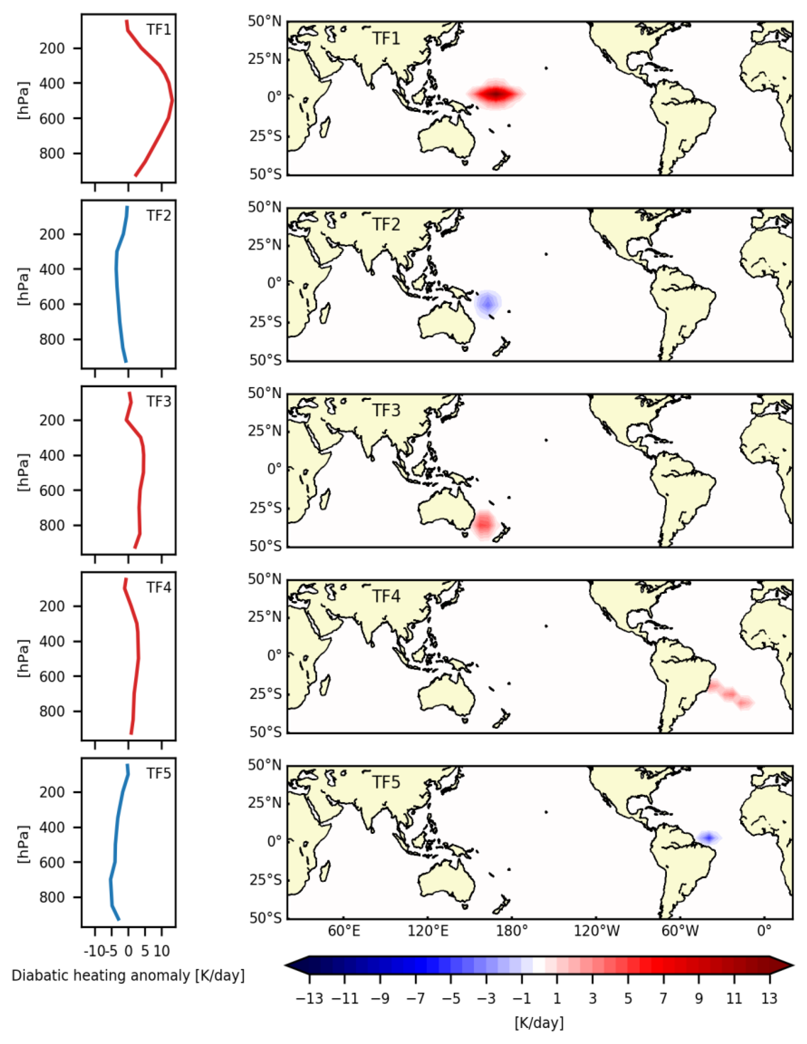
The IFs results (Figure 7), along with the GPCP rainfall data (Figure 4–March panel), suggest that deep diabatic heating anomalies in four regions may have contributed the most to above-normal rainfall in NNEB in March 2019. These regions comprise the following areas (TFs 1–4 in Table 1): ~5° S–7.5° N/150° E–170° W (TF1); ~20°–5° S/155°–170° E (TF2); ~40°–25° S/152°–168° E (TF3); and ~35°–15° S/43°–10° W (TF4). The way this hypothesis was tested is explained next.
Figure 7.
Influence functions (IFs) results for five target points (TP1–TP5–black dots), considering the March climatological basic state. IFs were applied to modelled 200-hPa (left panels) and 850-hPa (right panels) zonally asymmetric stream function (ZASTRF) anomalies, for thermal forcings between 35° S and 35° N (straight horizontal lines), on the 15th day of simulation. Magenta (green) contours (1 × 10⁶ m2/s) indicate positive (negative) ZASTRF anomalies around the TP for positive diabatic heating anomalies. Dashed lines indicate zero contours.

5.2. Vertical and Horizontal Distributions of Thermal Forcings
The vertical and horizontal distributions of TFs 1–4, incorporated into the model’s temperature tendency equation, are shown in Figure 8. According to Table 1, their respective peaks are 13.1 K day−1 (at 500 hPa), −3.6 K day−1 (at 400 hPa), 4.6 K day−1 (at 400 hPa), and 3.1 K day−1 (at 500 hPa). We considered, in addition, two forcing nodes peaking in the lower troposphere (700 hPa and 850 hPa). One of the nodes (−5.3 K day−1 at 700 hPa–TF5) relates to negative rainfall anomalies to the north of NNEB; its associated area comprises ~2.5° S–7.5° N/48°–32° W (Figure 8 and Table 1). The other one relates to positive rainfall anomalies over the entire equatorial Atlantic and is associated with the ITCZ cloud band (not shown). As shown later, the 850-hPa ZASTRF response over the tropical South Atlantic slightly improves when considering TF5 (shallow cooling anomalies). In contrast, the simulations that considered shallow heating anomalies over the entire equatorial Atlantic did not provide additional insights into the modulation of atmospheric circulations associated with the above-normal rainfall in NNEB (not shown). Therefore, we will not discuss the latter simulation.
5.3. Modelled ZASTRF Anomalies
To confirm the IFs results and, thus, assess the origin of the atmospheric circulation anomalies that most contributed to above-normal rainfall in NNEB in March 2019, we carried out a set of model experiments that considered the following combinations among the different TFs (diabatic heating anomalies–Figure 8): (i) TFs 2 and 3; (ii) TFs 2–4; (iii) TFs 1–4; and (iv) TFs 1–5. Because the dynamical framework within the LBM employed is simplified, we only focused on the qualitative aspect of the model results (Figure 9).
The dipole-like TF over the western South Pacific (TF2 + TF3 in Figure 8) generated a teleconnection pattern that connects the extratropical South Pacific to South Atlantic (TF2 + TF3 in Figure 9). These circulation anomalies have a barotropic structure over the central-southeastern South Pacific and a baroclinic structure over the South America–South Atlantic sector. Experiments using TF2 and TF3 separately showed that TF2 generated circulation anomalies over the South Atlantic through tropical wave dispersion, whilst TF3 triggered extratropical circulation anomalies (not shown). By combining TF4 with TF2 and TF3, results improve and show a baroclinic circulation over the South Atlantic (TF2 + TF3 + TF4 in Figure 9) that more closely resembles the one observed in the reanalysis data (compared to March panels of Figure 6—note that colour scales are different to allow better visualisation). Such improvement indicates that this baroclinic circulation is modulated by enhanced rainfall (more condensation heating–TF4 in Figure 8) in the tropical South Atlantic, which, in turn, is likely caused by the warmer-than-normal SST underneath (Figure 4). The inclusion of TF1 as the fourth model forcing generates upper-level (200 hPa) positive ZASTRF anomalies to the north of NNEB (TF1 + TF2 + TF3 + TF4 in Figure 9), as seen in the reanalysis data (Figure 6).
When used as the only model forcing, TF1 (diabatic heating anomalies over the equatorial Pacific–Figure 8) induces a baroclinic circulation over the tropical South Atlantic (cyclonic at 200 hPa and anticyclonic at 850 hPa (not shown)). This circulation pattern contrasts with the one observed in the reanalysis data (Figure 6). By considering the five TFs together, the lower-level circulation (850 hPa) over the equatorial Atlantic improves slightly (TF1 + TF2 + TF3 + TF4 + TF5 in Figure 9), resembling the one seen in the reanalysis data a bit more (Figure 6). Therefore, this set of experiments suggests that remote and local forcings jointly modulated the circulation anomalies that resulted in above-normal rainfall in NNEB, as indicated by the IFs results.
6. MJO Contributions to the MAM 2019 Rainfall in NNEB
To further explore mechanisms that may have led to the above-normal rainfall in NNEB in MAM 2019, we examined MJO-related conditions in that period. Figure 10 shows the RMM diagram [75] for March, April, and May 2019. MJO phases 2 and 3 occurred in the first five days of March and the period 20–27 April. These MJO phases increase the chances of above-average rainfall in NNEB [87]—we note that the effects associated with a given MJO phase may last up to about ten days after this phase ends [67,88], which likely prolonged the influence of the effects related to MJO phases 2 and 3 on rainfall in NNEB in March 2019. In fact, March was the wettest month of MAM 2019 in NNEB, with ~60% of the weather stations analysed presenting above-average rainfall (Figure 5). In April 2019, above-average rainfall occurred at ~40% of the stations. MJO-related convection locates in more northern latitudes from April to September [89], accompanying the ITCZ cloud band displacement. This may have contributed to decreasing the number of stations that recorded positive rainfall anomalies in April 2019 relative to the previous month. Although MJO phase 2 took place in the last two days of May 2019, MJO-related convection does not seem to have influenced rainfall in NNEB substantially in that month.
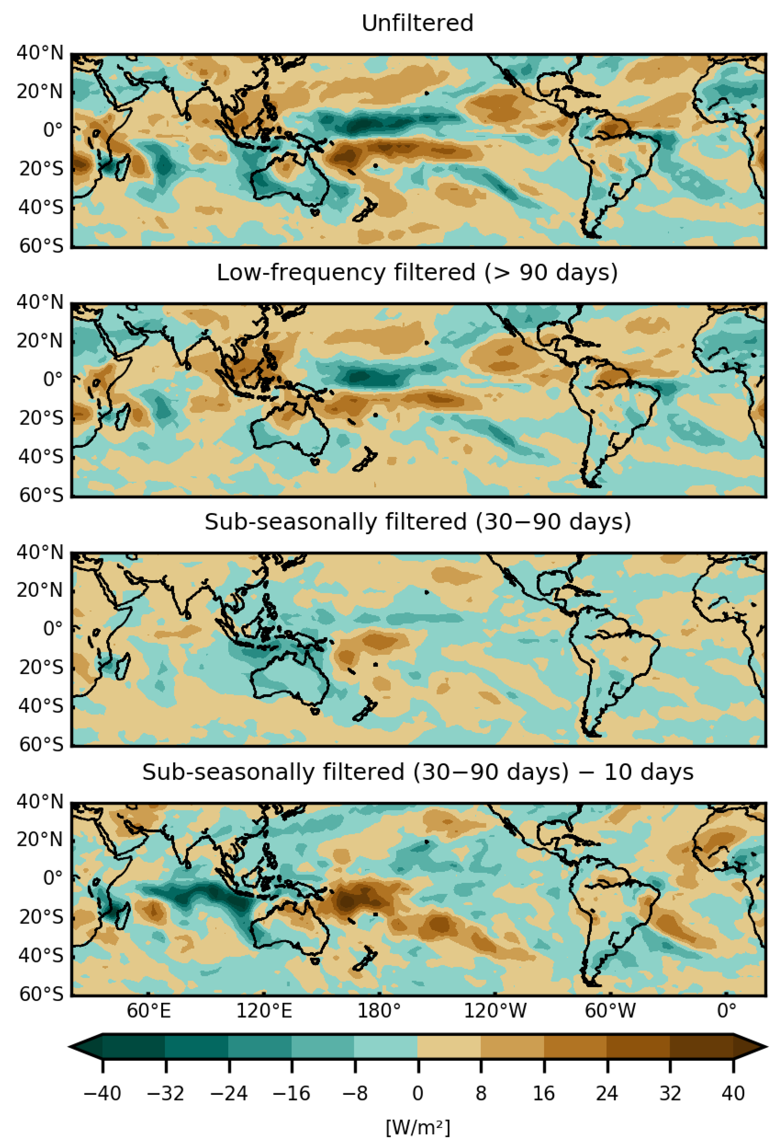
As MJO-related convection seems to have played a more decisive role in NNEB rainfall amounts in March 2019, in comparison to the subsequent two months, we now focus on that month and analyze OLR anomalies filtered at different timescales. Low-frequency signals (>90 days) by themselves do not explain all unfiltered OLR anomalies (Figure 11), suggesting a contribution of oscillations at other timescales to the modulation of atmospheric convection processes.
Sub-seasonal signals (30–90 days) for March 2019 indicate reduced convection over NNEB, on average, except right over part of the NNEB coastline. Positive and negative OLR anomalies over the western South Pacific at this timescale seem to reinforce low-frequency anomalies over that area. This reinforcement results in anomalous 200-hPa and 850-hPa circulation conditions that favour the formation of an anticyclone and a cyclone, respectively, over tropical South America and adjacent South Atlantic, as found in the model response to TF2+TF3 (Figure 9). As a consequence, such circulation conditions may favour anomalous rainfall occurrence in NNEB, as previously stated. In opposition to monthly averaged sub-seasonal signals (30–90 days), those averaged over the first ten days of March 2019 indicate that convection was taking place over NNEB. This indicates that these days were, therefore, the period in which sub-seasonal OLR anomalies over NNEB contributed to strengthening low-frequency signals, which resulted in above-normal rainfall in that region. Thus, MJO-related sub-seasonal signals very likely contributed to modulating deep atmospheric convection anomalies over the western South Pacific during March, as a whole, and to developing convection over NNEB during the first ten days of the month.
7. Conclusions
Understanding the differences between rainfall conditions during El Niño events is essential to water resources management, agriculture, livestock, and the safety of people and infrastructure. In 2019, NNEB experienced above-average rainfall in austral autumn, contrasting the below-normal rainfall conditions that typically take place during El Niños. To investigate this rainfall anomaly, we analysed atmospheric and oceanic conditions using several datasets, which allowed us to realise that above-normal rainfall in NNEB in autumn 2019 was likely associated with four main combined factors; these are (1) the weak intensity of the 2019 El Niño (as stated by [79,85]); (2) the negative phase of AMM; (3) local and remote diabatic heating anomalies, especially over the western South Pacific and tropical South Atlantic; and (4) MJO activity during the first ten days of March 2019.
As reported in previous work, the 2019 El Niño was only weak and associated with an anomalous SST gradient between the western and central equatorial Pacific waters [85]. Such a gradient delayed the El Niño-related ocean-atmosphere coupling development [85], contributing to different impacts in remote areas from those expected during these events. In certain regions, such as NNEB, atmospheric conditions behaved oppositely to those generally observed during El Niños. Concurrent diabatic heating anomalies over several regions during March 2019 resulted in anticyclonic and cyclonic circulations in the upper and lower troposphere, respectively, over the tropical South Atlantic that induced ascending motion over NNEB. Deep cooling anomalies (negative rainfall anomalies) were observed over the tropical western South Pacific, whereas deep heating anomalies (positive rainfall anomalies) occurred near the eastern/southeastern coast of Australia (over the Tasman Sea). Local effects resulted mainly from deep heating anomalies over the tropical South Atlantic. Two more TFs contributed to the circulation that affected rainfall over NNEB in March 2019. Deep heating anomalies over the equatorial Pacific influenced mostly the upper-level (200 hPa) circulation over the seaward area to the north of NNEB, whilst shallow cooling anomalies over the equatorial Atlantic, to the north of NNEB, impacted chiefly the lower-level (850 hPa) circulation over the tropical South Atlantic. All these anomalous TFs combined generated circulation anomalies that caused above-average rainfall in NNEB. MJO phases 2 and 3 coincided with sub-seasonal oscillations that intensified low-frequency atmospheric convection anomalies over the western South Pacific in March 2019 and over NNEB during the first ten days of the month, suggesting, therefore, an influence of MJO-related atmospheric convection on NNEB rainfall in that period.
Daily rainfall data may help elucidate how MJO activity contributed to rainfall in NNEB in autumn 2019. For instance, ~39% of the March 2019 accumulated rainfall at São Luís station (321.6 mm, out of 818.2 mm) occurred during the first ten days of the month (not shown), when MJO phases were favourable to increased rainfall in the region. This rainfall amount, summed to that of an isolated weather event on 24 March 2019 (234.4 mm), totalises ~68% of the accumulated rainfall in that month (556.0 mm). Relationships between rainfall in NNEB and other weather phenomena such as eastern wave disturbances, upper-level cyclonic vortices, mesoscale convective systems, and squall lines during the period analysed here are also worthy of investigation, given that previous studies have found a significant association between them [90,91]. A more complex numeric model than the one we employed here, which allows for using SST fields as boundary conditions and, therefore, provides more realistic atmospheric responses [92], may, for instance, assist in assessing the influence of AMM-related tropical Atlantic SST anomalies on the modulation of mesoscale convective systems in March 2019. The intensification of these systems embedded in the ITCZ likely contributed to inducing above-average rainfall in NNEB. Nevertheless, our results complement findings of the previous studies that characterised less common El Niño events (e.g., [79,85,93]), marked by ocean-atmosphere decoupling at initial stages, such as those that occurred in 1979–1980, 2004–2005, 2014–2015, and 2018–2019 [79]. Our results also support the conclusion by [79] that states that El Niño-related rainfall anomalies cannot be predicted accurately based solely on SST anomalies in the tropical Pacific. Atmosphere-ocean coupling is crucial to trigger remote rainfall anomalies. Even when the coupling takes place, like during the period analysed here, rainfall anomalies may not follow the expected pattern for El Niño. This rainfall pattern has been reported here, reinforcing how much ENSO-related anomalies matter to rainfall occurrence and intensity in NNEB. Besides the ENSO’s phase (El Niño or La Niña) and flavour (canonical or Modoki), the intensity of its associated anomalies is of paramount importance to determine whether below-normal or above-normal rainfall should be expected in NNEB.
Author Contributions
Conceptualization, F.M.d.A. and V.A.G.; data curation, F.M.d.A. and V.A.G.; formal analysis, F.M.d.A., V.A.G. and J.A.A.; investigation, F.M.d.A. and V.A.G.; methodology, F.M.d.A., V.A.G. and J.A.A.; validation, F.M.d.A., V.A.G. and J.A.A.; visualization, F.M.d.A., V.A.G. and J.A.A.; writing—original draft, F.M.d.A. and V.A.G.; writing—review and editing, F.M.d.A., V.A.G. and J.A.A. All authors have read and agreed to the published version of the manuscript.
Funding
This research received no external funding.
Data Availability Statement
The data and material used in this research can be found at the following websites: www.inmet.gov.br, https://apps.ecmwf.int/datasets/data/interim-full-moda/levtype=sfc/, https://psl.noaa.gov/data/gridded/data.noaa.ersst.v5.html, https://psl.noaa.gov/data/gridded/data.interp_OLR.html, https://psl.noaa.gov/data/gridded/data.gpcp.html, https://ccsr.aori.u-tokyo.ac.jp/~lbm/sub/lbm.html. The Python codes used in this research are available upon request from the first author.
Acknowledgments
The authors are thankful to INMET (www.inmet.gov.br), ECMWF (https://apps.ecmwf.int/datasets/data/interim-full-moda/levtype=sfc/), NOAA (https://psl.noaa.gov/data/gridded/data.noaa.ersst.v5.html, https://psl.noaa.gov/data/gridded/data.gpcp.html, and https://psl.noaa.gov/data/gridded/data.interp_OLR.html) for providing the data employed in this research. We also thank Steven Woolnough for providing the code to plot the RMM diagram and Michiya Hayashi and Masahiro Watanabe for providing the LBM code (https://ccsr.aori.u-tokyo.ac.jp/~lbm/sub/lbm.html).
Conflicts of Interest
The authors declare no conflict of interest.
References
- Wallace, J.M.; Hobbs, P.V.; McMurdie, L.; Houze, R.A. Weather Systems. In Atmospheric Science—An Introductory Survey, 2nd ed.; Elsevier: Amsterdam, The Netherlands, 2006; pp. 313–373. [Google Scholar] [CrossRef]
- Houze, R.A. Cumulonimbus and Severe Storms. Cloud Dyn. 2014, 104, 187–236. [Google Scholar] [CrossRef]
- Mantua, N.J.; Hare, S.R. The Pacific Decadal Oscillation. J. Oceanogr. 2002, 58, 35–44. [Google Scholar] [CrossRef]
- Walker, G.T.; Bliss, E.W. World Weather V. Mem. R. Meteorol. Soc. 1932, 4, 53–84. [Google Scholar] [CrossRef]
- Walker, G.T.; Bliss, E.W. World Weather V. Mem. R. Meteorol. Soc. 1937, 4, 119–139. [Google Scholar] [CrossRef]
- Bjerknes, J. “El Niño” study based on analysis of ocean surface temperatures 1935–1957. Inter. Am. Trop. Tuna Comm. Bull. 1961, 5, 217–303. [Google Scholar]
- Bjerknes, J. A possible response of the atmospheric Hadley circulation to equatorial anomalies of ocean temperature. Tellus 1966, 18, 820–829. [Google Scholar] [CrossRef] [Green Version]
- Wyrtki, K. El Niño—The dynamic response of the equatorial Pacific Ocean to atmospheric forcing. J. Phys. Oceanogr. 1975, 5, 572–584. [Google Scholar] [CrossRef]
- Neelin, J.D.; Battisti, D.S.; Hirst, A.C.; Jin, F.-F.; Wakata, Y.; Yamagata, T.; Zebiak, S.E. ENSO theory. J. Geophys. Res. Oceans 1998, 103, 14261–14290. [Google Scholar] [CrossRef] [Green Version]
- Trenberth, K.E.; Hurrell, J.W. Decadal atmosphere-ocean variations in the Pacific. Clim. Dyn. 1994, 9, 303–319. [Google Scholar] [CrossRef]
- Cane, M.A. The evolution of El Niño, past and future. Earth Planet. Sci. Lett. 2005, 230, 227–240. [Google Scholar] [CrossRef]
- McPhaden, M.J.; Zebiak, S.E.; Glantz, M.H. ENSO as an Integrating Concept in Earth Science. Science 2006, 314, 1740–1745. [Google Scholar] [CrossRef] [Green Version]
- Chase, T.N.; Pielke Sr, R.A.; Avissa, R. Teleconnections in the Earth System. In Encyclopedia of Hydrological Sciences; Anderson, M.G., Ed.; Wiley: Hoboken, NJ, USA, 2006. [Google Scholar] [CrossRef]
- Lin, J.; Qian, T. A New Picture of the Global Impacts of El Nino-Southern Oscillation. Sci. Rep. 2019, 9, 17543. [Google Scholar] [CrossRef] [Green Version]
- Nicholls, N. Towards the prediction of major Australian droughts. Aust. Met. Mag. 1985, 33, 161–166. [Google Scholar]
- Nicholls, N. The El Niño/Southern Oscillation and Australian vegetation. Plant Ecol. 1991, 91, 23–36. [Google Scholar] [CrossRef]
- Cai, W.; Cowan, T. Dynamics of late autumn rainfall reduction over southeastern Australia. Geophys. Res. Lett. 2008, 35, L09708. [Google Scholar] [CrossRef]
- Taschetto, A.S.; England, M.H. El Niño Modoki Impacts on Australian Rainfall. J. Clim. 2009, 22, 3167–3174. [Google Scholar] [CrossRef] [Green Version]
- Cai, W.; van Rensch, P.; Cowan, T.; Hendon, H.H. Teleconnection Pathways of ENSO and the IOD and the Mechanisms for Impacts on Australian Rainfall. J. Clim. 2011, 24, 3910–3923. [Google Scholar] [CrossRef]
- Davey, M.; Brookshaw, A.; Ineson, S. The probability of the impact of ENSO on precipitation and near-surface temperature. Clim. Risk Manag. 2014, 1, 5–24. [Google Scholar] [CrossRef] [Green Version]
- Cai, W.; McPhaden, M.J.; Grimm, A.M.; Rodrigues, R.R.; Taschetto, A.S.; Garreaud, R.D.; Dewitte, B.; Poveda, G.; Ham, Y.-G.; Santoso, A.; et al. Climate impacts of the El Niño–Southern Oscillation on South America. Nat. Rev. Earth Environ. 2020, 1, 215–231. [Google Scholar] [CrossRef]
- Grimm, A.M.; Ambrizzi, T. Teleconnections into South America from the tropics and extratropics on interannual and intraseasonal timescales. In Past Climate Variability in South America and Surrounding Regions; Vimeux, F., Sylvestre, F., Khodri, M., Eds.; Developments in Paleoenvironmental Research; Springer: Dordrecht, The Netherland, 2009; pp. 159–191. [Google Scholar] [CrossRef]
- Stan, C.; Straus, D.M.; Frederiksen, J.S.; Lin, H.; Maloney, E.D.; Schumacher, C. Review of Tropical-Extratropical Teleconnections on Intraseasonal Time Scales. Rev. Geophys. 2017, 55, 902–937. [Google Scholar] [CrossRef]
- Shimizu, M.H.; de Albuquerque Cavalcanti, I.F. Variability patterns of Rossby wave source. Clim. Dyn. 2011, 37, 441–454. [Google Scholar] [CrossRef]
- L’heureux, M.L.; Thompson, D.W.J. Observed Relationships between the El Niño–Southern Oscillation and the Extratropical Zonal-Mean Circulation. J. Clim. 2006, 19, 276–287. [Google Scholar] [CrossRef] [Green Version]
- Grimm, A.M. Interannual climate variability in South America: Impacts on seasonal precipitation, extreme events, and possible effects of climate change. Stoch. Environ. Res. Risk Assess. 2011, 25, 537–554. [Google Scholar] [CrossRef]
- Tedeschi, R.G.; Grimm, A.M.; Cavalcanti, I.F.A. Influence of Central and East ENSO on extreme events of precipitation in South America during austral spring and summer. Int. J. Clim. 2015, 35, 2045–2064. [Google Scholar] [CrossRef]
- Tedeschi, R.G.; Grimm, A.M.; Cavalcanti, I.F.A. Influence of Central and East ENSO on precipitation and its extreme events in South America during austral autumn and winter. Int. J. Clim. 2016, 36, 4797–4814. [Google Scholar] [CrossRef]
- Saravanan, R.; Chang, P. Interaction between tropical Atlantic variability and El Niño–Southern Oscillation. J. Clim. 2000, 13, 2177–2194. [Google Scholar] [CrossRef]
- Hastenrath, S. Circulation and teleconnection mechanisms of Northeast Brazil droughts. Prog. Oceanogr. 2006, 70, 407–415. [Google Scholar] [CrossRef]
- Rodrigues, R.R.; Haarsma, R.J.; Campos, E.J.D.; Ambrizzi, T. The Impacts of Inter–El Niño Variability on the Tropical Atlantic and Northeast Brazil Climate. J. Clim. 2011, 24, 3402–3422. [Google Scholar] [CrossRef] [Green Version]
- Lucena, D.B.; Servain, J.; Filho, M.F.G. Rainfall Response in Northeast Brazil from Ocean Climate Variability during the Second Half of the Twentieth Century. J. Clim. 2011, 24, 6174–6184. [Google Scholar] [CrossRef]
- Hastenrath, S.; Greischar, L. Circulation mechanisms related to northeast Brazil rainfall anomalies. J. Geophys. Res. Atmos. 1993, 98, 5093–5102. [Google Scholar] [CrossRef]
- Chiang, J.C.H.; Vimont, D.J. Analogous Pacific and Atlantic Meridional Modes of Tropical Atmosphere–Ocean Variability in the tropical Pacific and tropical Atlantic. J. Clim. 2004, 17, 4143–4158. [Google Scholar] [CrossRef]
- Wagner, R.G. Mechanisms Controlling Variability of the Interhemispheric Sea Surface Temperature Gradient in the Tropical Atlantic. J. Clim. 1996, 9, 2010–2019. [Google Scholar] [CrossRef]
- Chang, P.; Ji, L.; Li, H. A decadal climate variation in the tropical Atlantic Ocean from thermodynamic air-sea interactions. Nature 1997, 385, 516–518. [Google Scholar] [CrossRef]
- Goddard, L.; Aitchellouche, Y.; Baethgen, W.; Dettinger, M.; Graham, R.; Hayman, P.; Kadi, M.; Martínez, R.; Meinke, H. Providing Seasonal-to-Interannual Climate Information for Risk Management and Decision-making. Procedia Environ. Sci. 2010, 1, 81–101. [Google Scholar] [CrossRef] [Green Version]
- Creedy, T.J.; Asare, R.A.; Morel, A.C.; Hirons, M.; Mason, J.; Malhi, Y.; McDermott, C.L.; Opoku, E.; Norris, K. Climate change alters impacts of extreme climate events on a tropical perennial tree crop. Sci. Rep. 2022, 12, 19653. [Google Scholar] [CrossRef]
- Nobre, G.G.; Muis, S.; Veldkamp, T.I.; Ward, P.J. Achieving the reduction of disaster risk by better predicting impacts of El Niño and La Niña. Prog. Disaster Sci. 2019, 2, 100022. [Google Scholar] [CrossRef]
- Giovannettone, J.; Paredes, F.; Barbosa, H.; Dos Santos, C.A.C.; Kumar, T.V.L. Characterization of links between hydro-climate indices and long-term precipitation in Brazil using correlation analysis. Int. J. Clim. 2020, 40, 5527–5541. [Google Scholar] [CrossRef]
- Valadão, C.E.A.; Carvalho, L.M.V.; Lucio, P.S.; Chaves, R.R. Impacts of the Madden-Julian oscillation on intraseasonal precipitation over Northeast Brazil. Int. J. Clim. 2016, 37, 1859–1884. [Google Scholar] [CrossRef]
- Junior, F.D.C.V.; Jones, C.; Gandu, A.W.; Martins, E.S.P.R. Impacts of the Madden-Julian Oscillation on the intensity and spatial extent of heavy precipitation events in northern Northeast Brazil. Int. J. Clim. 2021, 41, 3628–3639. [Google Scholar] [CrossRef]
- Mo, K.C.; Nogues-Paegle, J. Pan-America. In Intraseasonal Variability in the Atmosphere-Ocean Climate System; Springer Praxis Books (Environmental Sciences); Springer: Berlin/Heidelberg, Germany, 2005; pp. 95–124. [Google Scholar] [CrossRef]
- Shimizu, M.H.; Ambrizzi, T. MJO influence on ENSO effects in precipitation and temperature over South America. Theor. Appl. Clim. 2015, 124, 291–301. [Google Scholar] [CrossRef]
- Shimizu, M.H.; Ambrizzi, T.; Liebmann, B. Extreme precipitation events and their relationship with ENSO and MJO phases over northern South America. Int. J. Climatol. 2017, 37, 2977–2989. [Google Scholar] [CrossRef]
- Dee, D.P.; Uppala, S.M.; Simmons, A.J.; Berrisford, P.; Poli, P.; Kobayashi, S.; Andrae, U.; Balmaseda, M.A.; Balsamo, G.; Bauer, P.; et al. The ERA-Interim reanalysis: Configuration and performance of the data assimilation system. Q. J. R. Meteorol. Soc. 2011, 137, 553–597. [Google Scholar] [CrossRef]
- Nichols, G.P.; Fontenot, J.D.; Gibbons, J.P.; Sanders, M. Evaluation of volumetric modulated Arc therapy for postmastectomy treatment. Radiat. Oncol. 2017, 30, 8179–8205. [Google Scholar] [CrossRef] [PubMed] [Green Version]
- Adler, R.F.; Sapiano, M.R.P.; Huffman, G.J.; Wang, J.-J.; Gu, G.; Bolvin, D.; Chiu, L.; Schneider, U.; Becker, A.; Nelkin, E.; et al. The Global Precipitation Climatology Project (GPCP) Monthly Analysis (New Version 2.3) and a Review of 2017 Global Precipitation. Atmosphere 2018, 9, 138. [Google Scholar] [CrossRef] [PubMed] [Green Version]
- Liebmann, B.; Smith, C.A. Description of a complete (interpolated) outgoing longwave radiation dataset. Bull. Am. Meteorol. Soc. 1996, 77, 1275–1277. [Google Scholar]
- Junker, N.W.; Grumm, R.H.; Hart, R.; Bosart, L.F.; Bell, K.M.; Pereira, F.J. Use of Normalized Anomaly Fields to Anticipate Extreme Rainfall in the Mountains of Northern California. Weather. Forecast. 2008, 23, 336–356. [Google Scholar] [CrossRef] [Green Version]
- Allen, M.P. The t test for the simple regression coefficient. In Understanding Regression Analysis; Springer: Boston, MA, USA, 1997; pp. 66–70. [Google Scholar] [CrossRef]
- Trenberth, K.E. The definition of el nino. Bull. Am. Meteorol. Soc. 1997, 78, 2771–2778. [Google Scholar] [CrossRef]
- Trenberth, K.E.; Stepaniak, D.P. Indices of El Niño evolution. J. Clim. 2001, 14, 1697–1701. [Google Scholar] [CrossRef]
- Ashok, K.; Behera, S.K.; Rao, S.A.; Weng, H.; Yamagata, T. El Niño Modoki and its possible teleconnection. J. Geophys. Res. Ocean. 2007, 112, C11007. [Google Scholar] [CrossRef]
- Lo, F.; Hendon, H.H. Empirical Extended-Range Prediction of the Madden–Julian Oscillation. Mon. Weather. Rev. 2000, 128, 2528–2543. [Google Scholar] [CrossRef]
- Livezey, R.E.; Chen, W.Y. Statistical field significance and its determination by Monte Carlo techniques. Mon. Wea. Rev. 1983, 111, 46–59. [Google Scholar] [CrossRef]
- Branstator, G. Analysis of General Circulation Model Sea-Surface Temperature Anomaly Simulations Using a Linear Model. Part I: Forced Solutions. J. Atmos. Sci. 1985, 42, 2225–2241. [Google Scholar] [CrossRef]
- Grimm, A.M.; Silva Dias, P.L. Analysis of tropical–extratropical interactions with influence functions of a barotropic model. J. Atmos. Sci. 1995, 52, 3538–3555. [Google Scholar] [CrossRef]
- Watanabe, M.; Kimoto, M. Atmosphere-ocean thermal coupling in the North Atlantic: A positive feedback. Q. J. R. Meteorol. Soc. 2000, 126, 3343–3369. [Google Scholar] [CrossRef]
- Tseng, K.-C.; Maloney, E.; Barnes, E. The Consistency of MJO Teleconnection Patterns: An Explanation Using Linear Rossby Wave Theory. J. Clim. 2018, 32, 531–548. [Google Scholar] [CrossRef]
- Kasahara, A.; Silva Dias, P.L. Response of planetary waves to stationary tropical heating in a global atmosphere with me-ridional and vertical shear. J. Atmos. Sci. 1986, 43, 1893–1912. [Google Scholar] [CrossRef]
- Majda, A.J.; Biello, J.A. The Nonlinear Interaction of Barotropic and Equatorial Baroclinic Rossby Waves. J. Atmos. Sci. 2003, 60, 1809–1821. [Google Scholar] [CrossRef]
- Trenberth, K.E.; Solomon, A. Implications of Global Atmospheric Spatial Spectra for Processing and Displaying Data. J. Clim. 1993, 6, 531–545. [Google Scholar] [CrossRef]
- Tseng, K.-C.; Maloney, E.; Barnes, E.A. The Consistency of MJO Teleconnection Patterns on Interannual Time Scales. J. Clim. 2020, 33, 3471–3486. [Google Scholar] [CrossRef]
- Jin, F.; Hoskins, B.J. The Direct Response to Tropical Heating in a Baroclinic Atmosphere. J. Atmos. Sci. 1995, 52, 307–319. [Google Scholar] [CrossRef]
- Ambrizzi, T.; Hoskins, B.J. Stationary rossby-wave propagation in a baroclinic atmosphere. Q. J. R. Meteorol. Soc. 1997, 123, 919–928. [Google Scholar] [CrossRef]
- Seo, K.-H.; Son, S.-W. The Global Atmospheric Circulation Response to Tropical Diabatic Heating Associated with the Madden–Julian Oscillation during Northern Winter. J. Atmos. Sci. 2012, 69, 79–96. [Google Scholar] [CrossRef] [Green Version]
- Zhang, C.; Hagos, S.M. Bi-modal Structure and Variability of Large-Scale Diabatic Heating in the Tropics. J. Atmos. Sci. 2009, 66, 3621–3640. [Google Scholar] [CrossRef]
- Schumacher, C.; Houze, R.A., Jr.; Kraucunas, I. The tropical dynamical response to latent heating estimates derived from the TRMM precipitation radar. J. Atmos. Sci. 2004, 61, 1341–1358. [Google Scholar] [CrossRef]
- Schumacher, C.; Zhang, M.H.; Ciesielski, P.E. Heating Structures of the TRMM Field Campaigns. J. Atmos. Sci. 2007, 64, 2593–2610. [Google Scholar] [CrossRef]
- Liu, A.Z.; Ting, M.; Wang, H. Maintenance of Circulation Anomalies during the 1988 Drought and 1993 Floods over the United States. J. Atmos. Sci. 1998, 55, 2810–2832. [Google Scholar] [CrossRef]
- Zhou, G. Atmospheric Response to Sea Surface Temperature Anomalies in the Mid-latitude Oceans: A Brief Review. Atmos. Ocean. 2019, 57, 319–328. [Google Scholar] [CrossRef]
- Teng, H.; Branstator, G. Amplification of Waveguide Teleconnections in the Boreal Summer. Curr. Clim. Chang. Rep. 2019, 5, 421–432. [Google Scholar] [CrossRef]
- Yanai, M.; Esbensen, S.; Chu, J.H. Determination of bulk properties of tropical cloud clusters from large-scale heat and moisture budgets. J. Atmos. Sci. 1973, 30, 611–627. [Google Scholar] [CrossRef]
- Wheeler, M.C.; Hendon, H.H. An all-season real-time multivariate MJO index: Development of an index for monitoring and prediction. Mon. Wea. Rev. 2004, 132, 1917–1932. [Google Scholar] [CrossRef]
- Duchon, C.E. Lanczos filtering in one and two dimensions. J. Appl. Meteorol. Climatol. 1979, 18, 1016–1022. [Google Scholar] [CrossRef]
- Trenberth, K.E.; Caron, J.M. The Southern Oscillation Revisited: Sea Level Pressures, Surface Temperatures, and Precipitation. J. Clim. 2000, 13, 4358–4365. [Google Scholar] [CrossRef]
- NOAA Monthly Climate Time Series: Atlantic Meridional Mode (AMM) SST Index. Available online: https://psl.noaa.gov/data/timeseries/monthly/AMM/ammsst.data (accessed on 18 June 2023).
- Hu, Z.; McPhaden, M.J.; Kumar, A.; Yu, J.; Johnson, N.C. Uncoupled El Niño Warming. Geophys. Res. Lett. 2020, 47, e2020GL087621. [Google Scholar] [CrossRef]
- Andreoli, R.V.; de Oliveira, S.S.; Kayano, M.T.; Viegas, J.; de Souza, R.A.F.; Candido, L.A. The influence of different El Niño types on the South American rainfall. Int. J. Clim. 2017, 37, 1374–1390. [Google Scholar] [CrossRef]
- van Rensch, P.; Arblaster, J.; Gallant, A.J.E.; Cai, W.; Nicholls, N.; Durack, P.J. Mechanisms causing east Australian spring rainfall differences between three strong El Niño events. Clim. Dyn. 2019, 53, 3641–3659. [Google Scholar] [CrossRef]
- Kayano, M.T.; Capistrano, V.B. How the Atlantic multidecadal oscillation (AMO) modifies the ENSO influence on the South American rainfall. Int. J. Clim. 2014, 34, 162–178. [Google Scholar] [CrossRef]
- Levine, A.F.Z.; McPhaden, M.J.; Frierson, D.M.W. The impact of the AMO on multidecadal ENSO variability. Geophys. Res. Lett. 2017, 44, 3877–3886. [Google Scholar] [CrossRef]
- L’heureux, M.L.; Takahashi, K.; Watkins, A.B.; Barnston, A.G.; Becker, E.J.; Di Liberto, T.E.; Gamble, F.; Gottschalck, J.; Halpert, M.S.; Huang, B.; et al. Observing and Predicting the 2015/16 El Niño. Bull. Am. Meteorol. Soc. 2017, 98, 1363–1382. [Google Scholar] [CrossRef]
- Johnson, N.C.; L’Heureux, M.L.; Chang, C.; Hu, Z. On the Delayed Coupling Between Ocean and Atmosphere in Recent Weak El Niño Episodes. Geophys. Res. Lett. 2019, 46, 11416–11425. [Google Scholar] [CrossRef] [Green Version]
- Mo, K.C.; Paegle, J.N. The Pacific-South American modes and their downstream effects. Int. J. Climatol. A J. R. Meteorol. Soc. 2001, 10, 1211–1229. [Google Scholar] [CrossRef]
- Alvarez, M.S.; Vera, C.; Kiladis, G.N.; Liebmann, B. Influence of the Madden Julian Oscillation on precipitation and surface air temperature in South America. Clim. Dyn. 2016, 46, 245–262. [Google Scholar] [CrossRef]
- Seo, K.-H.; Lee, H.-J. Mechanisms for a PNA-Like Teleconnection Pattern in Response to the MJO. J. Atmos. Sci. 2017, 74, 1767–1781. [Google Scholar] [CrossRef]
- Adames, F.; Wallace, J.M.; Monteiro, J.M. Seasonality of the Structure and Propagation Characteristics of the MJO. J. Atmos. Sci. 2016, 73, 3511–3526. [Google Scholar] [CrossRef] [Green Version]
- Sutton, R.; Jewson, S.P.; Rowell, D.P. The Elements of Climate Variability in the Tropical Atlantic Region. J. Clim. 2000, 13, 3261–3284. [Google Scholar] [CrossRef]
- Xie, S.-P.; Carton, J.A. Tropical Atlantic variability: Patterns, mechanisms, and impacts. Earth Climate: The Ocean-Atmosphere Interaction. Geophys. Monogr. Amer. Geophys. Union 2004, 147, 121–142. [Google Scholar] [CrossRef] [Green Version]
- Utida, G.; Cruz, F.W.; Etourneau, J.; Bouloubassi, I.; Schefuß, E.; Vuille, M.; Novello, V.F.; Prado, L.F.; Sifeddine, A.; Klein, V.; et al. Tropical South Atlantic influence on Northeastern Brazil precipitation and ITCZ displacement during the past 2300 years. Sci. Rep. 2019, 9, 1698. [Google Scholar] [CrossRef] [Green Version]
- McPhaden, M.J. Playing hide and seek with El Niño. Nat. Clim. Chang. 2015, 5, 791–795. [Google Scholar] [CrossRef]
Figure 1.
Locations of the weather stations in northern Northeast Brazil (NNEB) from where data were sourced. MA, PI, CE, and RN stand for Maranhão, Piauí, Ceará, and Rio Grande do Norte, respectively. The South American sector is shown in the bottom-left corner, with a black box highlighting NNEB.
Figure 1.
Locations of the weather stations in northern Northeast Brazil (NNEB) from where data were sourced. MA, PI, CE, and RN stand for Maranhão, Piauí, Ceará, and Rio Grande do Norte, respectively. The South American sector is shown in the bottom-left corner, with a black box highlighting NNEB.

Figure 2.
Linear regressions of austral autumn (MAM) sea surface temperature (SST), rainfall, and 200-hPa and 850-hPa zonally asymmetric stream function (ZASTRF) anomalies onto Niño 3.4 index. Hatched areas indicate statistically significant values at the 90% confidence level according to a two-tailed Student’s t-test [51].

Figure 3.
Linear regressions of austral autumn (MAM) sea surface temperature (SST), rainfall, and 200-hPa and 850-hPa zonally asymmetric stream function (ZASTRF) anomalies onto El Niño Modoki Index (EMI). Hatched areas indicate statistically significant values at the 90% confidence level according to a two-tailed Student’s t-test [51].

Figure 4.
Sea surface temperature (SST; left panels) and rainfall (right panels) anomalies for March, April, May, and austral autumn (MAM) 2019.
Figure 4.
Sea surface temperature (SST; left panels) and rainfall (right panels) anomalies for March, April, May, and austral autumn (MAM) 2019.

Figure 5.
Normalised accumulated rainfall anomalies for March, April, May, and austral autumn (MAM) over the period 1979–2019. Anomalies were calculated from weather station data collected in northern Northeast Brazil (NNEB; Figure 1). Dashed grey lines represent ±1 standard deviation, and straight grey lines a null standard deviation. Vertical dotted lines mark years of strong El Niños (1983, 1998, and 2016). Colourful dots as in Figure 1.

Figure 6.
200-hPa (left panels) and 850-hPa (right panels) zonally asymmetric stream function (ZASTRF) anomalies for March, April, May, and austral autumn (MAM) 2019. Black dots represent the target points 1–5 (from left to right), where circulation anomalies were assessed using the influence functions and LBM (please refer to Figure 7 for additional details).

Figure 8.
Vertical (left panels) and horizontal (right panels) distributions of the diabatic heating anomalies incorporated into the model’s temperature tendency equation. TF stands for thermal forcing.
Figure 8.
Vertical (left panels) and horizontal (right panels) distributions of the diabatic heating anomalies incorporated into the model’s temperature tendency equation. TF stands for thermal forcing.

Figure 9.
Modelled 200-hPa (left panels) and 850-hPa (right panels) zonally asymmetric stream function (ZASTRF) results on the 15th day of simulation considering combinations among the thermal forcings (TFs) 1, 2, 3, 4, and 5.
Figure 9.
Modelled 200-hPa (left panels) and 850-hPa (right panels) zonally asymmetric stream function (ZASTRF) results on the 15th day of simulation considering combinations among the thermal forcings (TFs) 1, 2, 3, 4, and 5.

Figure 10.
RMM diagram for March (blue), April (green), and May (red) 2019. Stars and squares represent the first and last days of the months, respectively. Full circles indicate the other days of the month, in ascending order, connected by straight lines. The central circle indicates an inactive MJO. Each region comprises the two MJO phases that are expected to enhance atmospheric convection over that region.

Figure 11.
Mean outgoing longwave radiation (OLR) for March 2019: (upper panel) unfiltered; (upper-middle panel) low-frequency filtered (>90 days); (lower-middle panel) sub-seasonally filtered (30–90 days); and (lower panel) the first ten days of March 2019. Averages were calculated using daily OLR anomalies.


Table 1.
Thermal forcing (TF) parameters used in the LBM experiments.
| Experiment | Amplitude (K Day−1) | Peaking Level (hPa) | Vertical Profile | Location |
|---|---|---|---|---|
| IFs | 5 | 400 | Deep | Grid point: 35° S–35° N/0–360° |
| TF1 | 13.1 | 500 | Deep | Area: ~5° S–7.5° N/150° E–170° W |
| TF2 | −3.6 | 400 | Deep | Area: ~20°–5° S/155°–170° E |
| TF3 | 4.6 | 400 | Deep | Area: ~40°–25° S/152°–168° E |
| TF4 | 3.1 | 500 | Deep | Area: ~35°–15° S/43°–10° W |
| TF5 | −5.3 | 700 | Shallow | Area: ~2.5°S–7.5° N/48°–32° W |
Disclaimer/Publisher’s Note: The statements, opinions and data contained in all publications are solely those of the individual author(s) and contributor(s) and not of MDPI and/or the editor(s). MDPI and/or the editor(s) disclaim responsibility for any injury to people or property resulting from any ideas, methods, instructions or products referred to in the content. |
© 2023 by the authors. Licensee MDPI, Basel, Switzerland. This article is an open access article distributed under the terms and conditions of the Creative Commons Attribution (CC BY) license (https://creativecommons.org/licenses/by/4.0/).
Share and Cite
MDPI and ACS Style
de Andrade, F.M.; Godoi, V.A.; Aravéquia, J.A. Why Above-Average Rainfall Occurred in Northern Northeast Brazil during the 2019 El Niño? Meteorology 2023, 2, 307-328. https://0-doi-org.brum.beds.ac.uk/10.3390/meteorology2030019
AMA Style
de Andrade FM, Godoi VA, Aravéquia JA. Why Above-Average Rainfall Occurred in Northern Northeast Brazil during the 2019 El Niño? Meteorology. 2023; 2(3):307-328. https://0-doi-org.brum.beds.ac.uk/10.3390/meteorology2030019
Chicago/Turabian Stylede Andrade, Felipe M., Victor A. Godoi, and José A. Aravéquia. 2023. "Why Above-Average Rainfall Occurred in Northern Northeast Brazil during the 2019 El Niño?" Meteorology 2, no. 3: 307-328. https://0-doi-org.brum.beds.ac.uk/10.3390/meteorology2030019