
Fracturing of Solids as a Thermodynamic Process †

Department of Strength and Durability of Materials and Structural Components, Aeronautical Research Institute Named after S. A. Chaplygin, 630051 Novosibirsk, Russia
†
The paper is written as an extended version of a report on the 21st International Conference on the Methods of Aerophysical Research (ICMAR 2022), Novosibirsk, Russia, 8–14 August 2022.
Alloys 2023, 2(3), 122-139; https://0-doi-org.brum.beds.ac.uk/10.3390/alloys2030009
Submission received: 2 March 2023
/
Revised: 9 April 2023
/
Accepted: 13 June 2023
/
Published: 30 June 2023
Abstract
:Instead of a number of different approaches or a formal description of experimental data, a unified approach is proposed to consider failure and deformation as thermodynamic processes. Mathematical modeling of the processes is carried out using rheological models of the material. Parametric identification of structural models is carried out using minimal necessary experiments. Based on results of these experiments, the scope of applicability conditions for this material and test modes necessary for parametric identification of models are selected. One fracture criterion is used that formally corresponds to the achievement of a threshold concentration of micro-damage in any volume of the material. Calculations of durability under conditions of varying temperature and variable loads are based on the relationship of plastic flow and failure processes distributed over the volume of the material. They are performed numerically over time steps depending on the ratio of the rate of change of temperature and stresses.
1. Introduction
This article has a conceptual orientation and examines the processes of fracturing and deformation from the point of view of materials science. In general, this is an interdisciplinary task and cannot be solved from the standpoint of mechanics. Materials science considers the internal processes occurring in a solid under load from the standpoint of the theory of reaction rates. In our works, we follow the kinetic concept of fracturing, reflecting in aggregate the thermodynamic processes associated with the failure of materials [1]. Thanks to the achievements of the Russian school of strength physics, both the causes of fracturing and the connection of this process with the thermo-physical properties of the substance from which the material is made and its structure become clear [2,3,4,5,6,7]. Based on this approach, the problems of arbitrary temperature–force loading of structural components are solved, since temperature is explicitly included in the equations of physical kinetics [6]. Quantum effects of low-temperature fracturing of materials are also taken into account [4].
In order not to refer the reader to the study of literary references, we will present here the basics of the approach. The laws of fracturing are revealed in specimen tests for creep and durability at constant stresses and temperatures [2], which should then be used to analyze fatigue, characterized by localization of the processes of fracturing and deformation with their distribution over the volume of the material [5]. In the latter case, the problem can be solved only by mathematical modeling of these processes as temporary on the basis of inelastic characteristics of the material that are their consequence. The simulation result is verified with calculated estimates of the durability of materials and structural elements under various loading programs. They are compared with experimental data obtained under thermo-mechanical loading, or test results for random loading processes of a given spectral density.
The literary references given in this article relate only to the concept under consideration. References to works whose content is presented from other positions are not provided.
2. Basic Laws of Failure and Deformation of Materials
Examination of the kinetics of fracturing of polymers, pure metals, alloys, and other materials showed that the following dependence of durability τ on the absolute temperature T and stress σ is satisfied in many cases:
where U0 is initial activation energy of fracturing, γ is the structure-sensitive coefficient, k is the Boltzmann constant, and is the average period of thermal vibrations of atoms in a solid [2]. The expression for the plastic strain rate at a constant stress (steady creep stage) obtained in the same experiments has a similar form:
This indicates a close relationship of the fracturing processes with the processes of plastic deformation. A comparison of the parameters of Equations (1) and (2) for many materials in fact shows the equality (within the limits of the error of experimental data processing) of U0 and Q0, as well as γ and α, and the product is equal to the residual strain accumulated at the steady creep stage. The residual strain changes only slightly (approximately by an order of magnitude) with a large change in the duration of fracturing (9–10 orders) [3]. The values of the pre-exponential factors in Equations (1) and (2) determined in processing of experimental data for different materials were in the range 10−11–10−14 s for and 1012–1013 s−1 for .
The expressions U0 − γσ and Q0 − ασ in Equations (1) and (2) are called the force dependences of the activation energy of fracturing (AEF) and deformation (AED). The processing of experimental data on the durability and creep rate at constant stresses and temperatures, called the thermal activation analysis, involves the construction of the dependencies and as a set of values and , accordingly, calculated for each stress value and approximated with the least squares method.
They are straight lines if the structure of the material does not undergo significant changes. Here, R is the universal gas constant (instead of k for a mole of a substance); = 1/ = 1013 s−1 is characteristic Debye frequency, [1,3]. The coefficients γ and α, which depend on the structure of the material, called the activation volumes, characterize the values of internal stresses in the so-called fracture centers [2,3].
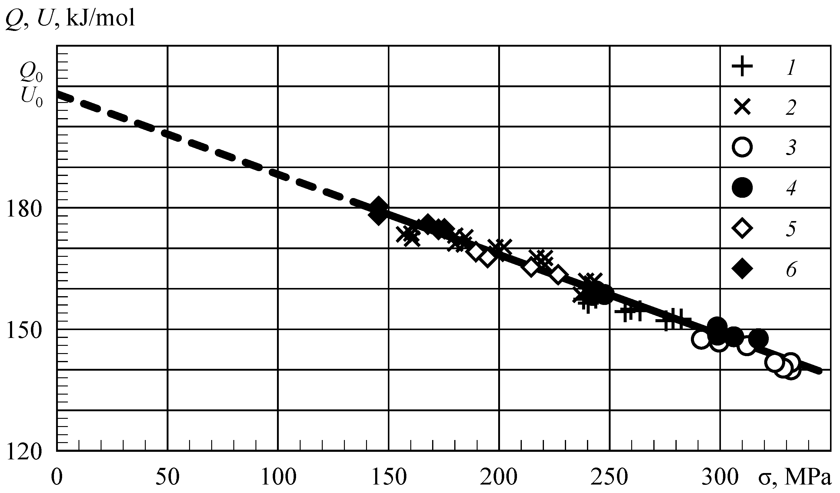
A typical relationship between deformation and fracturing is illustrated in Figure 1 [4]. And the temperature–force dependences of the steady-state creep rate are a mirror image of similar dependences of durability [2]. Using the relationship between the processes of deformation and fracturing (AED and AEF), it is possible to build mathematical models that transform external effects on the material into the kinetics of internal thermodynamic processes. As a result, the strength and deformation properties of materials observed in the experiment can be determined with calculation, reproducing the processes that determine them in models. Deviations of U(σ) and Q(σ) from straight lines indicate changes in the structure of the material and require appropriate modeling [1,5].
3. Mathematical Modeling of the Rheological Properties of the Material
New models describing their plastic flow have been introduced into the rheology of materials [6]. In material models, instead of the viscous flow bodies N (Newton body), the plastic flow bodies Zh (Zhurkov body) and Km (Kauzmann body) are used, named after these famous scientists who made a fundamentally important contribution to the study of the kinetics of thermally activated processes [7,8].
Expressing the rate of plastic strain (2) at a constant temperature in the form for the Zh body or for the Km body, where and , with in-series connection of these bodies with the Hooke solid having an elastic modulus M, we obtain the differential equations of their deformation [6]:
Or
For a constant deformation rate , we obtain the solution, for example, of Equation (3) in the form:
For a constant loading rate , the solution of Equation (3), which is the dependence of strain on time, takes the form:
where and are the stress and strain at the time , respectively.
At , Equation (5) yields the flow stress (yield stress):
This depends on the strain rate and temperature. By fixing the material strain reached, one can calculate the stress relaxation with the following formula [6]:
The relaxation process occurs without the work of external forces, i.e., due to the internal energy of a solid body, the measure of which is the temperature [3].
The parallel connection of the Hooke body with the Zh or Km body leads to solutions describing local plastic strains associated with fatigue failure. This process also occurs in time, and the composition of the structural elements of the material model makes it possible to reproduce any arbitrary type of temperature–force loading using time steps, representing the implementation of this process as a piecewise linear dependence [1]. The result of the calculations will be the values of conditional damage distributed over local volumes of material, each of which is represented by a structural element of the model. The durability of the entire structure will determine the local volume, the rate of damage accumulation in which it has maximum value. And this, in turn, will depend on the temperature, the character of stress changes, and the time spent under load.
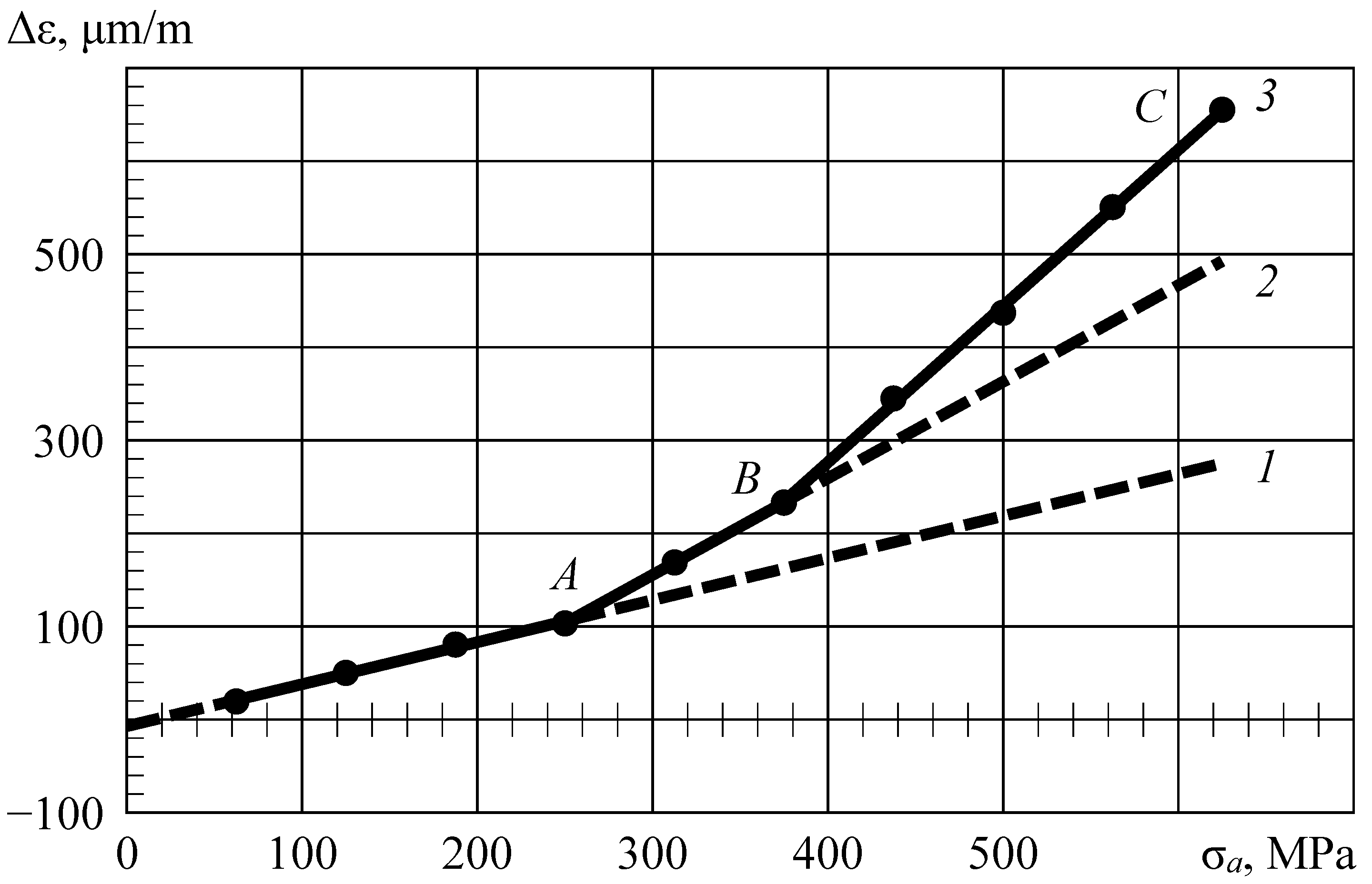
Parametric identification of the structural model of the material is performed based on the amplitude dependence of the inelasticity by dividing it into components that characterize each structural element. The typical amplitude dependence of the inelastic deformation of the material in the form of the opening of the inelasticity loop is shown in Figure 2. The same dependence can be constructed for Man-Ten steel according to Table C-4 from the publication [9].
The broken line 3 in the figure shows the value of the loop width: the maximum distance between the loading and unloading curve ε = f(σ), calculated at a constant mean value of the cycle stresses. The data are taken from an experiment performed on unidirectional carbon fiber-reinforced plastic [11]. Up to point A (line 1), there is always relaxation-type inelasticity in any material [12]. As the loading amplitude increases, hysteresis-type inelasticity additionally appears (segment AB on line 2). This is followed by a new increase in inelasticity (segment BC). Each loop width increment is ascribed to one structural element of the material model, which will determine its durability in the corresponding range of amplitudes.
The dependence of durability on mean cyclic stresses is taken into account in the rheological model of the material by changing the loop width through the change of the parameter in Equation (2). For this purpose, in each amplitude range, it is necessary to test with a different asymmetry index [1], and the endurance value N (the number of cycles passed during the specimen fracture) will be inversely proportional to the increment of the loop width in this range.
After parametric identification of the mathematical model carried out using experimental data for a specific frequency and temperature of tests, it is possible to proceed to calculations of the durability of the material under arbitrary changes in temperature and stress within the studied range of temperature–force dependences of AED and AEF. When the material structure changes, the parameters A and B in Equations (3) or (4) should be replaced by functions describing the accompanying thermally activated processes or the results of some other external effects leading to these changes.
The parameters A and B of the model are determined with a thermal activation analysis of durability data from creep experiments of material specimens (Figure 1) according to Equation (2), and the modulus of elasticity M is equal to the modulus of elasticity of the material at a given test temperature.
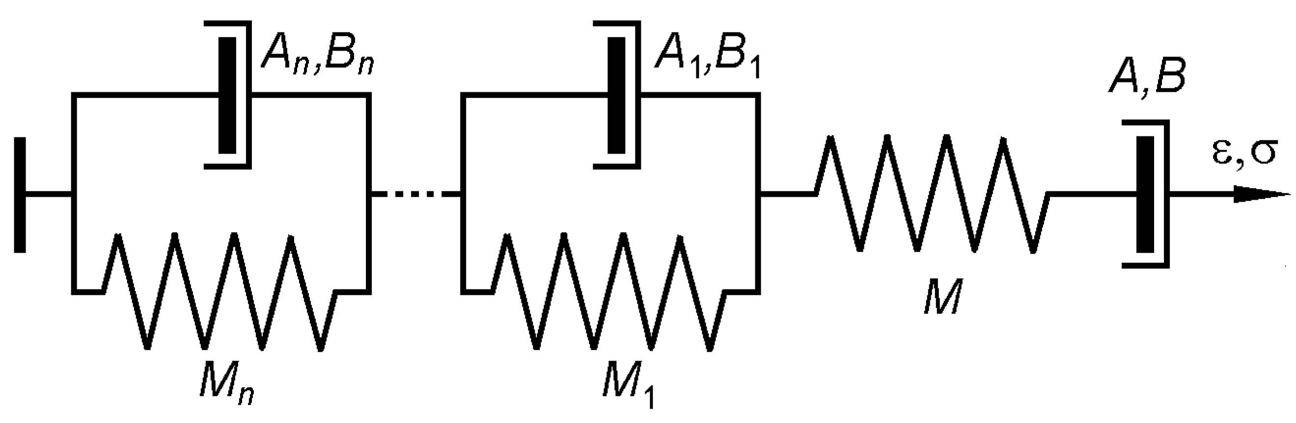
Figure 3 shows a one-dimensional structural model of the material, describing both its general flow (creep) and local plastic strains distributed over the volume of the material, varying over time and associated with fatigue failure. Having the realization of temperature–force loading conditions, it is possible to calculate any arbitrary process using time steps. Similar models with the Saint-Venant body are known and acceptable for special cases, but they are not filled with physical content and cannot reproduce temperature–time effects [13].
When testing full-scale structures, the model permits estimating errors of the bench test programs, which usually exclude the high-frequency components of the spectrum of its real loading in operation. Although the dispersion of the process at high loading frequencies is small, it makes a significant contribution to the fracturing and reduces the durability [1]. To do this, it is necessary to calculate the durability in dangerous places of the structure using time steps according to the bench test program and according to the real realizations of the loading of the same places in operation. If the durability of a certain place in the structure under loading in operation and in tests is determined with the same structural element of the material model, then the equivalent is correctly characterized by the ratio of the fracture times. Otherwise, with a forced loading program, it is necessary to calculate it using the damage accumulated with the element of the model that determines the durability of the structure in operation.
The fact that damage appears in different places in the structure of the material can be observed with a microscope [14]. This is also evidenced by indirect data obtained in the following experiment.
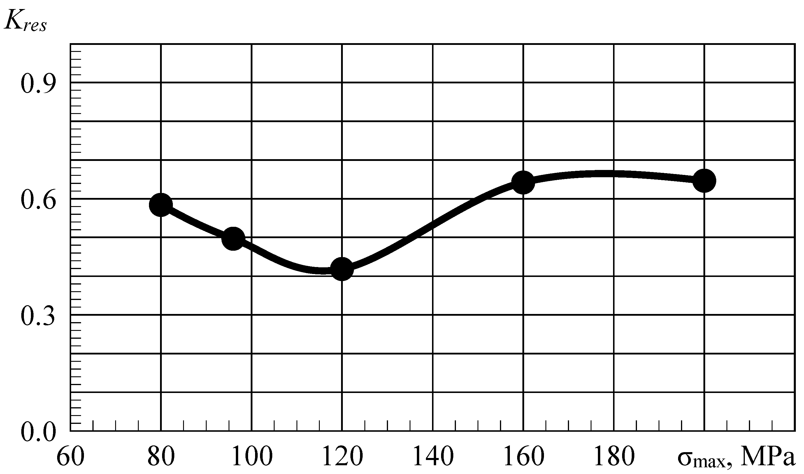
Fatigue tests were carried out on specimens cut from an aircraft wing panel after 25,000 h of operation. The specimens had countersunk holes that were loaded in operation. On specimens of another batch, cut from the same panel, where the stress level was low, and there were no cutouts, the same holes were made that did not work in operation. The ratios of the average logarithmic values of the endurance of specimens of both batches with damaged (Nd) and undamaged (N0) holes are shown in Figure 4. The panel material belongs to the Al-Cu-Zn system.
The tests were carried out with a constant value of the asymmetry index a = σm/σa = 1.222 (σmin/σmax = 0.1) at a frequency of 2.5 and 5 Hz. That is, the tests were conducted for cyclic tension with a slight excess of the mean nominal cycle stresses σm over the amplitude σa. Since the inelastic strain according to Equation (7) decreases in proportion to the increase in the logarithm of the frequency (or the rate of deformation—the stress in the local volume of the material increases), the endurance will not differ significantly, and all the results can be presented in a single dependence N(σmax).
Figure 4 shows that under loading at σ = 66 ± 54 MPa, the endurance ratio has a minimum. This means that this mode is close to the loading conditions in operation. In this mode, the damage accrued in the material in operation continues to develop “in the best way”. In other loading modes, the residual endurance shows an incorrect result. The obtained minimum of Kres ≈ 0.4 shows that, judging by this place of structure, the aircraft can be operated for about 16,000 more hours, of course, with the control of the state of the structure.
Therefore, damage according to the mathematical model of the material is calculated independently from its structural elements. And the influence of damages of various origins on the total resource of the material requires special study.
The conditional damage ω, calculated for each structural element of the model, varies from 0 to 1 and is determined as an integral of the fracture rate over time:
Equation (9) satisfies the Bailey criterion [15]. This condition implies that the threshold concentration of damage is reached in some volume of the solid body. The rate of fracture is understood to be the inverse of durability:
This is for bodies with the Zh elements or
for bodies with the Km elements, if the loading conditions and material structure are constant. Equations (1) and (10) corresponding to numerous experimental data are also confirmed with a numerical experiment performed using the molecular dynamics method [16].
According to Kauzmann, Equation (4), as well as (11), take into account reverse flow through the potential barrier. They do so with the same probability in both forward and reverse directions. He was the first to apply the theory of reaction rates to the flow of solids [8]. In reality, these probabilities may differ, and some very small value of safe stresses is found in experiments [3]. Damages do appear and accumulate, but their concentration is insufficient for macro-fracturing of the solid.
The operation of the concentration criterion of fracturing is illustrated using the pictures taken with an atomic-force microscope during glass failure [17]. When the sizes of pores become comparable with the distance between them, their coalescence occurs, followed by the formation of significant discontinuity in the material that leads to crack propagation.
4. Experiments, Calculations, and Discussion of the Results Obtained
It is human nature to divide complex problems into component parts, each of which should be studied very deeply, and the problem should not be considered in its integrity, completeness, and adequacy. There are dozens of theories of creep, plasticity, and fatigue in the mechanics of deformable solids. At the same time, the physical principles of fracturing and deformation are the same. We have seen how one can obtain the two theories of plasticity (5) and (6) from one differential creep, Equation (3), if we construct these solutions in the same coordinates σ(ε) [5]. Or to obtain many “theories of plasticity” if the material has a variety of parameters representing its structure in the model (Figure 3), which can be interpreted as the variable value of B in Equation (5).
Studies have targeted an interdisciplinary approach to the problem of the destruction of solids, for example, [18]. They consider in detail various aspects of the processes, depending on certain loading conditions, the materials used and their structures, and the mechanisms of the processes. Formulas of Equations (1) and (2) are found in the chapters Yielding, Plastic flow, Fracture, Fatigue, Creep, and high temperature mechanical behaviour. A number of areas of knowledge related to the fracturing of materials are considered and explain what happens in this case. This is the knowledge necessary to understand the essence of the events taking place. Our approach does not consider the numerous details of the phenomena observed during fracturing. This is like a cross-section of the whole problem in a certain plane. It is based on the Fundamentals of the thermodynamic [18], and all types of fracturing are considered from the same positions. The formulas given above are used specifically for calculations.
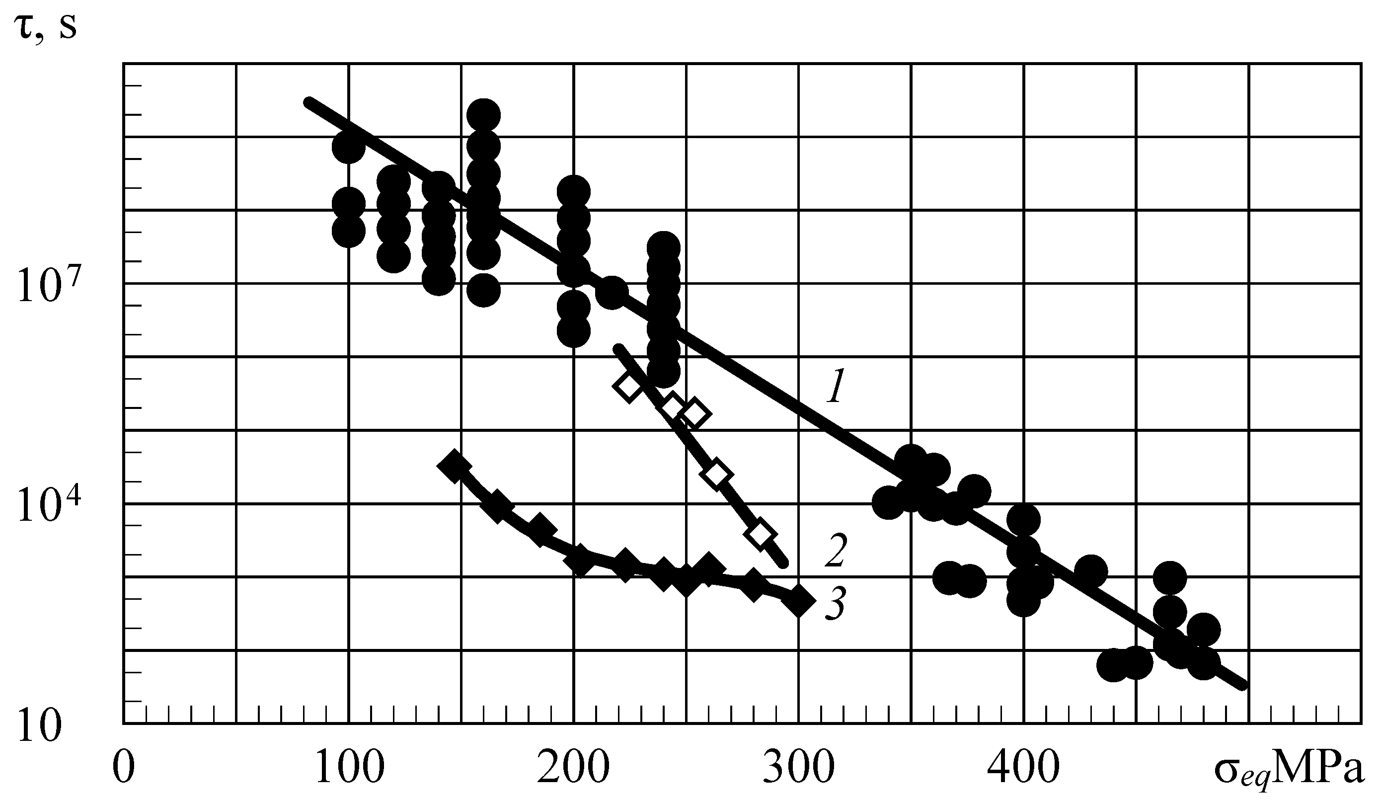
To distinguish, for example, creep from fatigue, the units of measurement of durability must be uniform. Any unit of measurement always has a physical justification and a reference value [19]. The unit of measurement “cycle” does not exist in any system of units of measurement and cannot exist, since in each case it has a different content. Therefore, it is possible to distinguish cyclic creep from fatigue only if the durability is expressed in units of time, that is, the way the failure process actually occurs. Figure 5 shows the dependences of durability on tensile stresses at their constant value and at cyclic tension with different frequencies and constant σmin = 40 MPa. The abscissa shows the equivalent stresses corresponding to the constants at which the durability has the same value in accordance with Equation (9). In this case
Figure 5 shows that at constant stresses, the logarithm of the durability linearly depends on the stresses, thereby illustrating the main regularity of fracturing (line 1). With alternating stresses varying with a low frequency (straight line 2), a decrease in the stress swing brings the value of the cyclic durability closer to the static one. It is clear that we are dealing with cyclic creep here, in which a decrease in durability occurs as a result of a concomitant relaxation of internal stresses, which decrease with a decrease in the loading rate [1,2]. If the frequency is high (curve 3), a decrease in the stress swing increases the discrepancy between the fatigue durability under static and cyclic loading, which first increases and then becomes smaller, approaching the static durability at σa → 0. With an increase in the stress swing, fatigue failure will be replaced by fracturing from cyclic creep, and curve 3 intersects with straight line 2.
If the use of Equation (12) is quite justified for a frequency of 0.05 Hz, then for fatigue failure at a frequency of 30 Hz, the approximating curve should be considered conditional (the lines in both cases are drawn according to the average logarithmic values of the durability). The process of failure during fatigue occurs in local volumes, the stresses in which are not known. In polymers, they can be evaluated with indirect methods, for example, using infrared spectroscopy [20]. In metal alloys and composite materials–structures, this can be performed with inelasticity using mathematical models based on thermodynamic laws of fracturing.
So, if it is necessary to determine the strength characteristics of a new material for using them in any calculations, the sequence of actions should be as follows. Usually, it starts with tests under monotonic loading. It is necessary to conduct a series of tests with different loading or deformation rates at several temperature values and conduct a thermal activation analysis of the test results. Since the stresses are variable, the results of processing the experimental data must be reduced, for example, to the maximum stresses recorded in each experiment. Instead of calculating the equivalent stresses σeq using Equation (12), we calculate the equivalent fracture time τeq.
The absolute value of σmax in this expression suggests that similar tests can be carried out in compression, for example, for composite materials that fracture like metals in tension, but at different levels of internal stresses [1]. In formulas of Equation (2), the sign of the strain rate should be changed accordingly to the opposite.
Then, the values are calculated, and the value of U0 is determined with the method of successive approximations. According to the type of the obtained dependences, it can be judged whether the material structure is stable in the investigated range of loading conditions. If not all U(σ) values satisfy the straight-line equation, re-processing is performed to exclude the drop-out results. According to the re-found value of U0, the dropped data is re-processed, indicating the structural changes in the material that occur in each such case. To find out the causes of deviations is the subsequent task of researchers. An example of such processing is given in the article [1], where the data are presented in Figure 5 (line 1). At the same time, the deformation characteristics of the material are estimated from the residual strain.
Having the activation parameters U0 and γ (which correspond to parameters A and B in Figure 3, respectively), it is possible to perform calculations for those loading conditions when the material flows throughout the entire volume, regardless of how the stresses and temperature change. The internal stresses in the so-called “fracture centers” naturally change, and this requires special modeling. Figure 6 shows the comparison of experimental data with the calculation for different temperature–time and temperature–force loading conditions of structural specimens made of AK-1 T1 alloy, including the data in Table 1 from the publication [1]. Vertical lines correspond to the actual scatter of durability in the experiment, if more than one specimen was tested under this loading mode.
Figure 6 shows that the calculated estimates of durability fall within a two-fold range of deviations from the experimental data, which is usually observed when testing the same material of different batches. The calculations are made taking into account the decay of a supersaturated metal solid solution in a given alloy aged to the second maximum hardness (T1 state), representing the parameter in Equation (2) as the product of the residual strain with the frequency multiplier .
The determination of the remaining parameters of the structural model of the material (Figure 3) requires cyclic loading at a constant mean stress component of the cycle σm. The values of the temperature, frequency, and shape of the loading cycle must be set. Stepwise increasing the amplitude of loading, we obtain the amplitude dependence of inelasticity (Figure 2), which is used to select amplitude values for fatigue tests according to characteristic points. That is, for example, for the AB and BC ranges, two amplitude values must be selected for each. Then, these modes must be tested with two mean load components. For each amplitude range, it is sufficient to know for any one mode the inelastic strain in the loading cycle. After parametric identification of the model, it is possible to perform calculations at a different temperature, frequency, and cycle shape, and generally at arbitrary changes in them, if one assumes that no changes in the structure occur in the material. Otherwise, this requires a separate study, and the material model parameters must be replaced by functions that represent these changes.
We present a number of experimental data and give examples of calculations. First, we show how the structural model of the material reproduces the experimental data on the basis of which its parametric identification was carried out. The parameters of the model of this material that fractured under compressive loads (in a compression half-cycle) [1] were determined with tests of specimens of carbon fiber-reinforced plastic (CFRP) T800 under a symmetric loading cycle. Figure 7 and Figure 8 show the primary experimental data and their approximation based on the model calculations, the parameters of which were obtained on the basis of the amplitude dependence of the material damage per cycle.
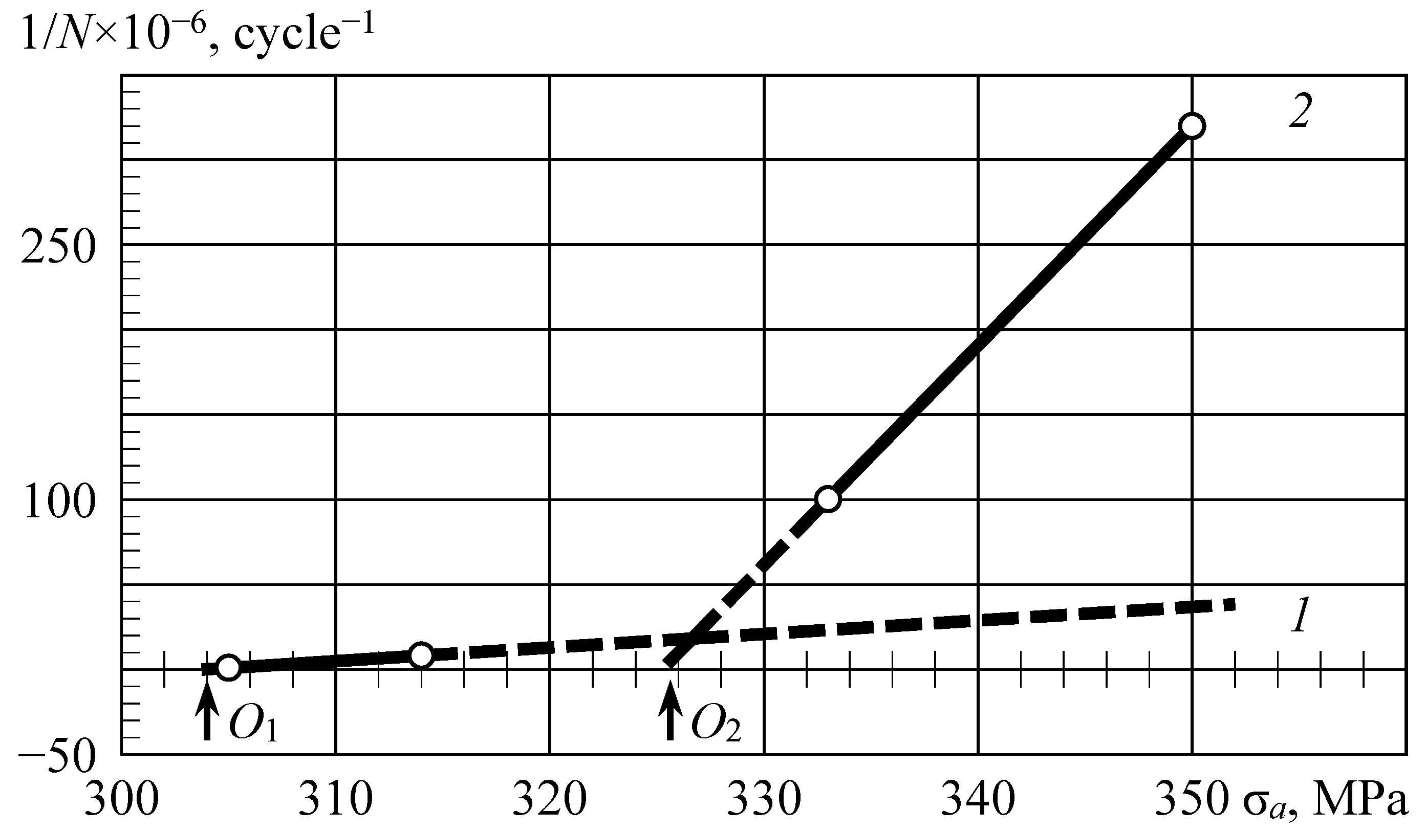
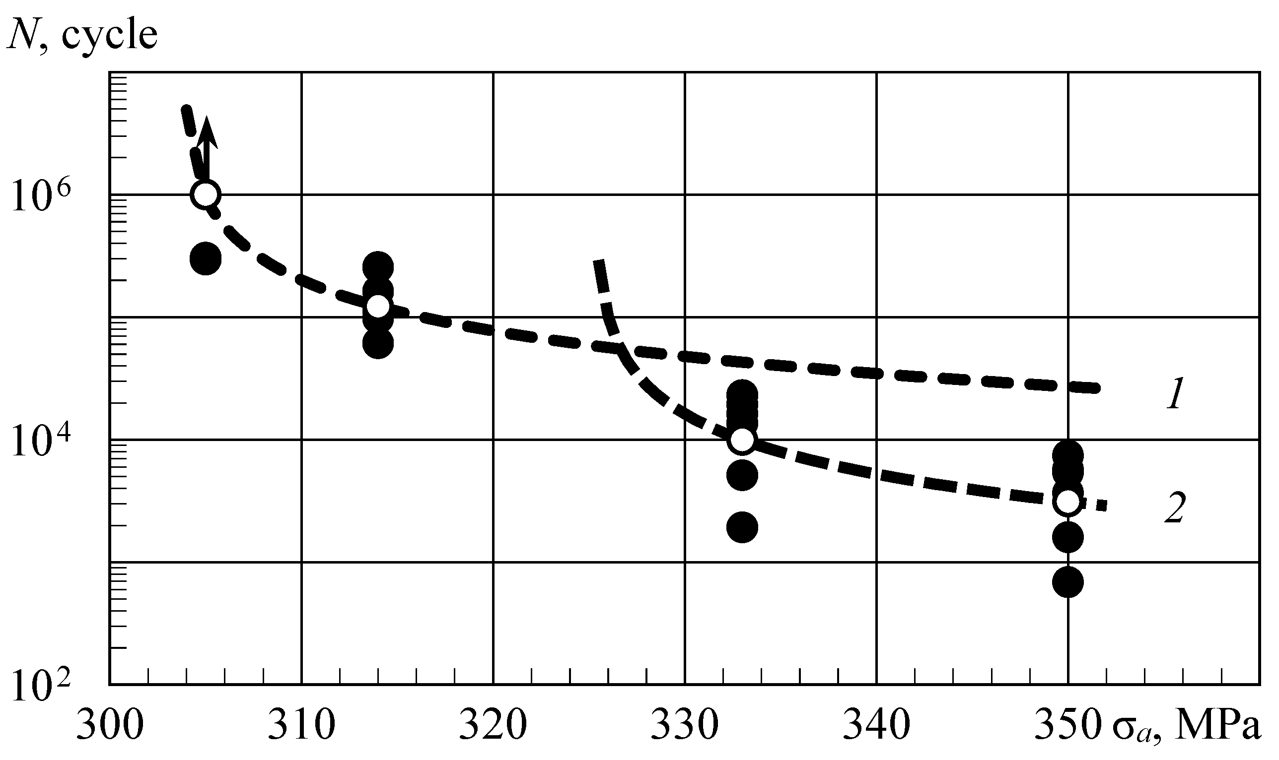
The range of loading amplitudes was from 305 to 350 MPa at test frequencies of 3 and 5 Hz, and a model with two structural elements describing plastic hysteresis in local and statistically homogeneous material volumes was constructed using four endurance values. The amplitude dependence of material damage per cycle, represented in Figure 7 by lines 1 and 2, shows that the appearance of local plastic deformations begins with an amplitude of 304 MPa (point O1), and until the point of intersection of these lines, the endurance is determined with the first structural element. Starting from the amplitude marked by point O2, local damage appears in other volumes of the material, and after the point of intersection of the lines, the endurance will be determined with the second structural element. As a result, the fatigue curve will be represented by a set of inversely proportional dependences between endurance and damage per cycle for all structural elements of the material model. For T800 CFRP, this is shown in Figure 8. In parametric identification of the mathematical model of the material, we assume for all structural elements the same value of U0, which represents the physical constant of the material for a given type of stress–strain state [2].
The dependences shown in Figure 8 for these loading conditions (cycle shape, test frequency, and temperature) in each amplitude range are formally described with expressions of the form:
where Kd is the coefficient of damage increase per cycle for lines 1 or 2 in Figure 7, σa is the loading amplitude, and σa0 is the amplitude of the appearance of plastic strains in statistically similar places of the material structure (points O1 and O2). In contrast to other versions of the formal description of fatigue curves, the parameters of Equation (14) contain quantitative characteristics of fatigue failure. The damage per cycle is equal to 1/N, calculated with the average logarithmic value of endurance for each loading mode.
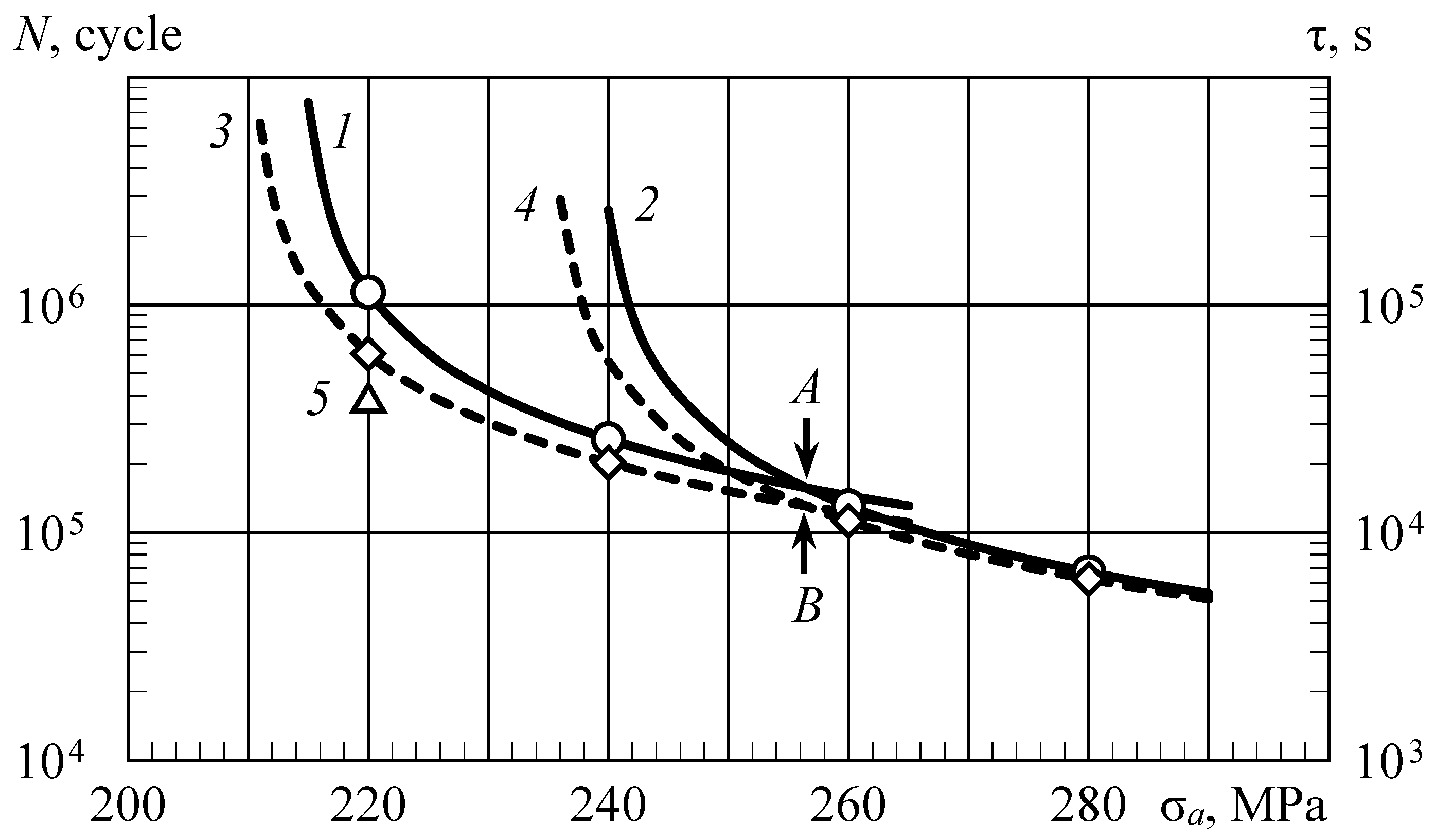
The same type of dependence was obtained for specimens made of steel 09G2S [4]. Figure 9 shows the fatigue curves as dependences of endurance or durability on the stress amplitude at two values of the mean cycle stresses. For an amplitude of 220 MPa, test data were added at σm = 90 MPa to demonstrate the linear dependence of the logarithm of endurance on the mean value of stresses in the cycle.
Tests at an amplitude of 220 MPa really show a linear relationship between the logarithm of durability (or endurance) and mean cycle stresses, which is confirmed with test data from other materials as well. Table 1 shows the values of the slope tangents of the straight lines , showing the decrease in the slope angle with an increase in the loading amplitude.
At points A and B, where curves 1, 2, 3, and 4 intersect, discontinuities or kinks in the fatigue curves can be detected if the material properties do not have too much variation and the experimental data are obtained with a small step in amplitude. V. I. Shabalin investigated this phenomenon in detail in his works [21]. Usually, ruptures are well identified when one part of specimens from the batch under given loading modes has accumulated some creep strain, and in the other part of the specimens, this has not yet occurred. This is understandable—the material structure has changed. But careful study of this phenomenon shows that there can be several discontinuities in the amplitude dependence of endurance.
If we compare the values of endurance belonging to each of these curves, with the increment of inelastic strain in the cycle, we will obtain their inversely proportional relationship. Using the example of testing specimens of CFRP (Figure 2), we will demonstrate this connection.
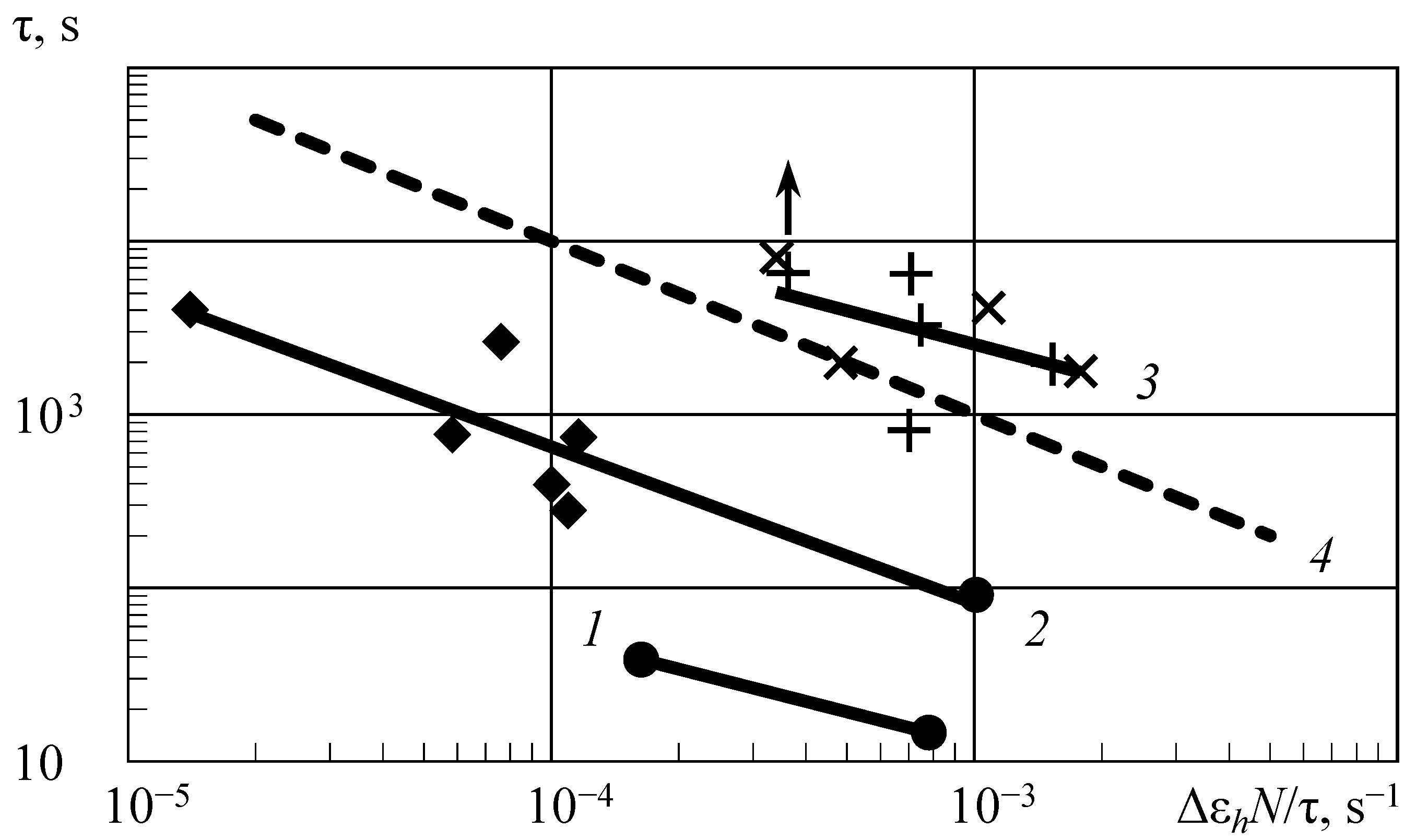
Fatigue tests were conducted on specimens of T700 CFRP with different schemes of reinforcement [11,22]. The unidirectional composite had eight layers. In two other batches of specimens, seven intermediate layers with perpendicular or diagonal stacking were added. The tests were conducted at a constant mean load component of 130 kN. Inelasticity was measured under step loading from 10 to 120 kN in steps of 10 kN. At the last step, the endurance of the specimens was determined, which was compared with the increment of inelastic strain in its last section. This corresponds to the distance between lines 2 and 3 in Figure 2. Since the specimens were tested at frequencies of 1, 2, and 3 Hz, a comparison was made between the durability and the average inelastic strain rate, similar to what is conducted in a creep analysis. The result of the comparison is shown in Figure 10 [23]. The abscissa axis plots the increment in the average inelastic strain rate as equal to the increment in the inelastic loop width due to the plastic hysteresis Δεh to the average value of the cycle period. It is equal to the ratio of durability τ to the number of cycles N passed during the failure time of the specimen.
The durability of specimens of unidirectional CFRP was distributed in two groups, which is also observed in metal alloys even in one batch of semi-finished products. Since only the longitudinally oriented layers are load-bearing (specimens are 100 mm wide with an average length of 278 mm), the specimens with an additional seven intermediate layers of another orientation had only slightly more failure time than the unidirectional ones, but they had more damping. The fundamental difference in their behavior is that the appearance of plastic hysteresis (point A in Figure 2) for specimens with orthogonal stacking occurred at a greater amplitude. The diagonal stacking of the intermediate layers apparently leads to an earlier delamination of the composite.
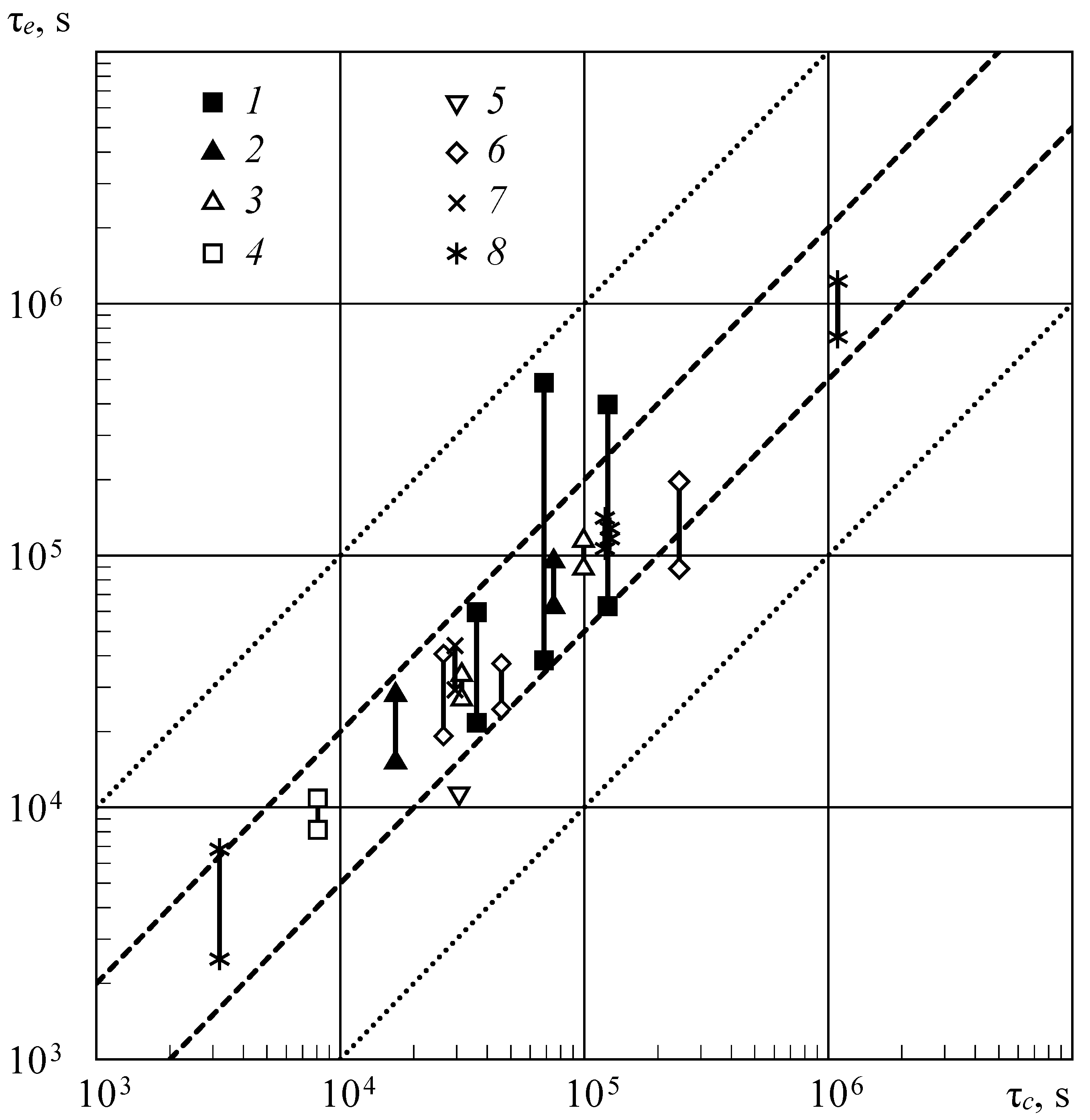
Using the relationship between inelastic strains and damage accumulation, the mathematical model makes it possible to calculate the durability for various spectra of external effects, be it stress or temperature, representing their implementation with piecewise linear approximation. Having solutions of differential Equations (3) and (4) and for other structural elements of the model at constant stresses or strains and linearly varying Equations (5) and (8), it is possible to calculate any arbitrary process of temperature–force loading [1]. Figure 11 shows a comparison of the calculated estimates of durability with experimental data for various loading cases. As in the previous example (Figure 6), the calculated estimates of durability were made using a model of a design element that transforms in time the nominal stresses or loads into strains in the places of their concentration [1,4]. The vertical lines also indicate the range of scatter in the experiment if several specimens were tested under this loading mode.
The time step of calculations for a broadband spectrum of loads is chosen to be at least 0.25–0.5 of the period of the highest frequency component of the spectrum. All load spectra were represented by equivalent polyharmonic pseudo-random processes having the same spectral density, or by a real loading process recorded in operation [24]. The degree of discreteness of the spectrum depends on the material and type of the design element.
As in the case of variable temperatures (Figure 6), the calculated estimates of durability are mainly located in the range of two-fold deviations from their experimental values. The calculations were performed based on the average statistical data of the durability of one of the semi-finished products of this material. To conduct this, two values of the mean cycle stresses are taken for each range of amplitudes, which are selected with the inelastic characteristics of the material (for example, the areas AB and BC in Figure 2).
The presented experimental data and calculation results accumulated over the last years of research work have not lost their relevance so far because they show how to approach the strength of materials in general and fatigue durability in particular. The physical principles of material fracturing and the connection of this process with plastic deformations developing over time do not depend on what kind of loading we have. This connection is embedded in mathematical models. With changes in the structure of the material, the relationship between plastic flow and failure is corrected according to experimental data.
At large absolute values of the asymmetry index and compressive loads, if the loading amplitude is insignificant or the spectral density of the process is characterized by only rare outliers, we can expect fracturing as a result of cyclic creep. In these cases, a thermal activation analysis of the obtained data should be carried out and compared with the data of monotonic loading. Thus, the T800 CFRP specimens tested with an asymmetry index of −1.947 had a very large variation in durability and were not presented in publications [1,23]. The thermal activation analysis of these data as a result of “repeated–static” loading with Formula (13) showed that the strength properties of the tested specimens fall into several strength groups. This was confirmed with software tests on flight loading implementations containing periodic emissions in the low-frequency part of the spectrum, the results of which fell into the same groups in terms of activation energy. That is, for some of the tested specimens, a large number of fluctuations of small loads did not lead to fatigue failure, and durability was determined only with residence time under load, since the maximum compression stresses were very significant.
The same result will be obtained if the test temperature is increased. Round specimens from the same material, the data on the durability of which are presented in Figure 5, were tested at a temperature of 543 K. One part of the specimens was tested at a constant stress of 200 MPa, and the other was tested with cyclic unloading of up to 20 MPa at a frequency of 10 Hz. The results of the experiment and calculation are shown in Table 2 [5].
The calculation is made based on the average statistical data of tests of specimens of this material of various batches. After the thermal activation analysis of these data and obtaining the parameters of Equation (1), calculations were performed according to Equation (9) by integrating over time steps in accordance with the shape of the loading cycle. The calculated values of durability, as we can see, fall within the range of the scatter of experimental data. And endurance, if there is a need for it, will be determined with the product of the failure time with the frequency. And when σa = σa0 according to Equation (14), when , calculations based on the structural model of the material (Figure 3) will show that the fracturing occurs as a result of cyclic creep, and the number of cycles will be determined with the failure time.
The thermofluctuation nature of fracturing also manifests itself in a complex stress state (indentation, wear, etc.), and an increasing number of researchers are using the kinetic approach to analyze the regularities of fracturing under these conditions (for example, [25,26,27]). For the rate of indentation of the indenter, an experimental dependence of Equation (2) was obtained [24]:
in which H is the pressure on the indentation area (the average value of the indentation stresses). The experimental data show a linear dependence of the logarithm of the indentation rate on H for each value of T and on the inverse value of T for each H.
When measuring hardness, we approach the “yield stress” (7) from the other side. At the initial moment, the indentation rate is high, and when the indentation area reaches a significant size, the indentation process stops. According to Equation (5), starting from low stresses, we reach it when a constant creep rate is established. Therefore, the hardness and “yield stress” are related with a linear relationship, but not leaving the origin. However, hardness and “ultimate strength” are also related with a linear relationship, but which goes from the origin [28]. The reason is that Equation (2) contains a parameter that determines the rate of plastic stain as the sum of local events, which also depends on the activation entropy [29]. The strength characteristics of the material, based on Equation (1), are associated with fracturing as a local event, which determines the difference in their relationship with hardness when maintaining comparable temperature–time conditions:
The higher the temperature and the indentation time, the lower the obtained hardness value and the corresponding “ultimate strength” σb of the material will be.
There are other works in which the phenomenon of wear is considered as a “fatigue–thermal fluctuation” process of failure (see references in the book [3]). In these works, empirical expressions were obtained—the temperature dependence of the wear rate that contains the Boltzmann factor, that is, it includes a factor of the form exp(−U/kT). The same approach is used in the work [26].
So, considering the process of fracturing as thermodynamic, it is possible, among other things, to identify structural changes in the material that have the same nature [6,10], or to analyze cases of special external effects on the material [30]. Combining knowledge and methods of mechanics, physics, and physical materials science allows us to solve such problems.
Modern approaches, for example, to fatigue failure still assume S–N curves (endurance curves) as a result [31] (and other articles on this topic previously published in the same journal). Countless such curves can be obtained. Since the dependence of endurance on the amplitude and mean stresses of the cycle are fundamentally different, we get a number of various curves. With constant values of the minimum stresses of the cycle, one series of curves is obtained. With constant values of the maximum stresses of the cycle, a different series of curves is obtained. The same variety of curves can be obtained by setting constant mean stresses of the cycle or amplitudes. Multiplying this by the set of values of frequency and temperature, we obtain the mentioned result. The shape of the cycle also has effects. The solution of the problem is not visible.
Curves of endurance are also being used if the estimation of endurance of the structural component is necessary. In the considerable approach, the calculated model of the structural component is used, which translates the time process of loading to the time strain process at the tip of the notch [4]. With such a method, the creep strain in the area of the notch is calculated, which leads to the change of the mean stress in the region of fracturing.
Curves can be used to verify calculations. And it is better to conduct tests with a polyharmonic loading process in a wide frequency range and at variable temperatures (Figure 6 and Figure 11). This will be the proof of the acceptability of the approach used. The use of S–N curves involves schematization of the real loading process and bringing it to a system of cycles. Durability calculations should be carried out according to the implementation of loading processes in time as they occur in operation. The durability of the structure is determined with flight hours and kilometers of mileage, not cycles. Schematization distorts the actual loading of structures and leads to errors, complementing them with calculation methods.
Considering only the external side of the fracture process (experimental durability curves, formal description of deformation curves, etc.) leads to what we have at the moment: dozens of strength theories, dozens of creep theories, dozens of plasticity theories, and dozens of fatigue theories. And all the curves are the result of what happens inside the material.
5. Conclusions
The proposed methodology for predicting the durability of materials in structures shows that a unified approach and reproduction in mathematical models of the processes of their failure and deformation is thermodynamic, allowing us to solve those problems that have not yet been solved with mechanical methods. Mechanics does not study what happens in a solid under load. Mechanics only delivers strain characterization and its variation, considering only the external side of the process. Therefore, its theories are far from physical reality. Only for special cases, acceptable, and sometimes even very good, solutions are obtained.
Modeling of internal thermodynamic processes, the results of which are confirmed with calculations of durability under very diverse temperature–force loading conditions, indicates the fruitfulness of the approach used. It becomes possible to take into account, in the calculations, the features in the behavior of materials associated with the influence of low temperatures and other external effects on the structure of the material and on the course of its flow and failure processes. In other words, interdisciplinary problems known in condensed matter physics are being solved.
Funding
This research received no external funding.
Data Availability Statement
Acknowledgments
The author is deeply grateful to H. D. Gringauz and N. A. Moshkin for a number of joint works that gave a lot of new, useful information and initiated the described approach, and with whose permission their results are presented here. He is also grateful to many other colleagues who, to one degree or another, helped him in numerous and laborious experiments.
Conflicts of Interest
The author declares no conflict of interest.
References
- Petrov, M.G. Mathematical modeling of failure and deformation processes in metal alloys and composites. Amer. J. Phys. Appl. 2020, 8, 46–55. [Google Scholar] [CrossRef]
- Stepanov, V.A.; Peschanskaya, N.N.; Shpeizman, V.V.; Nikonov, G.A. Longevity of solids at complex loading. Int. J. Fract. 1975, 11, 851–867. [Google Scholar] [CrossRef]
- Petrov, V.A.; Bashkarev, A.Y.; Vettegren, V.I. Physical Foundations for Predicting the Durability of Structural Materials; Polytechnic: St.Petersburg, Russia, 1993. [Google Scholar]
- Petrov, M.G. Fundamental studies of strength physics—Methodology of longevity prediction of materials under arbitrary thermally and forced effects. Int. J. Environ. Sci. Educ. 2016, 11, 10211–10227. [Google Scholar]
- Petrov, M.G. Investigation of the longevity of materials on the basis of the kinetic concept of fracture. J. Appl. Mech. Tech. Phys. 2021, 62, 145–156. [Google Scholar] [CrossRef]
- Petrov, M.G. Rheological properties of materials from the point of view of physical kinetics. J. Appl. Mech. Tech. Phys. 1998, 39, 104–112. [Google Scholar] [CrossRef]
- Tuchkevitch, V.M. Personalia of Serafim Nikolayevich Zhurkov—The occasion of his 70th birthday. Int. J. Fract. 1975, 11, 723–726. [Google Scholar] [CrossRef]
- Kauzmann, W. Flow of solid metals from the standpoint of the chemical-rate theory. Trans. AIME 1941, 143, 57–83. [Google Scholar]
- Tucker, L.E.; Bussa, S.L. The SAE cumulative fatigue damage test program. SAE Trans. 1975, 84, 198–248. [Google Scholar]
- Petrov, M.G. An Interdisciplinary Approach to Fracture of Solids from the Standpoint of Condensed Matter Physics. Adv. Sci. Technol. Eng. Syst. J. 2022, 7, 133–142. [Google Scholar] [CrossRef]
- Stepanova, L.N.; Petrov, M.G.; Chernova, V.V.; Kozhemyakin, V.L.; Katarushkin, S.A. Investigation of the inelastic properties of carbon fiber during cyclic testing of specimens using acoustic emission and strain measurement methods. Def. Fract. Mat. 2016, 5, 37–41. (In Russian) [Google Scholar]
- Nowick, A.S.; Berry, B.S. Anelastic Relaxation in Crystalline Solids; Academic Press: New York, NY, USA; London, UK, 1972. [Google Scholar]
- Michetti, A.R. Fatigue analysis of structural components through math-model simulation. Exper. Mech. 1977, 2, 69–76. [Google Scholar] [CrossRef]
- Balandin, Y.F. Thermal Fatigue of Metals in Marine Power Engineering; Shipbuilding: Leningrad, Russia, 1967. [Google Scholar]
- Bailey, J. An attempt to correlate some tensile strength measurements on glass. Glass Ind. 1939, 20, 21–25. [Google Scholar]
- Yuschenko, V.S.; Schukin, E.D. Molecular dynamics modeling in studying mechanical properties. Phys. Chem. Mech. Mat. (FKhMM) 1981, 4, 46–59. (In Russian) [Google Scholar]
- Célarié, F.; Prades, S.; Bonamy, D.; Ferrero, L.; Bouchaud, E.; Guillot, C.; Marlière, C. Glass breaks like metal, but at the nanometer scale. Phys. Rev. Lett. 2003, 90, 075504. [Google Scholar] [CrossRef] [PubMed] [Green Version]
- Yokobori, T. An Interdisciplinary Approach to Fracture and Strength of Solids; Wolters–Noordhoff Scientific Publications Ltd.: Groningen, The Netherlands, 1968. [Google Scholar]
- Kamke, D.; Krämer, K. Physikalische Grundlagen der Maßeinheiten; B. G. Teubner: Stuttgart, Germany, 1977. [Google Scholar]
- Vettegren, V.I.; Novak, I.I.; Friedland, K.J. Overstressed interatomic bonds in stressed polymers. Int. J. Fract. 1975, 11, 789–801. [Google Scholar] [CrossRef]
- Shabalin, V.I. Investigation of Fatigue of Metals at Stresses above the Yield Point. Ph.D. Thesis, VIAM, Moscow, Russia, 1970. [Google Scholar]
- Stepanova, L.N.; Petrov, M.G.; Chernova, V.V. Acoustic-emission control of inelastic properties of carbon fiber with various reinforcement schemes under cyclic loading. Cont. Diagn. 2017, 8, 18–25. (In Russian) [Google Scholar]
- Petrov, M.G. Numerical simulation of fatigue failure of composite materials under compression. In Proceedings of the XXVI Conference on Numerical Methods for Solving Problems in the Theory of Elasticity and Plasticity (EPPS-2019), Tomsk, Russia, 24–28 June 2019; Fomin, V., Placidi, L., Eds.; EPJ Web of Conferences: Les Ulis, France, 2019; Volume 221. [Google Scholar]
- Petrov, M.G. On Test Programs of Aircraft Structures. In Proceedings of the XVI International Conference on the Methods of Aerophysical Research (ICMAR 2012), Novosibirsk, Russia, 19–25 August 2012; Available online: http://www_old.itam.nsc.ru/users/libr/eLib/confer/ICMAR/2012/ (accessed on 9 September 2021).
- Kats, M.S.; Regel, V.R.; Sanfirova, T.P.; Slutsker, A.I. Kinetic nature of the microhardness of polymers. Mech. Polym. 1973, 1, 22–28. (In Russian) [Google Scholar] [CrossRef]
- Gromakovskiy, D.G. Development of a kinetic model of surface wears during friction. Probl. Mech. Eng. Automat. 1993, 6, 28–33. (In Russian) [Google Scholar]
- Gromakovsky, D.G.; Kolerov, O.K.; Logvinov, A.N.; Tregub, V.I. Estimation of the activation energy of fracture of metals and alloys by the microhardness method. Frict. Wear 1997, 18, 254–257. (In Russian) [Google Scholar]
- Markovets, M.P. Determination of Mechanical Properties of Metals by Hardness; Mechanical Engineering: Moscow, Russia, 1979. (In Russian) [Google Scholar]
- Krausz, A.S.; Eyring, H. Deformation Kinetics; John Wiley and Sons: New York, NY, USA, 1975. [Google Scholar]
- Petrov, M.G.; Lebedev, M.P.; Startsev, O.V.; Kopyrin, M.M. Effect of Low Temperatures and Moisture on the Strength Performance of Carbon Fiber Reinforced Plastic. Dokl. Phys. Chem. 2021, 500, 85–91. [Google Scholar] [CrossRef]
- Golahmar, A.; Niordson, C.F.; Martínez-Pañeda, E. A phase field model for high-cycle fatigue: Total-life analysis. Int. J. Fatigue 2023, 170, 107558. [Google Scholar] [CrossRef]
Figure 1.
Force dependence of AEF and AED of specimens of 1201 T1 alloy (Al-Cu-Mn system) tested at constant temperatures and loads; T, K: 1—398, 2—433 (creep rate); 3—398, 4—433, 5—448, 6—473 (durability).
Figure 1.
Force dependence of AEF and AED of specimens of 1201 T1 alloy (Al-Cu-Mn system) tested at constant temperatures and loads; T, K: 1—398, 2—433 (creep rate); 3—398, 4—433, 5—448, 6—473 (durability).

Figure 2.
Typical amplitude dependence of the inelasticity loop width of the material (for example, B.C.C. metals or carbon fiber-reinforced plastic): 1–3—lines of inelasticity related to different volumes of a solid, AB, BC—areas of growth of the loop width in these volumes; reprinted from Ref. [10].

Figure 3.
Structural model of a material with sequential and parallel connection of elastic bodies (Hooke’s bodies) and plastic flow bodies (Zhurkov’s or Kauzmann’s bodies).
Figure 3.
Structural model of a material with sequential and parallel connection of elastic bodies (Hooke’s bodies) and plastic flow bodies (Zhurkov’s or Kauzmann’s bodies).

Figure 4.
Dependence of the coefficient of residual endurance Kres = Nd/N0 of the design specimens on the loading mode after its long-term operation.
Figure 4.
Dependence of the coefficient of residual endurance Kres = Nd/N0 of the design specimens on the loading mode after its long-term operation.

Figure 5.
Durability of smooth specimens of AK4-1 T1 alloy (Al-Cu-Mg system) tested at constant (1) and cyclically varying with a frequency of 0.05 (2) and 30 Hz (3) stresses (temperature: 423 K); reprinted from Ref. [10].
Figure 5.
Durability of smooth specimens of AK4-1 T1 alloy (Al-Cu-Mg system) tested at constant (1) and cyclically varying with a frequency of 0.05 (2) and 30 Hz (3) stresses (temperature: 423 K); reprinted from Ref. [10].

Figure 6.
Comparison of calculated and experimental values of the durability of structural specimens and structural elements made of AK4-1 T1 alloy tested at various loads and temperatures: 1, 2—strip with a central hole and a longitudinal stringer under thermo-cyclic loading; 3—rod: constant and variable stresses at 543 K at 10 Hz; 4—full-scale structure fracture, tested under the specified temperature−force program (with addition of crack propagation period); reprinted from Ref. [10] with deletion of the range of calculated durability values, taking into account the main experimental errors in temperature and load.

Figure 7.
Amplitude dependence of damage of T800 CFRP per cycle, plotted against the logarithmic average values of endurance at σm = 0: points O1 and O2—amplitudes of appear of hysteresis type inelasticity in the different volumes of a solid; lines 1 and 2 correspond to amplitude dependences for these volumes.

Figure 8.
Amplitude dependence of the endurance of T800 CFRP and its averaged interpretation according to the mathematical model of this material; lines 1 and 2 correspond to the same lines in Figure 7.
Figure 8.
Amplitude dependence of the endurance of T800 CFRP and its averaged interpretation according to the mathematical model of this material; lines 1 and 2 correspond to the same lines in Figure 7.

Figure 9.
Calculated dependences of endurance and durability of smooth 09G2S steel specimens on loading amplitude for fracture probability of 0.5 and frequency of 10 Hz at σm = 0 (1, 2) and 50 MPa (3, 4). Point 5 is the logarithmic average value at σm = 90 MPa; the points of intersection of the curves, marked with arrows A and B, can be places of breaks in the experimental curves.

Figure 10.
Statistics of the relationship between inelasticity and durability of T700 CFRP specimens with various reinforcement schemes at P = 130 ± 120 kN: 1, 2—an eight-layer unidirectional composite (specimens of two batches); 3—the same composite with the addition of seven intermediate layers with perpendicular and diagonal packing (the arrow shows the non-failed specimen); 4—direct inversely proportional relationship; lines 1–3 indicate the distribution of specimens by strength groups.

Figure 11.
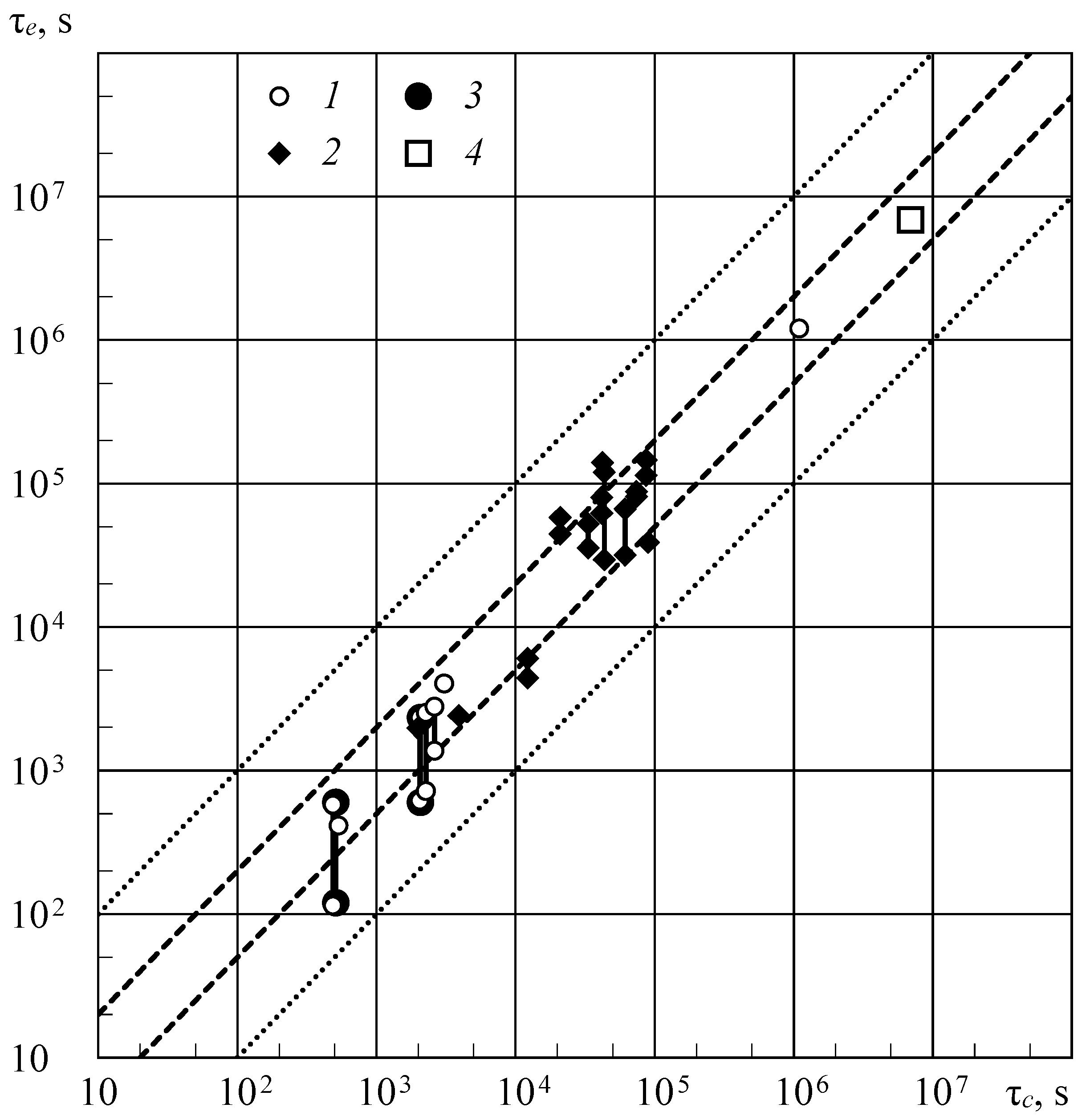
Comparison of calculated (τc) and experimental (τe) values of durability of structural specimens and structures made of 1201 T1 alloy tested under different loading programs: 1—plate–bar without notch, constant spectral density value in the interval of 0.5–10.5 Hz, 6 harmonics; 2—plate–bar without notch, narrowband random noise in the interval of 0–5.5 Hz, 13 harmonics; 3—plate–bar with notch, narrowband random noise in the interval 0–5.5 Hz, 13 harmonics; 4—plate–bar with notch, block 87-step program, triangular cycle shape at 10 Hz; 5—acoustic tests of panels in the interval of 0–200 Hz; 6—notched plate–bar, forced flight cycle of 1200 s [24], compiled from records of bending moments on the wing of an airplane–laboratory; 7—notched plate–bar, forced flight cycle GAG at 0.025 Hz; 8—30 mm wide plate–bar with a central hole of 20 mm, cyclic tests in the frequency range of 0.1–40 Hz with different cycle shape of loading; reprinted from Ref. [10] with deletion of the range of calculated durability values, taking into account the main experimental errors in load.
Figure 11.
Comparison of calculated (τc) and experimental (τe) values of durability of structural specimens and structures made of 1201 T1 alloy tested under different loading programs: 1—plate–bar without notch, constant spectral density value in the interval of 0.5–10.5 Hz, 6 harmonics; 2—plate–bar without notch, narrowband random noise in the interval of 0–5.5 Hz, 13 harmonics; 3—plate–bar with notch, narrowband random noise in the interval 0–5.5 Hz, 13 harmonics; 4—plate–bar with notch, block 87-step program, triangular cycle shape at 10 Hz; 5—acoustic tests of panels in the interval of 0–200 Hz; 6—notched plate–bar, forced flight cycle of 1200 s [24], compiled from records of bending moments on the wing of an airplane–laboratory; 7—notched plate–bar, forced flight cycle GAG at 0.025 Hz; 8—30 mm wide plate–bar with a central hole of 20 mm, cyclic tests in the frequency range of 0.1–40 Hz with different cycle shape of loading; reprinted from Ref. [10] with deletion of the range of calculated durability values, taking into account the main experimental errors in load.


Table 1.
Dependence of the slope tangent of straight lines on the amplitude of loading of 09G2S steel specimens.
Table 1.
Dependence of the slope tangent of straight lines on the amplitude of loading of 09G2S steel specimens.
| σa (MPa) | 220 | 240 | 260 | 280 |
|---|---|---|---|---|
| × 10−3 | −5.383 | −2.083 | −1.318 | −0.629 |
Table 2.
Results of tests with specimens made of the AK4-1 T1 alloy, 15 mm diameter, 60 mm length, 543 K.
Table 2.
Results of tests with specimens made of the AK4-1 T1 alloy, 15 mm diameter, 60 mm length, 543 K.
| Test Conditions | Specimen Number | Durability (s) Experiments and Calculations | |
|---|---|---|---|
| σ = 200 MPa | 1 | 120 | 510 |
| 2 | 180 | ||
| 3 | 180 | ||
| 4 | 240 | ||
| 5 | 420 | ||
| 6 | 600 | ||
| σ: 20–200 MPa Frequency: 10 Hz | 1 | 600 | 2070 |
| 2 | 2220 | ||
| 3 | 2280 | ||
| 4 | 2340 | ||
Disclaimer/Publisher’s Note: The statements, opinions and data contained in all publications are solely those of the individual author(s) and contributor(s) and not of MDPI and/or the editor(s). MDPI and/or the editor(s) disclaim responsibility for any injury to people or property resulting from any ideas, methods, instructions or products referred to in the content. |
© 2023 by the author. Licensee MDPI, Basel, Switzerland. This article is an open access article distributed under the terms and conditions of the Creative Commons Attribution (CC BY) license (https://creativecommons.org/licenses/by/4.0/).
Share and Cite
MDPI and ACS Style
Petrov, M. Fracturing of Solids as a Thermodynamic Process. Alloys 2023, 2, 122-139. https://0-doi-org.brum.beds.ac.uk/10.3390/alloys2030009
AMA Style
Petrov M. Fracturing of Solids as a Thermodynamic Process. Alloys. 2023; 2(3):122-139. https://0-doi-org.brum.beds.ac.uk/10.3390/alloys2030009
Chicago/Turabian StylePetrov, Mark. 2023. "Fracturing of Solids as a Thermodynamic Process" Alloys 2, no. 3: 122-139. https://0-doi-org.brum.beds.ac.uk/10.3390/alloys2030009