Article

Abnormal Heart Sound Classification and Model Interpretability: A Transfer Learning Approach with Deep Learning

1
School of Electrical Engineering, Computing and Mathematical Sciences (EECMS), Faculty of Science and Engineering, Curtin University, Bentley, WA 6102, Australia
2
Harry Perkins Institute of Medical Research, University of Western Australia, Crawley, WA 6009, Australia
*
Author to whom correspondence should be addressed.
J. Vasc. Dis. 2023, 2(4), 438-459; https://0-doi-org.brum.beds.ac.uk/10.3390/jvd2040034
Submission received: 26 July 2023 / Revised: 31 August 2023 / Accepted: 13 October 2023 / Published: 4 December 2023
(This article belongs to the Section Cardiovascular Diseases)

Abstract

:
Physician detection of heart sound abnormality is complicated by the inherent difficulty of detecting critical abnormalities in the presence of noise. Computer-aided heart auscultation provides a promising alternative for more accurate detection, with recent deep learning approaches exceeding expert accuracy. Although combining phonocardiogram (PCG) data with electrocardiogram (ECG) data provides more information to an abnormal heart sound classifier, the scarce presence of labelled datasets with this combination impedes training. This paper explores fine-tuning deep convolutional neural networks such as ResNet, VGG, and inceptionv3, on images of spectrograms, mel-spectrograms, and scalograms. By fine-tuning deep pre-trained models on image representations of ECG and PCG, we achieve 91.25% accuracy on the training-a dataset of the PhysioNet Computing in Cardiology Challenge 2016, compared to a previous result of 81.48%. Interpretation of the model’s learned features is also provided, with the results indicative of clinical significance.

1. Introduction

Cardiovascular disease (CVD) contributes significantly to mortality worldwide, accounting for 31% of deaths in 2019 [1]. The presence of CVD is indicated by heart sound abnormality. In order to manage CVD, prompt and accurate diagnosis must be performed. Despite this, traditional heart auscultation approaches have low accuracy rates [2,3,4]. Cardiac auscultation is a cost-effective pre-screening method that involves a physician’s interpretation of heart sounds. However, the frequencies of heart sounds are close to the boundaries of human hearing, inhibiting their accurate interpretation, thereby risking misdiagnosis [5].
Computer-aided auscultation screening presents an opportunity to detect CVD earlier than traditional approaches. Although there are many approaches to detect abnormal heart sounds, most perform poorly due to the noisy and limited datasets available. Noisy data provides challenges as classifiers rely on extracting key information to distinguish classes. Noise within the data can then hide or distort this information. Classifiers trained on limited datasets are prone to overfitting, causing poor performance on real-world data.
The complex and non-stationary nature of heart sounds makes analysis difficult. Pre-processing heart sounds can provide a cleaner input signal to the classifier. Cleaner signals lead to more accurate results. Segmenting the signal into heart sound cycles assists in detecting abnormalities such as murmurs, which are highly periodic. Segmentation is particularly important for use in clinical environments, where low signal-to-noise ratios pose a significant problem for detection. As noise from the friction of handheld stethoscopes and background sources is difficult to avoid, pre-processing methods may be used to overcome challenges to abnormal heart sound detection.
Existing state-of-the-art methods are not accurate enough for use in real-world scenarios. Recently, a start-up company, Ticking Heart, and researchers at Curtin University [6,7] worked together to create a wearable device for use in the pre-screening of CVD. The device combines up to seven phonocardiogram (PCG) signals, and one lead-I electrocardiogram (ECG) signal to provide more robust and accurate classification when compared to a single signal.
In this study, we integrate established pre-processing and segmentation techniques with transfer learning using pre-trained Convolutional Neural Network (CNN) models to enhance the performance of abnormal heart sound classification. Moreover, we delve into the interpretation of the features learned by the model. The paper is structured as follows: We begin with the ’Background’, providing context and introducing existing methodologies. Following this is the ’Materials and Methodology’ section, detailing our adopted approach. In the ’Results’ section, we present the performance of our classifier, complemented by interpretability images. Subsequent discussions about these findings are covered in the ’Discussion’ section. The paper concludes with the ’Conclusion’, summarising our key takeaways and ’Further Work’ to guide future research.

2. Background

The classification of heart sounds is commonly broken up into three main stages [8]. These stages are pre-processing, heart sound segmentation, and classification, as illustrated in Figure 1. First, a background on heart sound analysis will provide context for these stages. Then, we outline each stage, noting the established methods that have shaped our work. Lastly, the interpretable deep learning techniques utilised in our work will be explained.

2.1. Heart Auscultation

The first ( S 1 ) and second ( S 2 ) heart sounds are the most audible of the heart cycle and serve as obvious points for analysis. S 1 is caused by the closure of the atrioventricular valves at the beginning of the systole. S 2 is caused by the semilunar valves closing at the diastole’s beginning [9]. Factors such as background noise, variability in heart rhythm and pathological heart sounds complicate the detection of S 1 and S 2 [10]. Common approaches for identifying particular heart sounds include wavelet analysis and local frequency analysis [11,12,13,14].
S 1 sounds are typically found between 10 Hz–140 Hz, whereas S 2 sounds are found in the 10 Hz–200 Hz range, with most of the energy in lower frequencies of 55 Hz–75 Hz [8]. Murmur sounds are typically found in frequencies of 25 Hz to 400 Hz [10], though some have been found as high as 600 Hz [8]. With the ejection and regurgitation murmur sounds residing in higher frequencies and diseases such as mitral stenosis comprise of the lower frequencies. Filters can be designed to extract these frequency bands to perform classification.

2.2. Heart Sound Segmentation

Figure 2 shows PCG signals and the corresponding heart cycle segments. This shows an example of a healthy patient and a patient with an abnormal heart sound. The S 2 amplitude of the abnormal patient in Figure 2 was larger than the S 1 amplitude.
Schmidt et al. introduced Hidden Semi-Markov Models (HSMMs), which formed the then-state-of-the-art approach to segmentation [10]. This involved modelling the heart cycles with an HSMM, which improved on existing Hidden Markov Model approaches by allowing state duration to affect the probabilities of a state change. An extended Viterbi algorithm also allows the segmentation to start at any state. Segmentation of heart cycles allows for easier information extraction for a classifier to discern normal and abnormal heart sounds. This segmentation approach provides a base for the machine learning classifier, similar to the work by Rong et al. [6] and Potes et al. [16].

2.3. Heart Sound Classifiers

Potes et al. [16] employed an ensemble architecture consisting of a CNN combined with an AdaBoost-abstain classifier [16]. This architecture resulted in the best overall performance for the Computing in Cardiology Challenge 2016 (CinC 2016), defined as the mean of the sensitivity and specificity, both modified according to the proportion of noisy records. The architecture utilises the modified pre-processing and segmentation process described by Springer before performing heart cycle extraction and feature extraction. The extracted heart cycles are provided as input to the CNN. Furthermore, the extracted features are provided as input to the Adaboost-abstain classifier.
The CNN takes four time series inputs representing four filter bands, 25 Hz–45 Hz, 45 Hz–80 Hz, 80 Hz–200 Hz, and 200 Hz–400 Hz. A decision rule is used to combine the results of the CNN and AdaBoost-abstain classifier. If the output of either classifier is above the threshold, the PCG is classified as abnormal. It was found that the CNN by itself resulted in lower sensitivity compared to the ensemble of Adaboost and the CNN. This performance suggests there may be room for improvement of the CNN architecture or its training.
Rong et al. [6] employed an architecture similar to that of Potes et al. [16], but utilising only a CNN as the classifier and the addition of an ECG signal. This utilised the same pre-processing for the PCG signal, with the addition of an ECG signal filtered between 2 Hz–60 Hz. The four PCG bands and the single ECG band then form the five inputs into the CNN.

2.4. Convolutional Neural Networks

The introduction of large image-based CNN models has increased the accuracy of image classification tasks. The deep architecture and vast parameter space of these models allow them to identify complex patterns, local details and global contextual information. These properties enable them to extract meaningful and discriminative features from images. The performance of deep CNNs makes them suitable for abnormal heart sound detection from images such as spectrograms and scalograms.
Of the recent state-of-the-art convolutional neural networks, three that stand out include; Visual Geometry Group (VGG) [17], Residual Network (ResNet) [18], and inceptionv3 [19]. VGG stands out for its depth, ResNet for its introduction of residual blocks to the CNN architectures and inceptionv3 for its performance.

2.5. Transfer Learning

Transfer learning is a technique where knowledge learnt from a machine learning model is transferred to another model. This is usually done to reuse model knowledge learnt from one task to another. One such category of techniques utilises pre-trained neural networks as the source to be used for feature extraction or fine-tuning. Feature extraction involves taking some or all of the layers of the pre-trained network and adding some additional layers which are then trained. This serves the purpose of transferring the already learnt features to be built upon for a new task. Similarly, fine-tuning takes the pre-trained weights from the pre-trained network in addition to minimal parameters specific to the target domain, often at the final output layer. However, unlike feature extraction, the pre-trained weights are also altered during fine-tuning [20]. Utilising a pre-trained network allows data limitations to be overcome, including issues around limited labelled data for PCG and ECG datasets.
Maity et al. used fine-tuning with Yet Another Mobile Network (YAMNet) to achieve 92.23% accuracy on the entire CinC 2016 database [21]. YAMNet, a CNN model based on mobileNet, has been trained on the AudioSet-YouTube corpus dataset to predict 521 audio event classes [22]. The model was altered to predict various heart diseases, taking in mel-spectrogram images as inputs. Although the original input and heart sound database are both spectrogram representations, there are minimal shared features, making the model well-suited for transfer learning. The high accuracy of the altered model demonstrates the usefulness of transfer learning for an abnormal heart sound classifier.

2.6. Interpretable Deep Learning

The recent popularity of deep neural networks has led to increased attention given to model explainability and interpretation. The complex nature of deep neural networks (DNNs) makes it difficult to understand and interpret their decisions. Approaches to improving interpretability and explainability commonly fall into three categories; visualisation methods, model distillation, and intrinsic methods. Visualisation methods express explanation by highlighting characteristics of an input that strongly influence the output. Model distillation uses a separate white-box model that mimics the output and behaviour of the DNN. Lastly, intrinsic methods are DNNs that contain an explanation along with the output [23]. We restrict our focus to visualisation and model distillation methods.
One visualisation method to be utilised is guided-backpropagation. This approach utilisies the gradients from backpropagation to guide the most important features within an image. Guided-backpropagation only includes positive features. This is done by setting normal gradients to zero at each Rectified Linear Unit (ReLU) within the network [24].
The Gradient-weighted Class Activation Mapping (Grad-CAM) method combines gradients with activation mappings [25]. From the information found in the last convolution layer, importance values for every decision are assigned to each neuron. Applying a ReLU to the linear combination results in a coarse heatmap of the same size as the convolutional feature maps contained within the last layer, providing only positive influence features. Overlaying this heatmap on the input image provides a localisation of the features considered the most responsible for the given output prediction.
One local approximation approach, called Local Interpretable Model-Agnostic Explanations (LIME), creates a sparse linear explanation for CNNs, approximating the regions of an image that contributed most to a classification [26]. This is performed by tweaking the features observed by the CNN and examining the impact that this has on the result. This provides a per-input interpretation, indicating the most important features used for the prediction of the input image.

3. Materials and Methods

The models are trained using an EVGA Nvidia RTX 3090 sourced from Perth, Australia. 
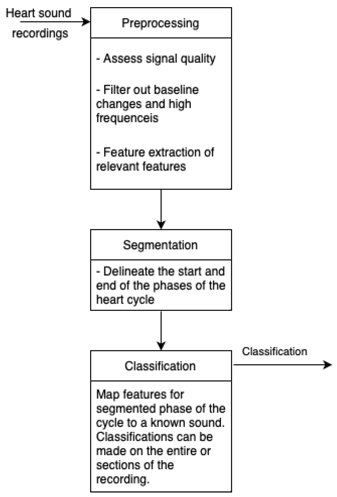
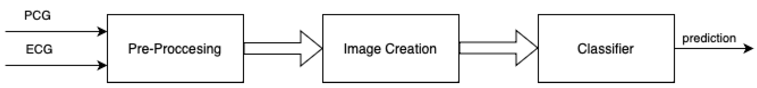
Figure 3 shows the flow of data through the system. Our methodology consisted of the following steps:
  • Pre-process the data
  • Construct an image representation
  • Train the models
  • Evaluate the models
  • Interpret the best model using explainable AI approaches
Figure 3. Classification process.
Jvd 02 00034 g003

3.1. Dataset

A subset of the CinC 2016 dataset was used for training and testing. The CinC 2016 dataset contains data from clinical and isolated environments from multiple research groups worldwide. The databases collectively offered 2435 recordings from 1297 distinct patients [8]. After breaking down longer recordings into shorter snippets and leaving out the maternal-fetal database, the competition utilised 4430 samples gathered from 1072 individuals. These samples correspond to 233,512 individual heart sounds, 116,865 cardiac cycles, and almost 30 h of PCG data.
Our work examines the classification of abnormal heart sounds by combining PCG and ECG data. As such, only the training-a database, which provides combined PCG and ECG data, is used. The training database contains 409 recordings, 4 of which do not include ECG signals, so they have been excluded. Hence, 405 different PCG recordings with an associated ECG recording are used. The dataset was split 60-20-20 train-validation-test.

3.2. Pre-Processing

Pre-processing of the data, summarised in Figure 4, is used to reduce noise and segment heart cycles. The pre-processing involved is the same as the work of Rong et al., [6] which is derived from Potes et al. [16] The PCG signal is first resampled down to 1k Hz before being bandpass filtered between 25 Hz and 400 Hz. Spikes are removed using the approach from Schmidt et al. [27]. If used, the ECG signal is resampled to 1k Hz and bandpass filtered between 2 Hz and 60 Hz. The HSMM-based approach by Springer et al. is used to segment the heart sounds, which are then used to split the data into heart cycles. The ECG data is split at the same samples as the PCG. The first 10 heart cycles of each patient are then extracted, with the 10 fragments used as separate inputs to train the model. For the approaches where the PCG data is to be split into multiple bands, the bands used are 25 Hz–45 Hz, 45 Hz–80 Hz, 80 Hz–200 Hz and 200 Hz–400 Hz. The PCG and ECG are then zero-padded to a size of 2500 samples, and the result used to create the corresponding image representation of a spectrogram or scalogram.

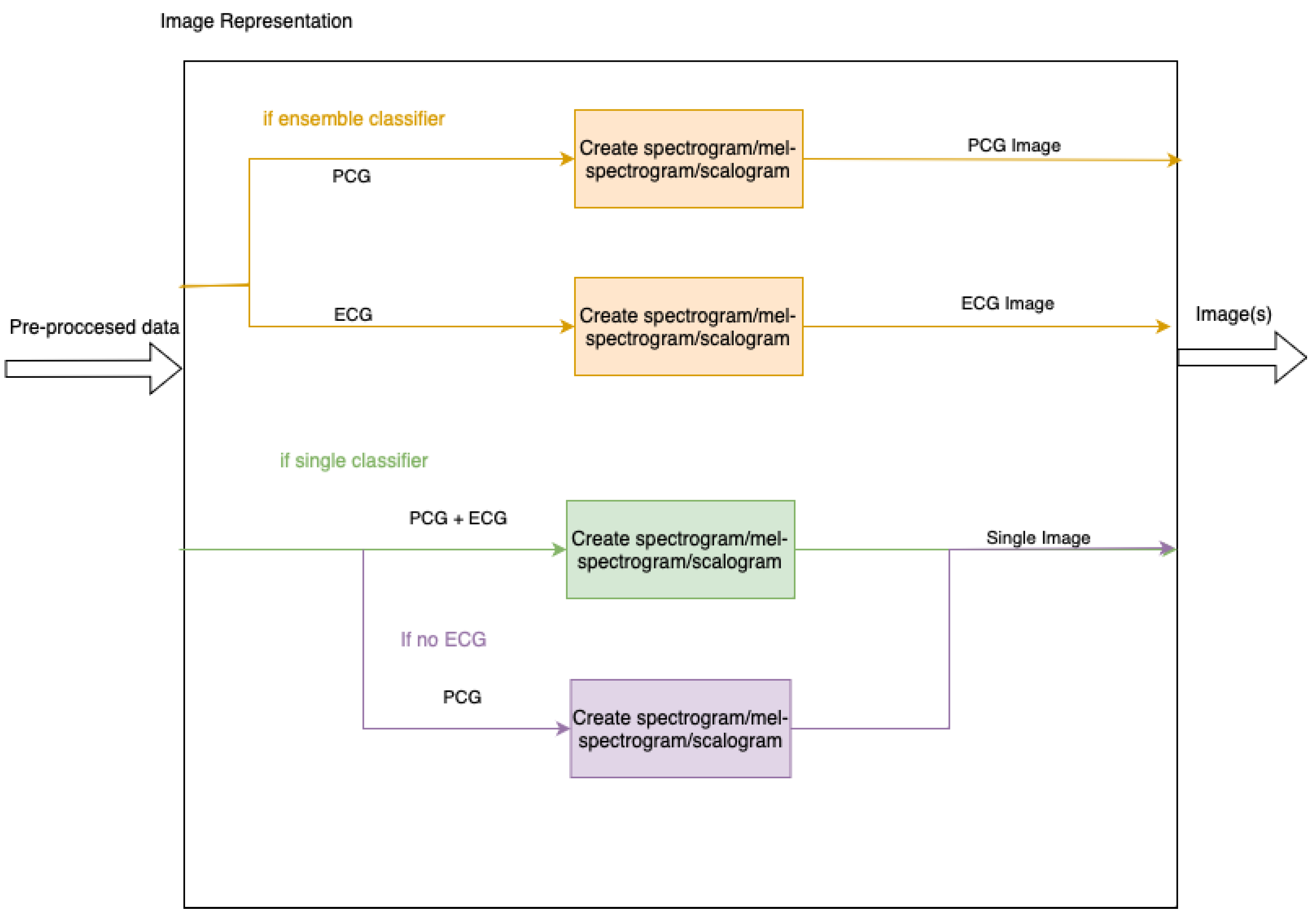
3.3. Image Representation

As each of the models uses an existing pre-trained model which takes images as input, the pre-processed data must be transformed into this format. Input images may include both PCG and ECG signals or have them as separate inputs to an ensemble of two models. The ensemble will be achieved by utilising two models, one for each image, and then adding a linear layer to combine the two. In addition to this, the PCG signal may be split into separate bands, as specified in Section 3.2. To show a clear separation between multiple bands, the images display zero-padding as white space. Figure 5 contains a high level summary of the image creation. The representations are shown below in Table 1, along with Table 2.
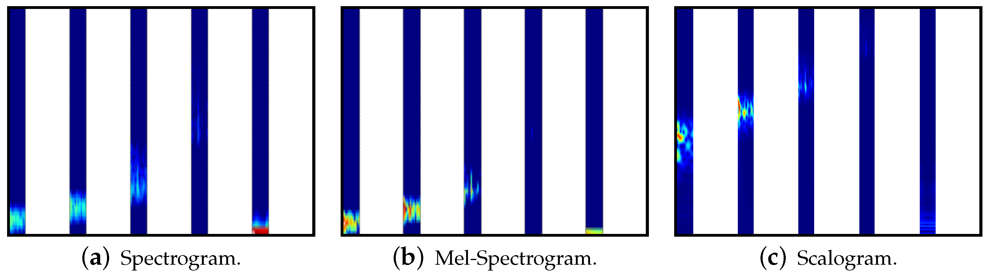
Spectrograms are created using the Short Time Fourier Transform (STFT). The STFT can be seen as taking Fourier transforms over potentially overlapping segments of the signal. This results in a two-dimensional representation of the signal showing the spectral components over time [28]. Our approach uses a window length of 100 and an overlap of 50 between each segment.
Mel-spectrograms differ from linear spectrograms in that they use the mel-scale for frequency. This more accurately models humans hearing perception. This transformation can be performed by combining the STFT with a mel filter bank, applying the transformation through the use of multiple non-uniform triangular filters [29]. Our approach uses 64 mel bins, a window length of 100 and an overlap of 50.
Scalograms show how the continuous wavelet transform (CWT) changes over time. One axis of the scalogram represents time and the other represents the reciprocal of the frequency, known as the scale [28]. By using scales instead of a fixed window length, the CWT avoids the trade-off between time resolution and frequency resolution. Although the CWT results in better time and frequency resolution than the STFT, it is more computationally complex and often results in blurry images. This can be overcome using a method called synchrosqueezing [30]. Our approach uses the synchrosqueeze CWT algorithm with a Morlet mother wavelet.

3.4. Model Training

Various pre-trained models are used as the basis of the classifier, altered to take the necessary input images and output a binary classification. This is summarised in Table 3. In addition to this, the image formats used are summarised in Figure 6.
The particular variations used for each model include ResNet34, VGG19 and inceptionv3. All of these models correspond to PyTorch models trained on the ImageNet dataset. Each model has also been modified by changing the final layer to a size of two, with one neuron representing the abnormal case and the other the normal.
Where two images are required, the CNN is duplicated to have one model per image. One CNN takes the PCG image as input and the other the ECG image. A fully-connected layer is added to combine the outputs into one classification. Figure 6 illustrates the layout of these ensemble models in orange.
All models have been trained with a stochastic gradient descent optimiser, using a learning rate of 0.001 and a momentum of 0.9. We also use cross entropy loss for each model. A learning rate scheduler with a step size of 7 and multiplicative learning rate decay factor of 0.1 is used. The ResNet models use a batch size of 64 and 4 workers. Both the VGG and inceptionv3 models use a batch size of 32 and 2 workers. The ensemble models use the same batch size as the models that comprise them.
As discussed earlier, the first 10 recording fragments for each patient are used for training. For determining a patient’s case, a decision rule is applied to all 10 fragments. As a result, there is a fragment and patient accuracy associated with each model. The fragment accuracy will be optimised during training as a higher fragment accuracy generally results in a higher patient accuracy. In addition to this, measures derived from the confusion matrix for each patient are used, with the most important being accuracy, sensitivity, and specificity [8].
Accuracy = TP + TN ( TP + TN + FP + FN )
Sensitivity = TP ( TP + FN )
Specificity = TN ( TN + FP )
Precision = TP ( TP + FP )
F 1 + = 2 × Precision × Sensitivity Precision + Sensitivity

3.5. Model Evaluation

The final classification result depends on the output of the 10 fragments for each patient. For each fragment, the model outputs two values that represent the expectation of belonging to the abnormal and normal classes. These values are then averaged separately across the abnormal and normal cases before the softmax function is applied. The resulting values, between 0 and 1, represent the expected probability that the patient belongs to either class. The patient is classified as an abnormal case if the probability is greater than a threshold value of 0.4. This value was found through experimentation on the validation set, achieving a balance between accuracy, sensitivity, and specificity. Our primary evaluation is accuracy, followed by specificity. Specificity was chosen over sensitivity due to the data imbalance against normal cases.

3.6. Model Interpretation

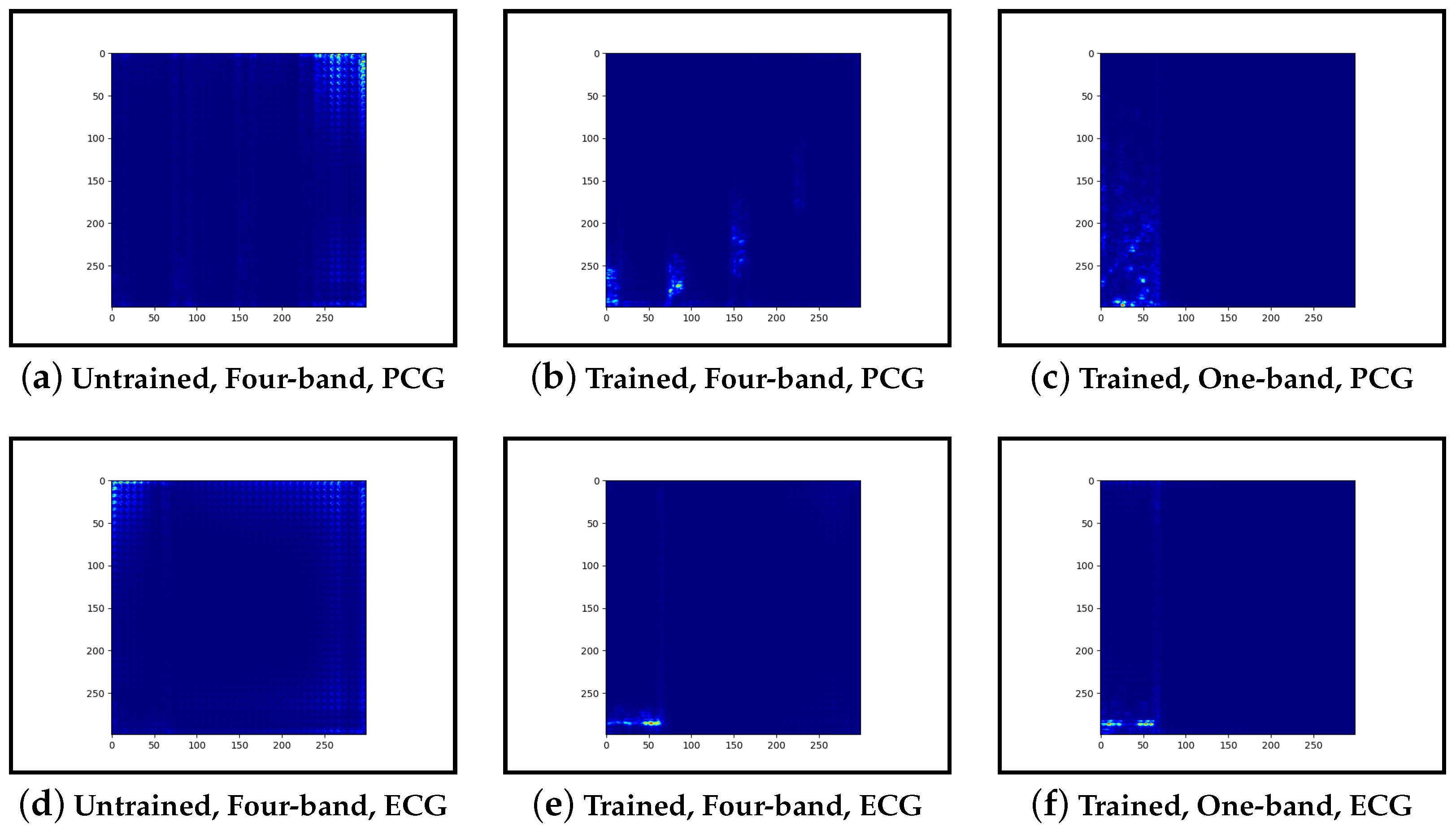
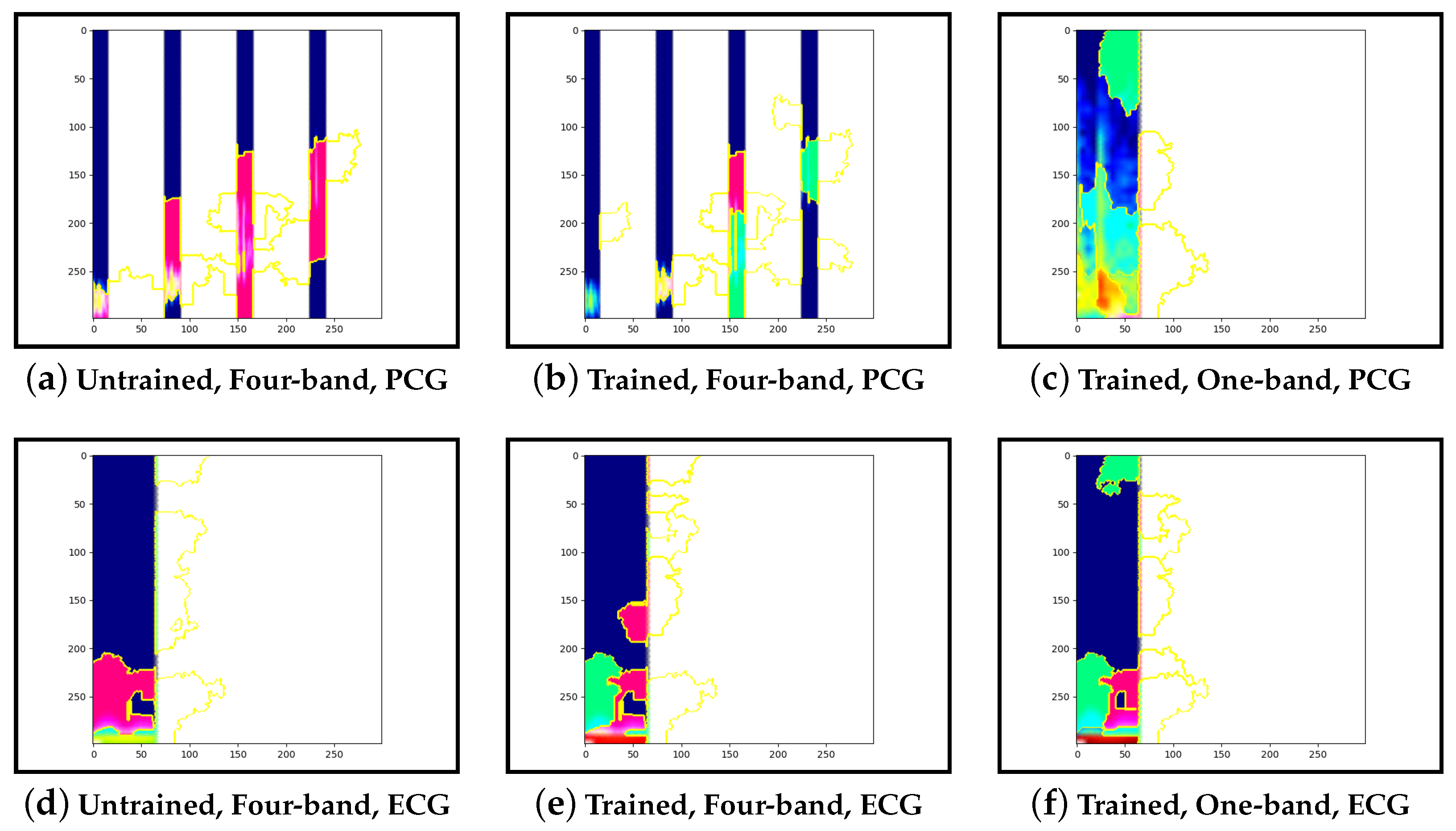
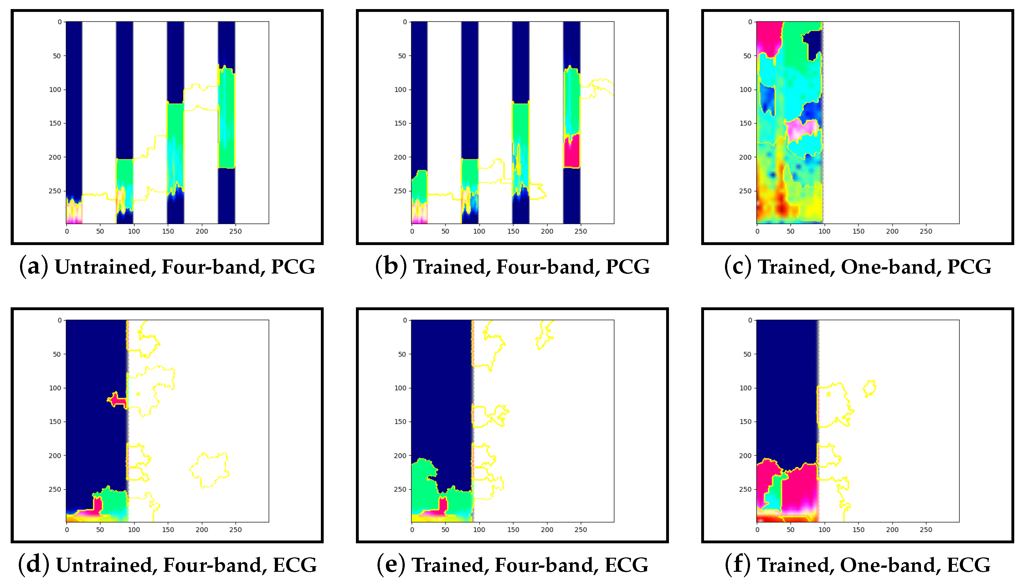
Guided-backpropagation, Grad-CAM, and LIME are used to provide interpretation of our results. Each method uses a different approach to provide a unique local interpretation. We use each method on two abnormal cases and two normal cases. These cases are taken from the test set of the model that achieved the best performance. This is then repeated for the same type of model but instead with a single band of PCG in the input image. Lastly, we compare the results against pre-trained models that are not fine-tuned. From this, we expect to see a progression from the features learnt from the ImageNet dataset to the features learnt from our training set.

4. Results

4.1. Generated Images

Figure 7 shows the generated images for each transform with the combined four-band PCG and single ECG inputs. Figure 8 shows the generated image for each transform with the separated single band PCG and single ECG inputs. These images are from the third heart cycle of entry a0009 from the CinC 2016 training-a dataset.

4.2. Classifier Model Performance

Table 4 shows the test statistics for the best performing model for each of the three input image types and the associated data type used. The best overall performing model is shown in bold. Table A1, Table A2 and Table A3 from the Appendix A show the full results of all tested models for the spectrogram, mel-spectrogram, and scalogram inputs, respectively. Interestingly, for all three images and three models, using 4 bands PCG combined with ECG achieves the best results.
Table 5 compares our best overall classifier with the classifier from Rong et al. [6], which was also trained and tested on the training-a dataset. Our model cannot be directly compared with the classifiers used in the original CinC 2016 challenge. The CinC 2016 challenge models were trained on additional databases. These databases did not include ECG signals, so these models were trained and tested only on PCG. In contrast our model is trained and tested on only one of these databases and uses both the PCG and ECG signals. From these differences a direct comparison cannot be made.

4.3. Interpretability

We provide the guided-backpropagation, Grad-CAM, and LIME images for our best performing model, inceptionv3. The guided-backpropagation method shows the areas of the image that the model used to give its classification, only including positive contributions. The Grad-CAM method combines this information with activation mappings, visualising the results as a heatmap. The LIME method shows regions that contributed positively to a correct prediction with green and negatively to a correct prediction with red, regardless of whether the prediction was normal or abnormal.
Results are provided for normal patient a0189, normal patient a0155, abnormal patient a0005 and abnormal patient a0057. Results are organised by patient and then subdivided by method. For each method, we display the untrained, four-band, and one-band results across the columns, with PCG on the top row and ECG on the bottom row. We refer to models as untrained if it is a pre-trained model without any fine-tuning.

4.3.1. Interpretability for Normal Patient a0189

Figure 9, Figure 10 and Figure 11 show the interpretability images for guided-backpropagation, Grad-CAM and LIME respectively for patient a0189. Further, each figure is broken into the PCG for an untrained model, a model with four-band PCG, a model with one-band PCG, the untrained model ECG, trained four-band model ECG, and trained one-band model ECG.

4.3.2. Interpretability for Normal Patient a0155

Figure 12, Figure 13 and Figure 14 show the interpretability images for guided-backpropagation, Grad-CAM and LIME respectively for patient a0155. Further, each figure is broken into the PCG for an untrained model, a model with four-band PCG, a model with one-band PCG, the untrained model ECG, trained four-band model ECG, and trained one-band model ECG.

4.3.3. Interpretability for Abnormal Patient a0005

Figure 15, Figure 16 and Figure 17 show the interpretability images for guided-backpropagation, Grad-CAM and LIME respectively for patient a0005. Further, each figure is broken into the PCG for an untrained model, a model with four-band PCG, a model with one-band PCG, the untrained model ECG, trained four-band model ECG, and trained one-band model ECG.

4.3.4. Interpretability for Abnormal Patient a0057

Figure 18, Figure 19 and Figure 20 show the interpretability images for guided-backpropagation, Grad-CAM and LIME respectively for patient a0057. Further, each figure is broken into the PCG for an untrained model, a model with four-band PCG, a model with one-band PCG, the untrained model ECG, trained four-band model ECG, and trained one-band model ECG.

5. Discussion

Our results show that the models that include both PCG and ECG data provided the most accurate results. The accuracy was further improved when the PCG was split into four bands. Furthermore, as shown in Table 4, with the spectrogram input data, ensemble approaches performed better than those combining the PCG and ECG data into one image. From Table A1, Table A2 and Table A3, we can see that across each configuration, providing only the PCG data led to lower accuracy than PCG and ECG, with a difference of up to 13%. In addition to this, the spectrogram representation led to greater accuracy, followed by the mel-spectrogram. This is a desirable outcome as the spectrogram is less computationally expensive than the other representations.
Despite being less computationally demanding, the ResNet and inceptionv3-based models performed better than the VGG architecture. The inceptionv3-based ensemble model had the best overall performance, achieving an accuracy of 91.25% and specificity of 70%. This was 10% greater accuracy and almost 25% greater specificity than the CNN from Rong et al. [6], shown in Table 5. This significant difference shows improvements from the utilisation of pre-trained models.
Our interpretability results suggest that an abnormal prediction favours more energy in higher frequency PCG bands. These results are expected given that this is where murmur sounds are commonly found. This can be seen through Grad-CAM, in Figure 16b and Figure 19b, where we see very high activation for an abnormal case. Through Grad-CAM in a normal case, it is shown that there is fewer high-frequency activations and more low-frequency activations, as shown in Figure 10b and Figure 13b. Our results with LIME also convey these findings, with abnormal cases having more features within the high-frequency bands, as in Figure 17b and Figure 20b. Figure 11b and Figure 14b show normal cases with more features within low-frequency bands. Lastly, guided-backpropagation generally agrees with the previous results, as shown with the abnormal case in Figure 18b and the normal cases in Figure 9b and Figure 12b. However, Figure 15b shows lower activations in the high-frequency bands than in the other abnormal case. The results generally indicate that energy in higher frequency PCG bands is associated with abnormal features, which aligns with the literature.
The ECG band was a prominent feature shown by the high activations across all interpretability methods. As mentioned, models that included ECG as input performed better than those with only PCG. These results were expected as more information was provided to the model. The particular features within the ECG band were difficult to discern and, as such, were not explored in this work.
Examining the model that contains a single PCG band and ECG within its image, abnormal cases were associated with greater high-frequency PCG activation for both LIME and Grad-CAM. Guided-backpropagation, however, shows that one of the normal predictions is mostly based on high-frequency PCG. There was a difference in performance between the single-band PCG and four-band PCG. This suggests that splitting the PCG into multiple bands may help the model learn to extract features associated with abnormal cases, such as murmurs.
Examining the inceptionv3 model with pre-trained weights, it was observed that the model does not appear to examine the relevant clinical features. With guided-backpropagation, the model behaves as an edge detector in some cases whilst not discerning any features in others. For Grad-CAM, the model is activated across the entire image instead of within the frequency bands. The LIME images do not appear to look at specific features, instead examining broad regions of the image. Comparing these results to the trained models, they have learnt clinically-significant features. Further, it suggests that these features may be responsible for achieving high accuracy.
Our work improves on Rong et al. [6], as shown by an increase in accuracy of 10%. In addition to this, we have provided local interpretation of select samples, which indicated that the learned features were clinically-significant. However, the use of deep pre-trained models introduces additional complexity as images need to be created before classification can occur. The introduction of ECG signals reduces the amount of data available compared to the CinC 2016 challenge models. By using less data for training, our model is more likely to overfit. In addition to this, using less data for testing, it is more difficult to identify overfitting. This may lead to a less robust model as compared to the works of Potes et al. [16].
Deep learning offers potential benefits for cardiology, as shown in our work. The use of deep learning, however, raises substantial ethical and operational concerns. Ensuring the diversity of training data is paramount to prevent biases, as witnessed in other deep learning applications [31]. Overfitting remains a technical concern, where algorithms might be overly tailored to specific datasets, compromising their broader applicability. Additionally, societal unease about deep-learning-driven decisions in healthcare emphasises the need for human oversight and transparent accountability.
Furthermore, ethical concerns related to patient privacy and confidentiality present a challenge for the collection of data. As a result, only limited medical datasets are available. Extensive processes are required to anonymise medical data and make it available for use in deep learning models. Despite these challenges, AI’s supportive role, aiming to enhance, not replace, human expertise, presents promising advancements in medical practice.

6. Conclusions

Our work has extended the performance of machine learning models in classifying abnormal heart sounds using PCG and ECG signals from the CinC 2016 training-a dataset. The audio is pre-processed to remove spikes and segment the data into heart cycles. After training the model on image transformations of these fragments, the results from 10 fragments are combined to predict the patient’s case.
We achieved 91.25% accuracy by fine-tuning deep image-based CNN models with spectrograms. In addition to this, it was found that using feature engineering to split the PCG into four bands and combining this with the ECG achieved the highest accuracy.
Interpretability results indicated that our models learnt clinically-significant features. These features included murmurs in high-frequency PCG bands. Moreover, splitting the data into these bands appears to significantly improve each model’s ability to learn these features.

7. Further Work

Care will need to be taken when deploying in a real-world scenario as our work was tested on a limited dataset. The model needs to be tested against a large and diverse dataset to ensure that it generalises.
Improvements to our work include additions to the architecture and training data. Data augmentation would help to address the issues of limited data and increase robustness. For the ensemble models, the PCG CNN and ECG CNN could be trained individually on additional data from separate PCG and ECG datasets. The combining layer could also be changed to a more complex multilayer perceptron network. Fine-tuning the pre-trained CNNs on general spectrograms before the generated PCG and ECG spectrograms may also provide better results.

Author Contributions

Conceptualisation, M.M.; methodology, M.M.; software, M.M.; formal analysis, M.M.; investigation, M.M.; writing—original draft preparation, M.M. and L.A.; writing—review and editing, M.M., L.A., Y.R., S.N. and G.D.; visualization, M.M.; supervision, Y.R. and S.N. All authors have read and agreed to the published version of the manuscript.

Funding

This research received no external funding.

Institutional Review Board Statement

Not applicable.

Informed Consent Statement

Not applicable.

Data Availability Statement

We used the training-a dataset, an open-source dataset from the PhysioNet/CinC Challenge 2016. The data can be found through the following link: https://archive.physionet.org/pn3/challenge/2016/ (accessed on 15 June 2023).

Acknowledgments

We would like to thank Matthew Fynn and Anton Rieutskyi for providing feedback on our draft paper.

Conflicts of Interest

The authors declare no conflict of interest.

Abbreviations

The following abbreviations are used in this manuscript:
CVDCardiovascular Disease
PCGPhonocardiogram
ECGElectrocardiogram
CNNConvolutional Neural Network
HSMMHidden Semi-Markov Model
CinCComputing in Cardiology
VGGVisual Geometry Group
YAMNetYet Another Mobile Network
ReLURectified Linear Unit
DNNDeep Neural Network
Grad-CAMGradient-weighted Class Activation Mapping
LIMELocal Interpretable Model-agnostic Explanations
STFTShort Time Fourier Transform
CWTContinuous Wavelet Transform

Appendix A. Full Model Performance

Table A1. Model performance using spectrogram.
ModelDataAccuracySensitivitySpecificityPrecisionF1
ResnetPCG (4 bands)81.25%91.67%50.00%84.62%88.00%
ResnetPCG (1 band)73.75%96.15%32.14%72.46%82.64%
ResnetPCG (4 bands) + ECG90.00%98.30%65.00%89.39%93.65%
ResnetPCG (1 band) + ECG86.25%94.23%71.43%85.96%89.91%
Resnet EnsemblePCG (4 bands) + ECG91.25%100.00%65.00%89.55%94.49%
Resnet EnsemblePCG (1 band) + ECG78.75%100.00%39.29%75.36%85.95%
VGGPCG (4 bands)82.50%91.67%55.00%85.94%88.71%
VGGPCG (1 band)78.75%100.00%39.29%75.36%85.95%
VGGPCG (4 bands) + ECG87.50%93.33%70.00%90.32%91.80%
VGGPCG (1 band) + ECG83.75%96.15%60.71%81.97%88.50%
VGG EnsemblePCG (4 bands) + ECG87.50%95.00%65.00%89.06%91.94%
VGG EnsemblePCG (1 band) + ECG82.50%100.00%50.00%78.79%88.14%
inceptionv3PCG (4 bands)81.25%91.67%50.00%84.62%88.00%
inceptionv3PCG (1 band)72.50%94.23%32.14%72.06%81.67%
inceptionv3PCG (4 bands) + ECG90.00%98.33%65.00%89.39%93.65%
inceptionv3PCG (1 band) + ECG83.75%96.15%60.71%81.97%88.50%
inceptionv3 EnsemblePCG (4 bands) + ECG91.25%98.33%70.00%90.77%94.40%
inceptionv3 EnsemblePCG (1 band) + ECG76.25%100.00%32.14%73.24%84.55%
Table A2. Model performance using mel-spectrogram.
ModelDataAccuracySensitivitySpecificityPrecisionF1
ResnetPCG (4 bands)82.50%93.33%45.00%83.82%89.06%
ResnetPCG (1 band)68.75%100.00%10.71%67.53%80.62%
ResnetPCG (4 bands) + ECG85.00%95.00%55.00%86.36%90.48%
ResnetPCG (1 band) + ECG80.00%94.23%53.57%79.03%85.96%
Resnet EnsemblePCG (4 bands) + ECG82.50%98.33%35.00%81.94%89.39%
Resnet EnsemblePCG (1 band) + ECG73.75%100.00%25.00%71.23%83.20%
VGGPCG (4 bands)80.00%93.33%40.00%82.35%87.50%
VGGPCG (1 band)68.75%100.00%35.71%73.53%80.62%
VGGPCG (4 bands) + ECG86.25%93.33%65.00%88.89%91.06%
VGGPCG (1 band) + ECG81.25%98.08%50.00%78.46%87.18%
VGG EnsemblePCG (4 bands) + ECG86.25%96.67%55.00%86.57%91.34%
VGG EnsemblePCG (1 band) + ECG73.75%100.00%25.00%71.23%83.20%
inceptionv3PCG (4 bands)82.50%95.00%45.00%83.82%89.06%
inceptionv3PCG (1 band)75.00%100.00%28.57%72.22%83.87%
inceptionv3PCG (4 bands) + ECG90.00%98.30%65.00%89.39%93.65%
inceptionv3PCG (1 band) + ECG81.25%96.15%53.57%79.37%86.96%
inceptionv3 EnsemblePCG (4 bands) + ECG85.00%100.00%40.00%83.33%90.91%
inceptionv3 EnsemblePCG (1 band) + ECG78.75%100.00%39.29%75.36%85.95%
Table A3. Model performance using scalogram.
ModelDataAccuracySensitivitySpecificityPrecisionF1
ResnetPCG (4 bands)78.75%100.00%15.00%77.92%87.59%
ResnetPCG (1 band)70.00%92.31%28.57%70.59%80.00%
ResnetPCG (4 bands) + ECG76.25%90.00%35.00%80.60%85.04%
ResnetPCG (1 band) + ECG72.50%100.00%21.43%70.27%82.54%
Resnet EnsemblePCG (4 bands) + ECG80.00%100.00%45.00%84.51%91.60%
Resnet EnsemblePCG (1 band) + ECG73.75%98.08%28.57%71.83%82.93%
VGGPCG (4 bands)77.50%100.00%10.00%76.92%86.96%
VGGPCG (1 band)71.25%98.08%21.43%69.86%81.60%
VGGPCG (4 bands) + ECG76.25%98.33%10.00%76.62%86.13%
VGGPCG (1 band) + ECG75.00%96.15%35.71%73.53%83.33%
VGG EnsemblePCG (4 bands) + ECG78.75%100.00%15.00%77.92%87.59%
VGG EnsemblePCG (1 band) + ECG71.25%98.08%21.43%69.86%81.60%
inceptionv3PCG (4 bands)81.25%98.33%30.00%80.82%88.72%
inceptionv3PCG (1 band)73.75%100.00%25.00%71.23%83.20%
inceptionv3PCG (4 bands) + ECG82.50%95.00%45.00%83.82%89.06%
inceptionv3PCG (1 band) + ECG77.50%98.08%39.29%75.00%85.00%
inceptionv3 EnsemblePCG (4 bands) + ECG81.25%100.00%25.00%80.00%88.89%
inceptionv3 EnsemblePCG (1 band) + ECG73.75%96.15%32.14%72.46%82.64%

References

  1. WHO. Cardiovascular Diseases (CVDs); WHO: Geneva, Switzerland, 2021. [Google Scholar]
  2. Chizner, M.A. Cardiac Auscultation: Rediscovering the Lost Art. Curr. Probl. Cardiol. 2008, 33, 326–408. [Google Scholar] [CrossRef] [PubMed]
  3. Feddock, C.A. The Lost Art of Clinical Skills. Am. J. Med. 2007, 120, 374–378. [Google Scholar] [CrossRef]
  4. Zhao, Q.; Niu, C.; Liu, F.; Wu, L.; Ma, X.; Huang, G. Accuracy of Cardiac Auscultation in Detection of Neonatal Congenital Heart Disease by General Paediatricians. Cardiol. Young 2019, 29, 679–683. [Google Scholar] [CrossRef]
  5. Alam, U.; Asghar, O.; Khan, S.Q.; Hayat, S.; Malik, R.A. Cardiac Auscultation: An Essential Clinical Skill in Decline. Br. J. Cardiol. 2010, 17, 8–10. [Google Scholar]
  6. Rong, Y.; Fynn, M.; Nordholm, S.; Siaw, S.; Dwivedi, G. Wearable Electro-Phonocardiography Device for Cardiovascular Disease Monitoring. In Proceedings of the 22nd IEEE Workshop on Statistical Signal Processing (SSP), Hanoi, Vietnam, 2–5 July 2023. [Google Scholar]
  7. Fynn, M.; Nordholm, S.; Rong, Y. Coherence Function and Adaptive Noise Cancellation Performance of an Acoustic Sensor System for Use in Detecting Coronary Artery Disease. Sensors 2022, 22, 6591. [Google Scholar] [CrossRef]
  8. Liu, C.; Springer, D.; Li, Q.; Moody, B.; Juan, R.A.; Chorro, F.J.; Castells, F.; Roig, J.M.; Silva, I.; Johnson, A.E.; et al. An Open Access Database for the Evaluation of Heart Sound Algorithms. Physiol. Meas. 2016, 37, 2181–2213. [Google Scholar] [CrossRef] [PubMed]
  9. Dornbush, S.; Turnquest, A.E. Physiology, Heart Sounds; StatPearls Publishing: Treasure Island, FL, USA, 2022. [Google Scholar]
  10. Schmidt, S.E.; Holst-Hansen, C.; Graff, C.; Toft, E.; Struijk, J.J. Segmentation of Heart Sound Recordings by a Duration-Dependent Hidden Markov Model. Physiol. Meas. 2010, 31, 513. [Google Scholar] [CrossRef] [PubMed]
  11. Reed, T.R.; Reed, N.E.; Fritzson, P. Heart Sound Analysis for Symptom Detection and Computer-Aided Diagnosis. Simul. Model. Pract. Theory 2004, 12, 129–146. [Google Scholar] [CrossRef]
  12. Shino, H.; Yoshida, H.; Yana, K.; Harada, K.; Sudoh, J.; Harasewa, E. Detection and classification of systolic murmur for phonocardiogram screening. In Proceedings of the 18th Annual International Conference of the IEEE Engineering in Medicine and Biology Society, Amsterdam, The Netherlands, 31 October–3 November 2002. [Google Scholar]
  13. Rajan, S.; Doraiswami, R.; Stevenson, R.; Watrous, R. Wavelet based bank of correlators approach for phonocardiogram signal classification. In Proceedings of the IEEE-SP International Symposium on Time-Frequency and Time-Scale Analysis (Cat. No.98TH8380), Pittsburgh, PA, USA, 9 October 2002. [Google Scholar]
  14. Lee, J.J.; Lee, S.M.; Kim, I.Y.; Min, H.K.; Hong, S.H. Comparison between short time Fourier and wavelet transform for feature extraction of heart sound. In Proceedings of the IEEE Region 10 Conference. TENCON 99. ’Multimedia Technology for Asia-Pacific Information Infrastructure’ (Cat. No.99CH37030), Chiang Mai, Thailand, 31 October–4 November 2003. [Google Scholar]
  15. Springer, D.B.; Tarassenko, L.; Clifford, G.D. Logistic Regression-HSMM-Based Heart Sound Segmentation. IEEE Trans. Biomed. Eng. 2016, 63, 822–832. [Google Scholar] [CrossRef] [PubMed]
  16. Potes, C.; Parvaneh, S.; Rahman, A.; Conroy, B. Ensemble of Feature-Based and Deep Learning-Based Classifiers for Detection of Abnormal Heart Sounds. In Proceedings of the 2016 Computing in Cardiology Conference (CinC), Vancouver, BC, Canada, 11–14 September 2016; pp. 621–624. [Google Scholar]
  17. Simonyan, K.; Zisserman, A. Very Deep Convolutional Networks for Large-Scale Image Recognition. In Proceedings of the International Conference on Learning Representations, San Diego, CA, USA, 7–9 May 2015. [Google Scholar]
  18. He, K.; Zhang, X.; Ren, S.; Sun, J. Deep Residual Learning for Image Recognition. In Proceedings of the 2016 IEEE Conference on Computer Vision and Pattern Recognition (CVPR), Las Vegas, NV, USA, 27–30 June 2016; pp. 770–778. [Google Scholar] [CrossRef]
  19. Szegedy, C.; Vanhoucke, V.; Ioffe, S.; Shlens, J.; Wojna, Z. Rethinking the Inception Architecture for Computer Vision. In Proceedings of the 2016 IEEE Conference on Computer Vision and Pattern Recognition (CVPR), Las Vegas, NV, USA, 27–30 June 2016; pp. 2818–2826. [Google Scholar] [CrossRef]
  20. Devlin, J.; Chang, M.W.; Lee, K.; Toutanova, K. BERT: Pre-training of Deep Bidirectional Transformers for Language Understanding. arXiv 2019, arXiv:cs.CL/1810.04805. [Google Scholar]
  21. Maity, A.; Pathak, A.; Saha, G. Transfer learning based heart valve disease classification from Phonocardiogram signal. Biomed. Signal Process. Control. 2023, 85, 104805. [Google Scholar] [CrossRef]
  22. Ellis, D.; Plakal, M. YAMNet GitHub. Available online: https://github.com/tensorflow/models/tree/master/research/audioset/yamnet (accessed on 10 July 2023).
  23. Ras, G.; Xie, N.; van Gerven, M.; Doran, D. Explainable Deep Learning: A Field Guide for the Uninitiated. arXiv 2021, arXiv:cs.LG/2004.14545. [Google Scholar] [CrossRef]
  24. Springenberg, J.T.; Dosovitskiy, A.; Brox, T.; Riedmiller, M. Striving for Simplicity: The All Convolutional Net. arXiv 2015, arXiv:cs.LG/1412.6806. [Google Scholar]
  25. Selvaraju, R.R.; Das, A.; Vedantam, R.; Cogswell, M.; Parikh, D.; Batra, D. Grad-CAM: Why did you say that? arXiv 2017, arXiv:stat.ML/1611.07450. [Google Scholar]
  26. Ribeiro, M.T.; Singh, S.; Guestrin, C. “Why Should I Trust You?”: Explaining the Predictions of Any Classifier. arXiv 2016, arXiv:cs.LG/1602.04938. [Google Scholar]
  27. Schmidt, S.E.; Holst-Hansen, C.; Hansen, J.; Toft, E.; Struijk, J.J. Acoustic Features for the Identification of Coronary Artery Disease. IEEE Trans. Biomed. Eng. 2015, 62, 2611–2619. [Google Scholar] [CrossRef]
  28. Gröchenig, K. Foundations of Time Frequency Analysis; Birkhäuser: Basel, Switzerland, 2009. [Google Scholar]
  29. Quatieri, T.F. Discrete-Time Speech Signal Processing: Principles and Practice; Prentice Hall Signal Processing Series, Prentice Hall; Pearson Education: London, UK, 2006. [Google Scholar]
  30. Thakur, G.; Brevdo, E.; Fučkar, N.S.; Wu, H.T. The Synchrosqueezing algorithm for time-varying spectral analysis: Robustness properties and new paleoclimate applications. Signal Process. 2013, 93, 1079–1094. [Google Scholar] [CrossRef]
  31. Jaltotage, B.; Ihdayhid, A.R.; Lan, N.S.; Pathan, F.; Patel, S.; Arnott, C.; Figtree, G.; Kritharides, L.; Shamsul Islam, S.M.; Chow, C.K.; et al. Artificial Intelligence in Cardiology: An Australian Perspective. Hear. Lung Circ. 2023, 32, 894–904. [Google Scholar] [CrossRef] [PubMed]
Figure 1. Main stages of heart sound classification adapted from [8].
Jvd 02 00034 g001
Figure 2. Heart Sound Segmentation [15].
Jvd 02 00034 g002
Figure 4. Pre-processing of data.
Jvd 02 00034 g004
Figure 5. Creation of image representations.
Jvd 02 00034 g005
Figure 6. Composition of classifiers.
Jvd 02 00034 g006
Figure 7. Four-band PCG and ECG combined images.
Jvd 02 00034 g007
Figure 8. Individual PCG and ECG images.
Jvd 02 00034 g008
Figure 9. Guided-Backpropagation for Normal Patient a0189.
Jvd 02 00034 g009
Figure 10. Grad-CAM for Normal Patient a0189.
Jvd 02 00034 g010
Figure 11. LIME for Normal Patient a0189.
Jvd 02 00034 g011
Figure 12. Guided-Backpropagation for Normal Patient a0155.
Jvd 02 00034 g012
Figure 13. Grad-CAM for Normal Patient a0155.
Jvd 02 00034 g013
Figure 14. LIME for Normal Patient a0155.
Jvd 02 00034 g014
Figure 15. Guided-Backpropagation for Abnormal Patient a0005.
Jvd 02 00034 g015
Figure 16. Grad-CAM for Abnormal Patient a0005.
Jvd 02 00034 g016
Figure 17. LIME for Abnormal Patient a0005.
Jvd 02 00034 g017
Figure 18. Guided-Backpropagation for Abnormal Patient a0057.
Jvd 02 00034 g018
Figure 19. Grad-CAM for Abnormal Patient a0057.
Jvd 02 00034 g019
Figure 20. LIME for Abnormal Patient a0057.
Jvd 02 00034 g020
Table 1. Image representation transforms.
TypePCG Bands
Spectrogram1
Spectrogram4
Mel-Spectrogram1
Mel-Spectrogram4
Scalogram1
Scalogram4
Table 2. Image representations combinations.
PCG BandsPCG + ECGSeparate Images
4YesYes
4YesNo
4NoN/A
1YesYes
1YesNo
1NoN/A
Table 3. Classifier summary.
Model TypePre-Trained ModelData
CNNResNetPCG + ECG
CNNinceptionv3PCG + ECG
CNNVGGPCG + ECG
CNNResNetPCG
CNNinceptionv3PCG
CNNVGGPCG
CNN-EnsembleResNetPCG + ECG
CNN-Ensembleinceptionv3PCG + ECG
CNN-EnsembleVGGPCG + ECG
Table 4. Model performance.
ImageModelDataAccuracySensitivitySpecificityPrecisionF1
SpectrogramResnet EnsemblePCG (4 bands) + ECG91.25%100.00%65.00%89.55%94.49%
SpectrogramVGG EnsemblePCG (4 bands) + ECG87.50%95.00%65.00%89.06%91.94%
Spectrograminceptionv3 EnsemblePCG (4 bands) + ECG91.25%98.33%70.00%90.77%94.40%
Mel-SpectrogramResnetPCG (4 bands) + ECG85.00%95.00%55.00%86.36%90.48%
Mel-SpectrogramVGGPCG (4 bands) + ECG86.25%93.33%65.00%88.89%91.06%
Mel-Spectrograminceptionv3PCG (4 bands) + ECG90.00%98.30%65.00%89.39%93.65%
ScalogramResnet EnsemblePCG (4 bands) + ECG80.00%100.00%45.00%84.51%91.60%
ScalogramVGG EnsemblePCG (4 bands) + ECG78.75%100.00%15.00%77.92%87.59%
Scalograminceptionv3PCG (4 bands) + ECG82.50%95.00%45.00%83.82%89.06%
Table 5. Performance comparison.
ClassifierDatasetAccuracySensitivitySpecificity
CNN
(Rong et al. [6])
training-a81.48%94.92%45.45%
inceptionv3 Ensembletraining-a91.25%98.33%70.00%
Disclaimer/Publisher’s Note: The statements, opinions and data contained in all publications are solely those of the individual author(s) and contributor(s) and not of MDPI and/or the editor(s). MDPI and/or the editor(s) disclaim responsibility for any injury to people or property resulting from any ideas, methods, instructions or products referred to in the content.

