Article

Applying the Robust Chi-Square Goodness-of-Fit Test to Multilevel Multitrait-Multimethod Models: A Monte Carlo Simulation Study on Statistical Performance

by
Minne Luise Hagel
1,2,*,
Friedemann Trutzenberg
1 and
Michael Eid
1,*
1
Department of Education and Psychology, Freie Universität Berlin, 14195 Berlin, Germany
2
Department of Psychology, Humboldt-Universität zu Berlin, 12489 Berlin, Germany
*
Authors to whom correspondence should be addressed.
Submission received: 13 February 2024 / Revised: 21 March 2024 / Accepted: 22 March 2024 / Published: 29 March 2024
(This article belongs to the Section Psychometrics and Educational Measurement)

Abstract

:
As the robust maximum likelihood χ 2 goodness-of-fit test had been found to yield inflated type-I error rates for certain two-level confirmatory factor analysis (CFA) models, a new correction for the test was implemented in Mplus version 8.7. In this simulation study, we inspected whether the corrected test statistics follow the expected χ 2 distributions when applying more complex two-level models for multitrait-multimethod data with varying sample sizes and correlations within trait factors. Investigating rejection rates and probability-probability plots, we found that the new correction markedly and sufficiently reduced previously inflated rejection rates in conditions with within-trait correlations equal to 1, 100 between-level units, and 10 or 20 within-level units. In other conditions, rejection rates were hardly affected or not sufficiently reduced by the new correction. While in most conditions, 2 within-level units did not suffice, 5 within-level units and 250 between-level units were enough to yield correct rejection rates given within-trait correlations did not exceed 0.80. Correlations above 0.80 required larger sample sizes. In planning studies with multilevel CFA models, researchers should be aware that sample size requirements for likelihood-based model fit evaluations can depend on several different factors and might consider conducting Monte Carlo simulations tailored to their specific modeling conditions.

1. Introduction

Having been cited more than 5500 times, the article originally introducing multitrait-multimethod (MTMM) analysis by Campbell and Fiske [1] ranks among the most influential articles ever published in psychology [2]. MTMM analysis supposedly constitutes the most widely used method for quantifying (discriminant and convergent) construct validity [2]. Convergent validity describes the extent to which data gathered with different methods, which are thought to capture the same trait, correlate with each other, while discriminant validity describes the extent to which the measures of different traits diverge [1]. Whenever a study includes more than one trait, e.g., neuroticism, agreeableness, and intelligence, as well as more than one method, e.g., an interview, a work sample, and a recommendation letter, it can be referred to as a multitrait-multimethod (MTMM) study [2]. Since their introduction, approaches for analyzing MTMM data have advanced to various more sophisticated confirmatory factor models (CFA-MTMM models), which allow for the separate inspection of trait, method, and additional error factors and thus for a more thorough analysis of construct validity [2,3,4]. In the following, we will illustrate MTMM models referring to raters as an example of multiple methods [5]. Whenever raters are interchangeable, it is necessary to account for the nested data structure that is present due to the underlying two-step sampling procedure [4], which can be achieved via conducting multilevel CFA (MCFA).
While many software programs can perform complex statistical analyses, Mplus is probably one of the best-equipped programs for latent variable modeling [6,7]. As Mplus provides various corrections for non-normal and non-independent data with and without missing values, it is also well-equipped to deal with common problems arising in practice when applying MCFA [7]. However, Jak et al. [8] found that the χ 2 goodness-of-fit test in Mplus version 8.5 led to inflated type-I error rates when applying it to different two-level CFA models. In reaction to their finding, Asparouhov and Muthén [9] implemented a modified correction factor for the test statistic from version 8.7 on. In a small simulation study, they demonstrated that the modified correction factor, which fixes problematic parameters to values inside the admissible space, eliminates the inflated rejection rates for the models that were affected in the simulation study conducted by Jak et al. [7,8]. Since then, to the best of our knowledge, no studies have been conducted to test the new correction factor’s performance on more complex models.
The present simulation study had two aims. (1) Evaluating whether the new correction factor implemented in Mplus version 8.7 sufficiently corrects the test statistic in conditions with varying proportions of possibly problematic parameters in three more complex two-level CFA-MTMM models and (2) identifying requirements pertaining to sample sizes on both levels as well as within-trait correlations (WTC) for the χ 2 test to work as intended when working with those models. Additionally, we explored the statistical performance of the root mean square error of approximation (RMSEA) and the comparative fit index (CFI) before and after the new correction, as both of them are based on the χ 2 test statistic [10] (pp. 22–23).
The present article is structured as follows. First, we provide necessary background information on the difference between interchangeable and structurally different methods and the models we applied in the simulation study on different χ 2 test statistics and their correction factors in Mplus and on previous simulation studies reporting the performance of χ 2 test statistics for MCFA models in Mplus. Second, we describe the Monte Carlo simulation study we conducted to examine the χ 2 test statistics’ performance for varying Mplus versions, models, and sample sizes on the between- and within-level, as well as WTC. Finally, based on the results of the simulation study, we discuss the boundaries of the χ 2 test in Mplus when working with two-level CFA-MTMM models and provide recommendations on using likelihood-based model fit statistics in applied research with MCFA-MTMM models.

1.1. Interchangeable vs. Structurally Different Raters

Working with MTMM data, it is important to distinguish between interchangeable and structurally different raters, as they differ in their sampling procedure as well as in the way they need to be modeled [4]. Please note that, in this paper, we only included nested designs in which all targets are rated by distinct, non-overlapping raters, i.e., in which a given target is never rated by the same rater as any other target.

1.1.1. Interchangeable Raters

Interchangeable raters share their role to the target and stem from the same population of possible raters with the same role [5,11]. If, for example, several teachers’ capabilities for clarity, time management, and creating a supportive learning atmosphere (multiple traits) are rated by a random sample of each teacher’s students, it could be reasonable to assume that all students have the same role (being a student) and can therefore be considered interchangeable. They do not necessarily have to agree on their teacher’s capabilities, but as the amount of time and context in which they see them is similar, these students have a similar basis of information when rating. In nested designs, interchangeable raters are the result of a two-step sampling procedure [4]. In the first step, a set of level-2 units, e.g., teachers, is randomly drawn from the population of level-2 units, and in the second step, a set of level-1 units, e.g., students, is randomly drawn for each level-2 unit, e.g., teacher. Due to the nested data structure, the appropriate CFA model for interchangeable raters is an MCFA model in which raters are modeled on the within-level and traits (of targets) are modeled on the between-level [4].
Generally, in a (two-level) MCFA model, the total covariance matrix of all observed variables Σ T is decomposed into two covariance matrices: the between-level covariance matrix Σ B and the within-level covariance matrix Σ W [12,13]:
Σ T = Σ B + Σ W
The between- and within-level covariance matrices Σ B and Σ W are decomposed into covariance matrices of the (common) factors on the between- ( Ψ B ) and within- ( Ψ W ) level as well as between- and within-level residual covariance matrices Θ B and Θ W , Λ B and Λ W being the matrices of all factor loadings on the between and within level [12,13]:
Σ B = Λ B Ψ B Λ B + Θ B   a n d   Σ W = Λ W Ψ W Λ W + Θ W
Eid et al. [4] differentiate two types of MTMM models for interchangeable raters: models with heterogenous (indicator-specific) and models with homogenous (unidimensional) trait factors. In the following, those types of models are described.
In a model with heterogenous trait factors, the observed ratings ( Y trik ) for a target t assessed by rater r via the ith indicator pertaining to trait k are decomposed into an indicator-specific mean μ ik , a value on the indicator-specific trait variable T tik multiplied by its corresponding trait factor loading λ Tik , a value on the trait-specific method variable M trk multiplied by its corresponding method factor loading λ Mik , and a value on the indicator-specific measurement error variable E trik :
Y trik = μ ik + λ Tik T tik + λ Mik M trk + E trik    
The trait variables T tik are modeled on the between-level, the rater-specific method variables M trk as well as the residual variable E trik are modeled on the within-level. T tik , M trk , and E trik are assumed to have zero means. Additionally, it is assumed that all trait variables are uncorrelated with all method variables as well as all error variables, that all method variables are uncorrelated with all error variables, and that all error variables are uncorrelated. In models with heterogenous trait factors, correlations of trait factors belonging to the same trait (WTC) are not perfect (≠1) but should be very high if the observed variables are assumed to measure the same trait. Correlations between trait factors of different traits, in contrast, should be lower to indicate discriminant validity of the traits on the between-level. All factor loadings λ Tik are set to one. As interchangeable raters are the only methods in these models and as T tik , M trk , and E trik are centered, values on the trait variables T tik represent expected deviations of individual targets’ trait values from the expected value for a given indicator μ ik across raters. The method variables M trk are unidimensional within traits (not indicator-specific) but can vary between traits, which means that with these method factors, the raters’ possible over- and underestimation pertaining to a specific target and trait is modeled while over- and underestimation pertaining to a specific indicator is not. E trik contains deviations from the indicator-specific mean μ ik that are neither explained by targets’ trait values nor by the raters’ over- or underestimation of the trait values [4]. Figure 1 depicts a model with two traits, three indicators per trait, and heterogenous trait factors.
Figure 2, on the other hand, depicts a model with homogenous (unidimensional) trait factors. In models with unidimensional trait factors, all WTC equal one, one underlying trait factor T tk is modeled for each trait, and only its first-factor loading λ Tik is set to one for identification reasons, while all other λ Tik are freely estimated [4]. If all other parts of the two models are identical, a model with unidimensional trait factors is a more restrictive version of its corresponding model with heterogenous trait factors [2,4].
In the two MCFA-MTMM models with interchangeable raters only displayed in Figure 1 and Figure 2, the between-level covariance matrix Σ B contains those parts of the observed variables’ variances that stem from differences between targets, while the within-level covariance matrix Σ W contains those parts of the observed variables’ (co)variances that do not stem from differences between targets and instead trace back to method-effects, possible method-target interactions, and measurement error [4].

1.1.2. Structurally Different Raters

Structurally different raters stem from different rater populations characterized by different roles to the target [4]. If, for instance, each teacher’s capabilities are assessed by the principal of the respective teacher’s school as well as via self-ratings, it is reasonable to assume that the raters (principals and teachers) have structurally different access to the targets’ behavior and, therefore, represent different rater groups. Structurally different raters appear more often in the behavioral and social sciences than interchangeable ones [4]. Because different raters are not repeatedly drawn from the same population and because often, only one rater is drawn per structurally different rater group, e.g., the self and the principal, MCFA would not be appropriate to analyze this type of rater data [4]. Instead, it is appropriate to use models that contrast structurally different methods against each other, like the CT-C(M-1) model, an advancement of the CT-CM model working with reference methods [2,4]. Interchangeable and structurally different raters can also be combined in MTMM studies. For example, the model displayed in Figure 3 shows an MCFA-MTMM model for a combination of interchangeable structurally different raters with one set of interchangeable raters and three structurally different rater groups. In the following, the most important characteristics of models combining interchangeable and structurally different raters, as described by Eid, Geiser, and Koch [11], are outlined.
In models combining interchangeable and structurally different raters, the between-level covariance matrix Σ B does not only contain those parts of the observed variables’ (co)variances that stem from differences between targets. Instead, each one of the j (structurally different) rater groups, e.g., students, teachers, and principals, has its own trait factors TR tkj as well as measurement error variables pertaining to indicators of structurally different raters, which are also modeled on the between-level. The within-level covariance matrix Σ W in such a model contains those parts of the observed variables’ (co)variances that do not stem from differences between targets and structurally different raters and instead trace back to rater-specific effects pertaining to interchangeable raters, e.g., students, interactions between interchangeable raters and targets, and measurement error in the ratings of interchangeable raters. All level-2 factors (trait-rater factors) can be correlated in this model, and their correlations indicate the degree to which ratings of structurally different raters converge. Observed scores Y tikj pertaining to structurally different raters, which are modeled on the between-level only, are composed of an indicator-specific as well as rater group-specific mean μ ikj , a score on the trait-rater factor TR tkj multiplied by an indicator, as well as rater group-specific trait-rater factor loading λ TRikj and a score on the residual variable E tikj :
Y tikj = μ ikj + λ TRikj TR tkj + E tik j    
Observed scores Y trikj pertaining to interchangeable raters contain an additional within-level part that consists of a score on the rater-specific factor M trkj multiplied by a rater group-specific factor loading λ Mikj , and a rater-specific score on the within-level residual variable E trikj :
Y trikj = μ ikj + λ TRikj TR tkj + λ Mikj M trkj + E trikj    
The model also allows for the inclusion of indicator-specific trait-rater factors for interchangeable raters τ tikj on the between-level:
Y trikj = μ ikj + τ tikj + λ Mikj M trkj + E trikj    
Just like in models with interchangeable raters only, reliability coefficients in models with a combination of structurally different and interchangeable raters represent those parts of the observed variables’ total variances that do not trace back to measurement error [4,11]. They are calculated as shown in (7) and (8) for observed variables pertaining to structurally different and interchangeable raters, respectively.
Rel ( Y tikj ) = 1 Var ( E tikj ) Var ( Y tikj ) = λ TRikj 2 Var ( TR tkj ) Var ( Y tikj )
Rel ( Y trikj ) = 1 Var ( E trikj ) Var ( Y trikj ) = λ TRikj 2 Var ( TR tkj ) + λ URikj 2 Var ( M trkj ) Var ( Y trikj )
The consistency and method specificity coefficients in models with a combination of interchangeable and structurally different raters describe those proportions of an observed variable’s “true” variance, i.e., variance which does not trace back to measurement error, that are due to variance in the trait-rater factors ( TR tkj ) and in the unique rater-specific factors ( M trkj ) , respectively:
CO ( τ tikj ) = λ TRikj 2 Var ( TR tkj ) λ TRikj 2 Var ( TR tkj ) + λ URikj 2 Var ( M trkj )
MS ( τ tikj ) = λ URikj 2 Var ( M trkj ) λ TRikj 2 Var ( TR tkj ) + λ URikj 2 Var ( M trkj )
An example of an MCFA-MTMM model with a combination of interchangeable and structurally different raters and two traits can be found in Eid et al. [11]. In models with more than one trait, additional level-1 factors can be correlated [11].

1.2. Chi-Square Test in Mplus

The χ 2 test statistic for testing global fit hypotheses that is implemented in Mplus differs, among other things, between Mplus versions as well as estimators [10]. Information on the three different fit statistics relevant to the present study is given in the following three subsections.

1.2.1. Chi-Square Test for the ML Estimator

The maximum likelihood (ML) estimator in Mplus calculates a χ 2 test statistic based on an ML fitting function F ML , which allows to minimize the discrepancy between the model-implied and the empirical covariance matrix [10]. The fitting function Mplus applies to clustered data with equal cluster sizes and can be found in the program’s technical appendix [10] (p. 42). The χ 2 test is a likelihood-ratio χ 2 test of model fit comparing two nested models’ likelihoods [10]. The H 0 model is the user-specified one, while the H 1 model is a baseline model with unrestricted means and covariances [10] (p. 21). The fitting function F ML equals the difference of the two models’ log-likelihood values L 0 and L 1 both divided by the total sample size [10]:
F ML = L 0 / n + L 1 / n
The likelihood-ratio χ 2 test statistic T ML for the ML estimator equals 2 · n · F ML [10]:
T ML = 2 · n · F ML = 2 ( L 1 L 0 )

1.2.2. Chi-Square Test for the MLR Estimator before Mplus Version 8.7

When observations are not multivariate normally distributed, the χ 2 test statistic, as well as the parameters’ standard errors, need to be corrected, which can be achieved via the MLR estimator [7]. The robust maximum likelihood (MLR) estimator provides the test statistic T MLR , which is asymptotically equivalent to the Yuan-Bentler T 2 * test statistic [7,9,15]:
T MLR = 2 L 1 L 0 / c  
The log-likelihoods (and the fitting function) in MLR estimation differ from those in simple ML estimation as they include a robust covariance matrix for the estimated parameters [10] (p. 19). T MLR contains the correction factor c , which, in turn, is calculated based on the two nested models’ likelihood-ratio test (LRT) correction factors c 1 and c 0 as well as the number of parameters in these models f 1 and f 0 :
c = c 1   f 1 c 0   f 0   f 1 f 0
The LRT correction factors c 1 and c 0 are calculated based on the models’ parameter estimates, numbers of estimated parameters, log-likelihoods, and the total sample size [9]. The MLR estimator is the default estimator for multilevel analysis in Mplus [7].

1.2.3. Chi-Square Test for the MLR Estimator since Mplus Version 8.7

Jak et al. [8] showed that the application of the default MLR estimator can result in inflated type-I error rates for certain multilevel models. Particularly, inflated error rates appear when level-2 residual variances are zero in the population and a model with freely estimated level-2 residual variances is applied. However, the problem also occurs when fixing the level-2 residual variances to zero in the applied model (albeit to a somewhat lesser extent). It is important to note that it is not possible to fix the level-2 residual variance exactly to zero, but Mplus fixes it to a very small value, which depends on the applied model, estimator, and algorithm, e.g., 0.0001 [9].
The results of Jak et al.’s study [8] are important for MCFA-MTMM models for two reasons. First, models with a common trait factor and zero level-2 residual variances often occur in applications. For real applications of MCFA-MTMM models see, for example, the suggested literature in Eid et al. [11]. Second, if a model with correlated indicator-specific trait variables is applied, the estimated correlations can be very large (especially when the traits are perfectly correlated). Therefore, it is important to determine whether this problem for applying MCFA-MTMM models can be cured.
As a reaction to Jak et al. [8], Asparouhov and Muthén [9] implemented a modified correction for the test statistic in Mplus version 8.7. They pointed out that the upward bias for T MLR with the old correction factor appeared in models with large proportions of problematic parameters q , which are parameters with log-likelihood derivatives unequal to zero. Parameters can have log-likelihood derivatives unequal to zero when they are estimated to a parameter outside the admissible space in unconstrained ML (including MLR) estimation and are fixed to a parameter inside the admissible parameter space in the constrained ML estimation implemented in Mplus [9]. Two common examples of problematic parameters are correlations estimated to a value above one in absolute value and variances estimated to a negative value [9]. While problematic parameter estimates can be fixed to a value inside the admissible parameter space, e.g., a negative variance to 0.0001 or a correlation above 1 to 1, by users specifying the H 0 model, which Mplus does automatically for variances set to zero [9], they cannot be fixed by users in the corresponding unrestricted H 1 model, as the H 1 model is created automatically [9]. Thus, the bias in T MLR could remain even when problematic parameter estimates are removed by fixing them to a value inside the admissible space in the input file [9]. This is why, from version 8.7 on, the modified correction factor corrects both models’ LRT correction factors c 0 and c 1 [9]. From Mplus version 8.7 on, a model M * (i.e., M 0 * and M 1 * ) is created, in which all q ( q 0 and q 1 ) problematic parameters of a given model M ( M 0 and M 1 being the specified model and the unrestricted H 1 model, respectively) are held fixed to the estimated values [9]. Mplus automatically checks for problematic parameters, so no additional commands are necessary to request the new correction [9].
Asparouhov and Muthén pointed out that as a large proportion of problematic parameters is rather uncommon in real data applications, the new correction is not expected to have a big impact [9]. Due to the unusually large proportion of problematic parameters in the MCFA models tested by Jak et al. [8], Asparouhov and Muthén point out that the conditions in their simulation are an “extreme situation” [9] (p. 548) and refer to the modified correction factor as “the new log-likelihood correction factor in extreme and boundary solutions” [9] (p. 547). However, these situations can be expected in many applications of MCFA-MTMM models.

1.3. Previous Simulation Studies

Table 1 contains a brief review of previous simulation studies which reported results on the performance of χ 2 test statistics in Mplus when applying MCFA models similar to those tested in the present study. According to these studies, several factors can possibly lead to a biased χ 2 test for different MCFA models: small sample sizes on the between- as well as on the within-level, low intraclass correlation (ICC), complex models (many traits and methods), high WTC, the non-robust estimator (ML), as well as Mplus versions prior to the correction. The problematic parameters in the models tested by Jak et al. [8] were correlation parameters and residual variances on the between-level on the boundary of the admissible space. Precisely, the conditions that led to inflated type-I error rates in their study were conditions in which all between-level residual variances were set to zero in the population models. By setting the residual variances to zero, in those conditions, correlations between all indicators on the between-level were one in the population models [8,9]. In the estimated models, Jak et al. [8] tested freely estimating residual variances as well as fixing them to zero. The type-I error rates were inflated in both cases, which might trace back to correlations as well as residual variances being on the boundary of the admissible parameter space [9]. The bias was less severe in conditions with fixed residual variances in the fitted models, maybe because in those conditions, only correlations close to one remained as problematic parameters.

1.4. Aims of the Present Study

While studies on sample size requirements for applying the χ 2 test to MCFA-MTMM models have been conducted with Mplus versions prior to the implementation of the new correction factor (prior to version 8.7), we have not found any studies that have investigated sample size requirements for applying the χ 2 test with the new correction factor (with versions from 8.7 on). The small simulation study conducted by Asparouhov and Muthén [9] only demonstrated the efficacy of the new correction for the three MCFA models tested by Jak et al. [8] and was limited to one sample size condition (100 between- and 20 within-level units). So far, to the best of our knowledge, no study has been conducted in which:
  • The number of possibly problematic parameters has been varied to test the new correction factor implemented in Mplus version 8.7;
  • The corrected χ 2 test has been tested on more complex MCFA models than those in Jak et al. [8];
  • The current sample size requirements for the χ 2 test for applying MCFA-MTMM models have been investigated.
The present study fills this research gap by testing the χ 2 goodness-of-fit test on the three MCFA-MTMM models displayed in Figure 1, Figure 2 and Figure 3 with varying amounts of potentially problematic parameters. The aims of the present study are (1) to find out whether the new correction factor sufficiently corrects the χ 2 test statistic in conditions with a large proportion of potentially problematic parameters and (2) to identify requirements pertaining to sample sizes on both levels as well as WTC for the χ 2 test to work as intended for three different two-level CFA-MTMM models. With respect to the models in Figure 2 and Figure 3, the number of problematic parameters refers to the level-2 residual variances fixed to zero. In the model in Figure 1, the probability of problematic parameters increases with the within-trait correlations and can be expected for very high correlations. We assume that the χ 2 test results differ more between Mplus versions prior to and after the new correction factor in conditions with a higher proportion of potentially problematic parameters than in conditions with a smaller proportion.

2. Materials and Methods

2.1. Simulation Design

To examine the performance of the χ 2 test statistics and the new correction factor implemented in Mplus version 8.7, we conducted a Monte Carlo simulation study. The simulation design was derived as follows.
Mplus versions were chosen to be varied to compare χ 2 values with and without the new correction factor. To ensure comparability with the study conducted by Jak et al. [8], Mplus version 8.5 was chosen as the version prior to the implementation of the new correction factor. Mplus version 8.7 was included as the first version with the new correction factor. Additionally, the most recent version (version 8.10) was included to ensure that the results attained in version 8.7 are still conferrable to more recent versions. Regarding problematic parameters, we solely focused on correlations on the between-level by setting the critical residual variances in the models with interchangeable raters to zero in both the population model and the fitted one. Fixing them to zero is necessary according to MCFA-MTMM theory, which is explained in Koch et al. [2]. Note that when users set residual variances to zero on the between-level in the estimated model, Mplus automatically sets them to 0.0001 for our modeling conditions. To vary potentially problematic correlations on the between-level, we included the model with heterogenous trait factors displayed in Figure 1 and simulated different WTC which increasingly approached one in four steps. In applications of MCFA-MTMM models with heterogenous trait factors, appropriate indicators should yield very large WTC [4]. We considered values between 0.60 and 0.95 to be realistic in real applications. Additionally, we included the model with unidimensional trait factors displayed in Figure 2, in which all WTC on the between-level equal one. The choice to model those exact MCFA-MTMM models was made to allow for a direct comparison with the simulation studies conducted by Ulitzsch et al. [14] and Eßer et al. [19]. Additionally, those relatively simple MCFA-MTMM models can be contained in more complex MCFA-MTMM models like those applied, for instance, in the studies conducted by Mahlke et al. [18] and Koch et al. [3,17]. Following the suggestion by Jak et al. [8] to choose conditions in which some between-level residual variances in the population are zero and some are not, we also included the model in Figure 3. In the model with a combination of interchangeable and structurally different raters, there are indicators of interchangeable ratings with residual variances equal to zero (and WTC equal to one) but also indicators of structurally different ratings with freely estimated residual variances on the between-level. By including those three models and varying WTC in the model with heterogenous trait factors, our simulation design allowed for testing the assumption that the χ 2 test results differ more between Mplus versions with and without the new correction factor in conditions with many WTC equal to or sufficiently close to one than in conditions with lower WTC.
Asparouhov and Muthén [9] demonstrated that the new correction is effective for certain two-level models with 20 within-level units. However, previous studies that found a bias in the χ 2 distribution, such as those conducted by Mahlke et al. [18] and Ulitzsch et al. [14], also included conditions with fewer, e.g., two, within-level units. To approach possible boundaries for the test statistics to follow a χ 2 distribution when applying MCFA-MTMM models, we chose within-level units in the present study to range between 2 and 20. The number of between-level units was chosen to be varied similarly to the preceding studies displayed in Table 1. In most multi-rater studies, research resources or practical issues limit the attainable sample sizes on both levels. We regarded applications with down to 2 interchangeable raters as realistic and studies with more than 20 raters or 500 targets as rather unrealistic.
To summarize, the following variables were varied in the present study as indicated in brackets:
  • Mplus version (8.5, 8.7, 8.10);
  • Model (models displayed in Figure 1, Figure 2 and Figure 3);
  • Within-trait correlations (0.60, 0.80, 0.90, 0.95) for heterogenous trait factors;
  • Number of interchangeable raters/methods/within-level units (2, 5, 10, 20);
  • Number of targets/between-level units (100, 250, 500).
In total, the simulation design thus consisted of (3 (targets) × 4 (methods) × 4 (WTC) + 2 (models without heterogenous traits) × 3 (targets) × 4 (raters)) × 3 (Mplus versions) = 216 conditions. A total of 1000 replications were simulated per condition.

2.2. Data Generation

Data were generated as well as analyzed with the Mplus MONTECARLO command [7]. One .txt template file was created for each of the three models included in the study (Figure 1, Figure 2 and Figure 3). Based on these three template files, one Mplus .inp file was generated for each condition of the simulation design with the createModels() function included in the package MplusAutomation [22] in R [23] via RStudio [24]. As the simulations were conducted on three different computers (one per Mplus version), R and RStudio versions differed. For creating .inp files for Mplus versions 8.5 and 8.7 and automatically running all of them with the runModels() function included in MplusAutomation [22], R version 3.5.1 and RStudio version 1.2.1335 were used. For Mplus version 8.10, the R version was 3.1.2, and the RStudio version was 0.99.491.
To enable comparability to a prior simulation study conducted by Ulitzsch et al. [14] that also applied the first two models present in this study and to mimic realistic data conditions of an actual data set with teaching quality assessments [4], the following values were set in the population model: correlations between all method factors and trait factors pertaining to different traits were set to 0.47 and 0.52, respectively. In the third model (combination of methods), correlations between the three trait-rater factors were set to 0.40. Variances of all trait factors, as well as all trait-rater factors, were set to two. Error variances were set to those values yielding consistency coefficients of 0.28 and reliability coefficients of 0.69 for all indicators. For the sake of simplicity, factor loadings of all trait and method factors, as well as intercepts of all indicators, were set to one. Figure A1 (Appendix A) illustrates how the population values in the simulation were set for all models.
For all conditions, the fitted models were the same as the population models used for data generation, but factor variances, covariances, loadings, and all indicators’ intercepts were estimated instead of fixed. The values on which parameters were fixed in the population model were used as starting values. Note that in the data generating, as well as in the fitted models, residual variances on the between-level of all indicators pertaining to interchangeable raters were set to zero. Note that in the estimated models, Mplus automatically set these variances to 0.0001. As the simulation did not include missing values, the default settings of the TWOLEVEL command were kept, so the estimator was MLR and the expected instead of the observed information was used [7].

2.3. Evaluation Criteria

R version 4.2.2, RStudio version 2023.6.0.421, and functions from the tidyverse packages [25] were used to analyze the .out files resulting from all simulations. To ensure that results on the fit statistics are interpretable, warning messages in Mplus concerning non-convergence and improper solutions were inspected prior to examining the fit statistics for all conditions of the simulation design.
In line with the simulation studies conducted by Jak et al. [8] as well as Aparouhov and Muthén [9], the χ 2 test statistics were evaluated in terms of rejection rates based on the simulated test statistics for a nominal alpha level of 0.05. According to Bradley [26], deviations of type-I error probabilities from a given nominal alpha level can be considered “negligible” if the probabilities lie between 0.9 and 1.1 times the nominal alpha level. As a more liberal criterion for what constitutes “robustness”, Bradley suggested probabilities between 0.5 and 1.5 times the nominal alpha level (p. 146). Therefore, in the present study, we considered rejection rates between 0.045 and 0.055 as correct, rejection rates between 0.025 and 0.075 as adequate, and rejection rates above 0.075 as inflated. Additionally, the simulated χ 2 values’ distributions were investigated via probability-probability (P-P) plots in which observed proportions of the simulated χ 2 values exceeding the quantiles of a theoretical χ 2 distribution with the same degrees of freedom were plotted against the corresponding expected theoretical proportions.
Moreover, as the RMSEA and the CFI are also based on the likelihood-ratio test statistic [10] (pp. 22–23), we explored in which conditions the mean RMSEA and the mean CFI across replications led to correct statistical decisions (i.e., accepting correctly specified models) and whether there were conditions in which they led to a type-I error when using the common rules of thumb for good model fit RMSEA ≤ 0.05 and CFI ≥ 0.97 [27].

3. Results

3.1. Convergence and Improper Solutions

Warning messages for the model with heterogeneous trait factors (Model 1) are displayed in Table 2, those for the model with interchangeable raters and homogeneous trait factors (Model 2) and for the model with a combination of interchangeable and structurally different raters (Model 3) are displayed in Table 3. The proportions of warning messages were identical across the three Mplus versions for all three models.
In simulations concerning the first model, three different types of warning messages arose: (1) “The estimation has reached a saddle point or a point where the observed and the expected information matrices do not match”, (2) “The H 1 model estimation did not converge”, and (3) “The latent variable covariance matrix [ Ψ ] is not positive definite”. In general, the proportions of warning messages in almost all conditions for this model stayed below 5%. There was only one condition, the one with 500 targets, 2 raters, and a WTC of 0.95, in which Mplus issued warning messages for more than 5% (11.2%) of the replications, all of which concerned non-convergence of the H 1 model estimation. Since for all conditions with 100 and 250 targets as well as for the conditions with 500 targets and 20 raters, proportions of warning messages stayed below 1% and, in many cases, were equal to 0, they are not displayed in Table 2. A table with warning messages for the first model, which includes all simulated conditions, can be found in Appendix A (Table A1).
The types of warning messages that occurred in simulations with Model 3 were the same as those occurring in simulations with Model 1. For Model 2, in two replications, a non-positive definite first-order derivative product matrix appeared as a fourth type of warning. For both models (Model 2 and 3), a large proportion of warning messages (28.5% to 87.6%) appeared in conditions with two raters, most of them concerning the estimation reaching a saddle point or a point where the observed and the expected information matrices did not match. Additionally, in the second model, in all conditions with 500 targets, the H 1 model estimation did not converge in almost 50% of the replications. In all other conditions, only a negligible amount of warning messages emerged.
Across all models and conditions, the estimation reaching a saddle point or a point where the observed and the expected information matrices did not match was a problem that mainly occurred for models with unidimensional trait factors and only two within-level units. Nonconvergence was a problem that mainly affected the model with unidimensional trait factors and interchangeable raters only (Model 2) and only conditions with the largest number of targets (see Table 3).

3.2. Chi-Square Test

Rejection rates based on the χ 2 test of model fit with a nominal alpha level of 0.05 are presented in Table 4 and Table 5 (Model 1) and in Table 6 (Model 2 and Model 3). Rejection rates did not differ at all between the Mplus version in which the new correction was first implemented (version 8.7) and the most recent version (8.10) and are thus presented in shared columns.
In simulations applying the first model (Model 1, Table 4), for all Mplus versions, the rejection rates were correct (4.5% rejection rate 5.5%) or adequate (2.5% rejection rate 7.5%) in all conditions with 20 within-level units but the one with 100 targets and a WTC of 0.95, in which they were inflated. In conditions with 10 raters, most rejection rates were adequate. However, in conditions with the highest WTC (0.95) and 100 or 250 targets, and in the condition with a WTC of 0.90 and 100 targets, rejection rates were inflated.
In conditions with five raters, while conditions with smaller WTC (0.60 and 0.80) and 250 or 500 targets yielded correct rejection rates, larger WTC (0.90 given 250 targets and 0.95 given 500 targets) went along with inflated rejection rates. In conditions with five raters and 100 targets, all rejection rates were inflated. Finally, in conditions with only two within-level units, rejection rates were inflated in all conditions but the one with 500 targets and the lowest WTC (0.60). Altogether, there were rather small differences between the version with the old (8.5) and the versions with the new correction factor (8.7 and 8.10). Overall, larger total sample sizes went along with fewer type-I errors. However, across conditions yielding the same total sample sizes (e.g., N = 1000), conditions with a smaller number of raters and a larger number of targets (e.g., two raters and 500 targets) often went along with higher rejection rates than those with a larger number of raters and a smaller number of targets (e.g., 10 raters and 100; see Table 5).
In Mplus version 8.5, for both models with unidimensional trait factors (Models 2 and 3), rejection rates were inflated in all conditions but the one with 500 targets and 20 raters for Model 3 (see Table 6). Overall, the rejection rates were smaller in conditions with the model with interchangeable as well as structurally different raters (Model 3) than in conditions with the model with interchangeable raters only (Model 2). Across Mplus versions and for both models, an increasing number of targets went along with lower rejection rates. The same applied to the number of raters. For both models and all Mplus versions, the highest rejection rates resulted from conditions with two within-level units.
Given five within-level units, although the rejection rates were smaller than in conditions with two, they were also inflated in almost all conditions. Only in one condition, namely the one with five within-level units and 250 targets, for the model with a combination of methods (Model 3), a previously inflated rejection rate (8.5%) was adequate (7.4%) in the more recent Mplus versions (8.7 and 8.10). In conditions with 10 and 20 raters, rejection rates further approached the nominal alpha level. In four conditions with 10 or 20 raters, the rejection rates were inflated in Mplus version 8.5 but adequate in the more recent versions (8.7 and 8.10): the conditions with 100 targets and more than five raters, as well as conditions with 500 targets and 20 raters for Model 2 and the condition with 250 targets and 10 raters for Model 3.
In three out of five conditions in which the more recent Mplus versions yielded adequate rejection rates, which were inflated prior to the implementation of the new correction factor, which were conditions with 250 or 500 targets, differences in the rejection rates within conditions between the old vs. more recent Mplus versions were rather small (around 1%). In the other two conditions, which were the conditions with 100 targets and 10 as well as 20 raters for Model 2, the differences between the Mplus versions were larger (6.6% and 6.2%, respectively).
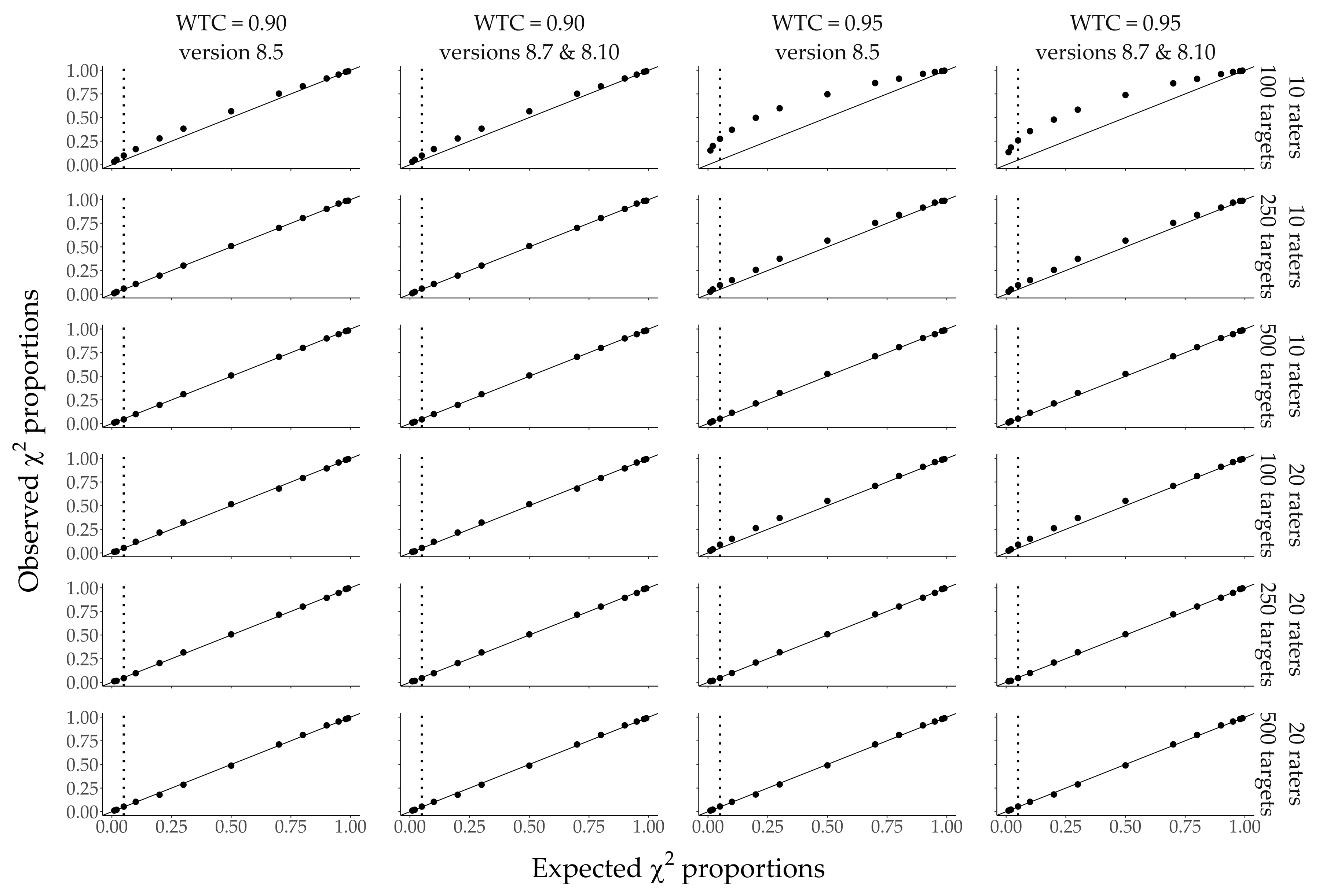
Figure 4, Figure 5 and Figure 6 display P-P plots with the simulated vs. expected proportions of χ 2 values exceeding theoretical quantiles of the corresponding theoretical χ 2 distribution in simulations applying the first model (Figure 1). It is important to note that the simulated and expected proportions refer to the right tail of the χ 2 distribution. That means, for example, that the value 0.05 is the 0.95 quantile of the χ 2 distribution, the value 0.10 is the 0.90 quantile, etc. Figure 4 and Figure 5 cover conditions with few (two or five) raters and low (Figure 4, WTC = 0.60 or 0.80) vs. high WTC (Figure 5, WTC = 0.90 or 0.95). Figure 6 covers conditions with more (10 or 20) raters and a high WTC. The plot for more (10 and 20) raters and low WTC (0.60 or 0.80) is displayed in Appendix A (Figure A2); as for those conditions, the observed and expected proportions were (almost) identical across all target conditions and Mplus versions.
As seen in Figure 4, Figure 5 and Figure 6, simulated proportions of χ 2 values exceeding other theoretical quantiles than the 0.05 quantiles (i.e., the rejection rates in Table 4) also only differed marginally between the old and new Mplus versions. Just as for the rejection rates, as the (other) values displayed in the P-P plots did not differ at all between the Mplus version in which the new correction was first implemented (version 8.7) and the most recent version (8.10); they are presented in shared columns.
For the first model, given a WTC of 0.60, the first condition to yield an approximately correct χ 2 distribution was the condition with two raters and 500 targets (see Figure 4). While in conditions with fewer targets (100 or 250), the simulated χ 2 values had a notable upward bias, all conditions with at least five raters and any number of targets yielded very close approximations of the corresponding χ 2 distributions. In conditions with WTC of 0.80, more units were necessary for a good approximation. In those conditions, while five raters and 100 targets only led to an approximately correct distribution, five raters and 250 targets led to a very good approximation. With increasing WTC, the number of units necessary for a good approximation of the theoretical χ 2 distribution increased further (see Figure 5 and Figure 6). With WTC of 0.90, while an approximately correct distribution was given in conditions with five raters and 350 targets, a very good approximation was attained in conditions with at least five raters and 500 targets. With WTC of 0.95, at least 10 raters and 250 targets were necessary for a very good approximation.
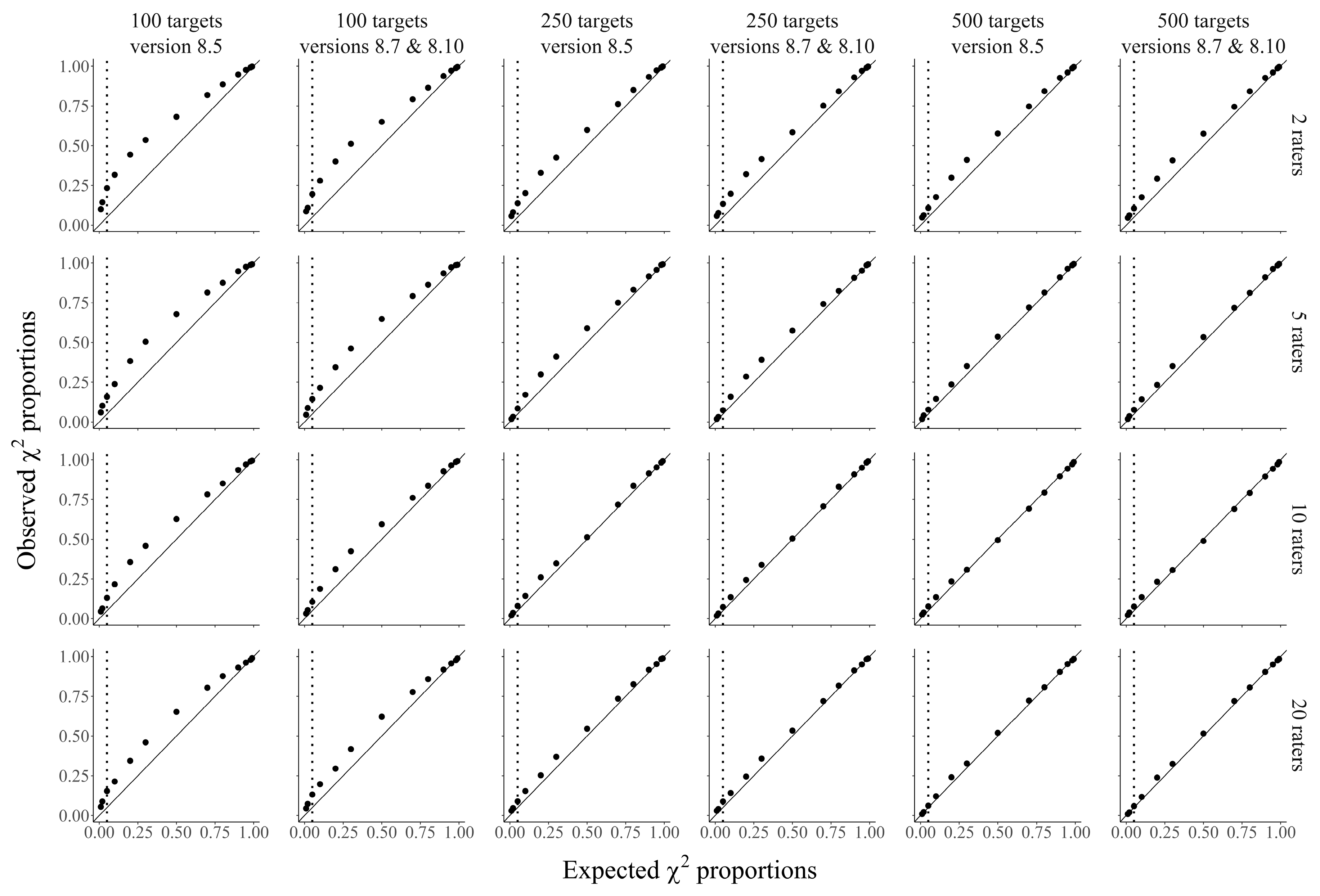
Figure 7 and Figure 8 display P-P plots with the simulated vs. expected proportions of χ 2 values exceeding theoretical quantiles of the corresponding theoretical χ 2 distribution in simulations applying the second (Figure 2) and third model (Figure 3), respectively.
In the model with unidimensional traits and interchangeable raters only (Figure 2), all WTC were one. In simulations applying this model, as compared to the model with heterogenous trait factors (Figure 1), more differences occurred between Mplus versions with the old (8.5) and new correction factors (8.7 and 8.10, see Figure 7). Especially in conditions with 100 targets and at least five raters, the new correction factor led to better approximations of χ 2 distributions for the upper tails of the distributions, where rejections happen. In the condition with 100 targets and two raters, the new correction factor also led to a small improvement, but the simulated test statistics were still clearly overestimated in the lower part of the distribution. Also, the new correction factor led to a downward bias in the upper parts of the distributions in conditions with at least five raters. In conditions with 250 and 500 targets, the simulated values were much closer to the expected ones than in those with 100 targets, and the new correction factor further enhanced the approximation, but only slightly. In the most recent Mplus version, five raters were sufficient for a good approximation of the theoretical χ 2 distributions across the four different target conditions. Given 500 targets, the distributions were also fairly well approximated with only two raters.
As seen in Figure 8, in simulations applying the model with a combination of interchangeable and structurally different raters (Figure 3), the new correction factor only led to very small improvements. In the third, most complex model, very good approximations of the expected quantiles could be attained in conditions with at least 250 targets and 10 raters or 500 targets and 5 raters. In conditions with fewer units, the simulated χ 2 values had a visible upward bias.
Differences between the χ 2 values in the old Mplus version without the correction factor (8.5) and the two versions with the new correction factor (8.7 and 8.10) were largest in conditions with unidimensional trait factors (WTC = 1) only (see Figure 7). Within the model with heterogenous trait factors, differences between the old and new Mplus versions were not bigger for larger WTC (e.g., 0.95 and 0.90; Figure 5 and Figure 6) than for smaller WTC (e.g., 0.80 and 0.60; Figure 4) but rather small in all conditions. In the most complex model with a combination of structurally different and interchangeable raters, differences between Mplus versions were also rather small (Figure 8).

3.3. RMSEA and CFI

Just like the χ 2 test of model fit values, the mean RMSEA and CFI values did not differ between Mplus versions 8.7 and 8.10. However, differences between version 8.5 and the more recent versions were also very small.
Please note that the following two paragraphs refer to mean values across replications instead of the fit indices’ distributions. This is only a rough exploration, and more complex analyses considering their distributions within simulation conditions are necessary to reliably derive sample size requirements for correct CFI and RMSEA in similar models (also see Section 4.3).
Across all models, conditions, and Mplus versions, mean CFI were very close to one. In conditions applying the two models with unidimensional trait factors (models in Figure 2 and Figure 3), all mean CFI were 0.97, so based on the mean CFI across replications, there were no type-I errors. In the model with heterogenous trait factors (model in Figure 1), based on the mean CFI, three conditions led to type-I errors: those with two raters, 100 targets, and WTC of 0.80, 0.90, and 0.95. The mean CFI in these conditions were 0.965 (SD = 0.078), 0.944 (SD = 0.123), and 0.934 (SD = 0.147), respectively, in the more recent Mplus versions and slightly lower with 0.962 (SD = 0.084), 0.939 (SD = 0.130), and 0.927 (SD = 0.176), respectively, in version 8.5.
A similar pattern occurred for the mean RMSEA: no type-I errors occurred based on the mean RMSEA when applying the rule RMSEA 0.05 for the models with unidimensional trait factors (models in Figure 2 and Figure 3). In conditions with heterogenous trait factors (Figure 1), there were seven conditions in which the mean RMSEA across replications led to a type-I error:
  • All conditions with 100 targets and two raters, which had mean RMSEA of 0.066 (SD = 0.095), 0.098 (SD = 0.123), 0.125 (SD = 0.143), and 0.139 (SD = 0.193) for the lowest to highest WTC in the more recent Mplus versions (8.7 and 8.10) and the slightly lower means of 0.065 (SD = 0.058), 0.097 (SD = 0.091), 0.124 (SD = 0.134), and 0.132 (SD = 0.191) in Mplus version 8.5;
  • The condition with 100 targets, five raters, and a WTC of 0.95, which had a mean RMSEA of 0.051 (SD = 0.044) in the more recent and of 0.068 (SD = 0.152) in the older version;
  • The conditions with 250 targets, two raters, and WTC of 0.90 and 0.95, which had mean RMSEA of 0.055 (SD = 0.048) and 0.072 (SD = 0.070), respectively, in Mplus versions 8.7 and 8.10 and of 0.055 (SD = 0.050) and 0.076 (SD = 0.099), respectively, in version 8.5.
Apart from those seven conditions, the mean RMSEA across 1000 replications in all conditions led to accepting the correctly specified models.

4. Discussion

The present simulation study was conducted to (1) evaluate whether the new correction implemented in Mplus version 8.7 sufficiently corrects the χ 2 goodness-of-fit test statistic for the MLR estimator in conditions with an increasing risk of problematic parameters in three different two-level CFA-MTMM models and to (2) identify requirements pertaining to sample sizes on both levels as well as within-trait correlations (WTC) for the χ 2 test to work as intended for those models. More precisely, as previous simulation studies have shown that the Mplus default estimator until version 8.6 results in inflated type-I error rates for models in which the level-2 residuals are fixed to zero by users—a situation quite common in MCFA-MTMM models—simulation studies with respect to two models of this type have been conducted and reported to figure out whether this problem is cured in version 8.7. Moreover, as parameters that are potentially estimated to values outside the admissible parameter space in unconstrained MLR estimation, WTC were varied in a model with heterogenous trait factors to approach one in four steps (0.60, 0.80, 0.90, and 0.95) and to finally reach one in a model with unidimensional trait factors.
As MCFA essentially always includes goodness-of-fit evaluations and as likelihood-based model fit evaluation is very popular, the present study’s results are relevant for all applied researchers conducting MCFA with multiple factors (as correlations between those factors can vary) in Mplus (and possibly other software which includes a test statistic similar to the Yuan-Bentler T 2 * test statistic [15]), as they might wonder whether and under which circumstances the p-value of their χ 2 goodness-of-fit test can be trusted. Especially researchers applying MCFA-MTMM can profit from the sample size requirements derived in our simulation study, as their models are expected to be most similar to ours (for examples of applications, see, e.g., Danay and Ziegler [28], Konold [29], Konold and Sanders [30], the studies listed in Eid et al. [11] and Geiser and Simmons [31]). Researchers applying (other) MCFA models with multiple factors might use the instructions in the OSF project linked in the present study’s data availability statement. The project includes a folder (“Instructions on tailored Monte Carlo simulations”) with user-friendly instructions on how to run Monte Carlo simulations tailored to modeling conditions other than those included in the present study.

4.1. The Correction Factor in MCFA-MTMM Modeling

The first aim of the present study was to find out whether the new correction factor sufficiently corrects the χ 2 test statistics in conditions with a large proportion of potentially problematic parameters. Investigating P-P plots which contrast the test statistics’ distributions in the Mplus versions prior to vs. after the implementation of the new correction factor, we found that the proportion of problematic parameters was only large enough for the correction factor to visibly influence the distributions in conditions in which all WTC were one and all level-2 residual variances were fixed to 0 (i.e., in the model with unidimensional trait factors and interchangeable raters only). Applying this model, the correction factor did correct the lower parts of the distributions slightly in conditions with 100 targets. However, in conditions with 100 targets and at least five raters, the new correction also led to underestimated values in the upper parts of the distributions. In most conditions with WTC of 0.95 or lower, the correction factor did not influence the χ 2 values much, which might be due to the low proportion of problematic parameters in these conditions. We assumed that the implementation of the new correction factor has a bigger impact on the χ 2 test values in conditions with a larger proportion of potentially problematic parameters than in conditions with few problematic parameters, as this was announced by Asparouhov and Muthén [9] when implementing the new correction factor. This assumption was confirmed, as the implementation had a bigger influence on the rejection rates and distributions of the simulated test statistics, i.e., went along with larger differences in the rejection rates between the Mplus versions prior to and after the implementation of the new correction, in conditions with unidimensional trait factors (many WTC in the estimated models close to one) than in models with heterogeneous trait factors.

4.2. Sample Size Requirements

The second aim of the present study was to identify requirements pertaining to sample sizes on both levels as well as WTC for the χ 2 test to work as intended for three different two-level CFA-MTMM models. We varied the number of between-level units (100, 250, 500) as well as within-level units (2, 5, 10, 20) and found that across all models, the test statistics performed best in conditions with large sample sizes on both levels. For the model with heterogenous trait factors, interestingly, the test statistics also performed notably better in conditions with smaller WTC. In other words, rejection rates and the test statistics’ distributions increasingly diverged from the nominal alpha level and the expected χ 2 distribution with decreasing sample sizes on both levels, as well as increasing WTC. As this pattern occurred in Mplus versions with and without the new correction factor, the phenomenon of more type-I errors occurring in conditions with larger WTC cannot be traced back to those WTC being estimated to parameters outside the admissible space (values above one).
In many conditions simulated in the present study, the finite samples were not large enough for the asymptotic properties of the simulated test statistics to manifest. For the model with heterogenous trait factors, rejection rates in the most recent Mplus version turned out to be adequate in conditions with total sample sizes of 1000, 2000 to 2500, and 5000 for WTC of 0.60 to 0.80, 0.90, and 0.95, respectively. Interestingly, different combinations of targets and raters that yielded the same total sample sizes differed in their rejection rates. Overall, conditions with fewer raters of more targets had higher rejection rates than conditions with more raters of few targets. Thus, study designs with more raters of few targets could yield correct rejection rates at lower total sample sizes than designs with few raters of more targets. For the model with unidimensional trait factors and interchangeable raters only, rejection rates were only adequate in conditions with 100 targets and 10 or 20 raters, and the condition with 500 targets and 20 raters. However, in all conditions with 500 targets, the model did not converge in almost 50% of the replications. For the model combining interchangeable and structurally different raters, adequate rejection rates were only attained in conditions with 250 targets and 5 or 10 raters, and in the condition with 500 targets and 20 raters.
The results concerning rejection rates and distributions as well as nonconvergence and warning messages, were identical in Mplus version 8.7, in which the new correction factor was implemented, and version 8.10. Thus, we verified that all results attained in the present study are applicable to the most recent Mplus version.
In the present study’s simulation conditions, across Mplus versions, two within-level units were often not enough for the test statistics to follow a χ 2 distribution. For the models with unidimensional trait factors, conditions with two within-level units also led to estimation problems. In those conditions, the estimation reached a saddle point or a point where the observed and expected information matrices did not match in 30 to 75% of the replications. The finding that two within-level units are often not enough for the MLR estimator to yield correct rejection rates in sample size conditions, which might be expected in MCFA-MTMM analyses, is in line with the study conducted by Koch et al. [17], who also found an upward bias in conditions with two within-level units and 350 between-level units for more complex MCFA-MTMM models [17]. However, models with two within-level units might yield correct rejection rates in conditions with more between-level units than simulated in the present study, for instance, about 1000 and 2500 for WTC of 0.90 and 0.95, respectively. This has to be analyzed in future Monte Carlo simulation studies. The present study could also replicate the finding reported by Asparouhov and Muthén [9] that the MLR estimator yields correct rejection rates given 20 within-level units and 100 between-level units for relatively simple two-level factor models. This finding was extended to two somewhat more complex models (the two models with interchangeable raters only) and to fewer (down to 10) within-level units in the present study (given WTC were 0.60, 0.80, or 1). However, in models with unidimensional trait factors, the rejection rates were inflated in most conditions, even with larger sample sizes on the between-level (e.g., 250 or 500 raters). Additionally, the present simulation study is the first to reveal that the upward bias in the χ 2 test statistics that is present for the MLR estimator in Mplus not only depends on sample sizes on both levels (small samples leading to a larger upward bias) but also on model complexity (more complex models with more indicators leading to a larger upward bias) and WTC (larger WTC leading to a larger upward bias). We also discovered that in a model with heterogenous trait factors, larger samples could compensate for higher WTC and lower WTC could partly compensate for smaller samples. The χ 2 test’s general tendency to reject too many correctly specified models with growing model complexity is in line with existing work on different (non-robust as well as robust) χ 2 goodness-of-fit test statistics [32,33,34,35,36,37,38]. A simulation study conducted by Shi et al. [38] indicates that the numbers of observed variables, as well as estimated parameters, seem to be particularly important contributing factors to the inflated rejection rates.
Several simulation studies using the (non-robust) ML estimator found a downward bias in χ 2 distributions [3,14,16,18]. The simulation study conducted by Jak et al. [8] also included conditions, e.g., correctly specified models with 100 between-level units and 20 within-level units, in which the (non-robust) ML estimator had very low rejection rates but performed better than the MLR estimator, which led to overestimated rejection rates in the same conditions. Interestingly, with small enough WTC, this downward bias can disappear, just like the upward bias that is present when using the MLR estimator can disappear with smaller WTC. Eßer et al. [19] applied the ML estimator, included small sample sizes (down to 2 within-level units and 50 between-level units), and set all WTC to 0.85. Under these conditions, the χ 2 test statistics were unbiased. Likewise, combining the ML estimator with down to 2 within-level units, 100 between-level units, and a WTC of 0.80 led to unbiased distributions in the study conducted by Ulitzsch et al. [14]. This finding is particularly interesting as it indicates that the χ 2 test in (non-robust) ML estimation can be unbiased in conditions in which one might expect that it would not, that is, conditions in which data have missing values (unbalanced designs) and few raters on the within level, given correlations within heterogenous trait factors are small enough. Under these conditions (e.g., 2 to 5within-level units, 100 between-level units, and WTC of 0.60 to 0.80), the ML estimator could even perform better than the MLR estimator (see Ulitzsch et al. [14], who reported rejection rates in Mplus version 7.3 for those conditions with and without missings).

4.3. RMSEA and CFI

Due to its well-known dependency on sample size and as it only tests the hypothesis of exact fit, some researchers tend to rely on other fit statistics more than on the χ 2 test when evaluating model fit [39,40]. However, the χ 2 test statistic is also often used for nested model comparisons [41] and the calculation of other model fit statistics like the CFI and the RMSEA [10]. Due to their dependency on the χ 2 goodness-of-fit test, our study also explored the performance of RMSEA and CFI in all simulated conditions. Based on the mean RMSEA and CFI values, when following the rules of thumb for good model fit RMSEA 0.05 and CFI 0.97, only a few type-I errors occurred, all of them in conditions with heterogenous trait factors. The errors tended to occur in conditions with smaller sample sizes and larger WTC, which indicates that the statistical performance of RMSEA and CFI values, just like χ 2 values, could also be affected by the interplay of small sample sizes and high WTC when fitting MCFA-MTMM models. However, reliably deriving sample size requirements for CFI and RMSEA in similar models would require scrutinizing their distributions instead of only inspecting their mean values across replications. Using the Mplus .out files to evaluate the performance of simulated CFI and RMSEA values is a bit more complicated, as the distributions underlying the RMSEA and CFI values are assumed to be normal in Mplus [7] (p. 471), which is usually false [42]. Their performance can instead be evaluated with external Monte Carlo simulations [7] (p. 469). Comparing distributions of simulated CFI and RMSEA values for multilevel factor models using the MLR estimator to their theoretically expected distributions was, therefore, outside the scope of this study but could be an interesting idea for future research.

4.4. Limitations and Future Directions

As Feinberg and Rubright put it, “In some cases, the extent to which findings based on simulated data generalize to practice will depend on how well the simulated data conform to the empirical data that arise in practice” [43] (p. 37). On that note, there are some aspects of the data simulated in our study that might be unrealistic in practical applications.
Firstly, in the population model, all factor loadings were set equal, all indicators were chosen to have the same reliabilities, all indicators pertaining to interchangeable raters had the same consistency, and the correlations between trait as well as method factors were fixed to the same values. Our study showed that sample size requirements for the χ 2 test depend on WTC. Similarly, other values that were fixed in the population model in our study might also influence the test statistic’s performance. Future studies might, therefore, also vary those values (factor loadings, reliabilities, consistency [ICC]/method specificity [low ICC could also lead to estimation problems [16]], and correlations between method and trait factors pertaining to different traits [between-trait correlations]) to explore their influence on likelihood-based test statistics applied to MCFA models.
Secondly, our simulation did not contain conditions with missing values. It should be noted that the requirements pertaining to sample sizes and WTC discovered in our study might not be conferrable to data with missing values. Applying non-robust (FI)ML estimation in Mplus, within their studies, Ulitzsch et al. [14] and Eßer et al. [19] did not find a notable influence of missings vs. no missings on the simulated test statistics‘ distributions. However, to our knowledge, so far, nobody has tested the influence of missing values on the performance of MLR-based goodness-of-fit test statistics for MCFA models. Recently, Shi et al. compared the performance of model fit statistics for latent growth curve models with non-normal data including missing values using different robust and non-robust ML estimators (ML, MLM, MLR, MLMV) in Mplus [44]. They found that rejection rates for the χ 2 test were inflated for all estimators, and that rejection rates differed significantly between sample size conditions, the number of time occasions, and three interactions between the variables manipulated in the study [44]. Overall, they were most accurate when selecting the MLMV estimator, but as the MLMV estimator requires complete data, it was combined with listwise deletion [44]. Similarly, Savalei and Falk [45] found inflated rejection rates for robust FIML estimation for single-level factor models with non-normal data in EQS [46]. Jia [47] recently investigated the performance of two different pooled χ 2 test statistics applied to single-level models, data with varying degrees of non-normality, two kinds of multiple imputation, and different missing data mechanisms in the R package semTools [48]. The MLR estimator went along with inflated rejection rates and, overall, performed worse than the MLM and the MLMV estimator [47]. Hence, investigating different fit statistics’ performance with missing data for MCFA (instead of single-level) models using different robust estimators in Mplus or other software might still be an interesting idea for future research.
Thirdly, we used the known population parameters as starting values in all estimated models. This represents the best-case scenario for model estimation, and in practice, if researchers use starting values, they are likely not as accurate as in our simulation. The proportions of warning messages displayed in Table 2 and Table 3 might be higher with less accurate or no starting values. However, the pattern of rejection rates of the χ 2 test can be expected to hold in practice (when using other or the default starting values).
Additionally, some other notes are to be made on the boundaries of the present study’s results. We only tested the performance of the χ 2 goodness-of-fit test statistic for correctly specified models. Thus, the present study does not allow for reporting results on false negative results or the power to detect model misfit. For approaches to study model misfit, see, e.g., Maydeu-Olivares [49]; for a recent simulation study on estimators’ power to detect misfit in (ordinal) MCFA in Mplus, see Padgett and Morgan [50]. A simulation study conducted by Hsu et al. [40] found that the power to detect different kinds of misspecification in multilevel models with the χ 2 goodness-of-fit test depends on the number of between-level units and ICC [40]. Expanding on those findings, future studies could test the χ 2 test statistic’s power to detect different kinds of misspecification in more complex MCFA-MTMM models with heterogenous or simply more trait factors, models with combinations of interchangeable and structurally different methods, and/or longitudinal models. Also, our study focused on the “standard” χ 2 test of model fit, which evaluates the goodness-of-fit for the entire model, i.e., jointly for the between- and the within-level. In multilevel models, this test is expected to be dominated by misspecifications on the within-level [40,51]. In the past few years, some studies have also investigated the performance of level-specific fit indices for multilevel models [51,52,53,54]. In future studies, investigations on the performance of level-specific fit indices could also be extended to more complex MCFA-MTMM models. Finally, the present study only included continuous indicators. In future studies, existing research on the performance of model fit statistics for CFA-MTMM models with categorical observed variables [55,56,57] might also be extended to more complex CFA-MTMM models, e.g., for nested or longitudinal data or a larger number of traits.

5. Conclusions

Researchers evaluating the fit of MCFA-MTMM models, and multilevel factor models in general, should be aware that the χ 2 goodness-of-fit test can yield an increased probability of type-I errors. The certainty with which the test statistic can be trusted can depend on many different factors. Variables that might influence the test statistics’ performance include sample sizes on both levels, correlations within trait factors, the chosen estimator (robust vs. non-robust), software, the presence of missing data, non-normality of the indicators, intraclass correlations and reliabilities, model complexity, as well as the size of other model parameters. Table 7 contains an overview of sample sizes that are likely sufficient for the χ 2 test to yield correct rejection rates when applying the MLR estimator in Mplus versions starting with version 8.7 for relatively simple and correctly specified MCFA models with two traits. Models with unidimensional trait factors, i.e., within-trait correlations equal to one, tend to require larger sample sizes than those with heterogenous trait factors. However, applying those models, in some cases, larger sample sizes also come along with a slightly higher risk of type-I errors than smaller ones. Thus, simple rules of thumb pertaining to sample size requirements for likelihood-based goodness-of-fit test statistics should be regarded with due caution, especially for models with unidimensional trait factors.
In studies with data that are sufficiently similar to the data simulated in the present study, similar sample size requirements can be expected. Therefore, when planning studies that include overall model fit evaluations of simple MCFA-MTMM or similar MCFA models, researchers can roughly estimate how many participants they need for the χ 2 test to work as intended by looking for the model and WTC which are most similar to their applied model(s) in Table 7, and aim for sample sizes that yielded correct rejection rates in the present study. However, for other conditions, e.g., more complex models, other estimators, data with missing values, categorical indicators, other ICC, other reliabilities, etc., sample size requirements might differ. The idea to simply ignore χ 2 values and rely on other fit statistics instead can also cause false conclusions as some of these coefficients, like CFI and RMSEA, are based on the χ 2 test statistic. Therefore, they might be affected by the same variables. When in doubt, researchers might consider calculating required sample sizes tailored to their specific modeling conditions. Mplus .out files of Monte Carlo simulations can easily be inspected to find out whether specific sample sizes are likely to yield correct rejection rates for the χ 2 test under the expected conditions [7] (p. 470). The OSF project linked in the data availability statement includes a folder (“Instructions on tailored Monte Carlo simulations”) with user-friendly instructions on how to run Monte Carlo simulations tailored to other modeling conditions than those included in the present study.

Author Contributions

Conceptualization, M.L.H., F.T. and M.E.; methodology, M.L.H. and M.E.; software, M.L.H.; validation, F.T. and M.E.; formal analysis, M.L.H.; resources, M.E.; data curation, M.L.H.; writing—original draft preparation, M.L.H.; writing—review and editing, M.E. and F.T.; visualization, M.L.H.; supervision, M.E.; project administration, M.L.H. All authors have read and agreed to the published version of the manuscript.

Funding

We acknowledge support by the Open Access Publication Fund of the Freie Universität Berlin.

Institutional Review Board Statement

Not applicable.

Informed Consent Statement

Not applicable.

Data Availability Statement

An Open Science Framework (OSF) project which can be accessed via https://osf.io/s5vtr/ (accessed on 21 March 2024) includes all files allowing for an exact replication of the study in the folder “Files to replicate the simulation study”: R scripts for calculating parameter and starting values (Calculating_template_values.R), .rtf files with information on the R versions, template files (.txt), Mplus .inp and .out files, and R scripts for running the models and evaluating the .out files (MplusAutomation_Run.R and Evaluation_Plots_and_Tables.R, respectively). Additionally, it includes some user-friendly instructions on how to run Monte Carlo simulations tailored to other modeling conditions than those included in the present study (“Instructions on tailored Monte Carlo simulations”).

Acknowledgments

We want to thank Esther Ulitzsch for sharing relevant Mplus files of her article from 2016 with us. We would also like to thank Claudia Crayen and Mario Lawes for their assistance in running the simulation, Claudia Crayen for her assistance in creating the iterators for the template files, and the reviewers for their helpful comments and suggestions.

Conflicts of Interest

The authors declare no conflict of interest.

Abbreviations

The following abbreviations are used in the manuscript:
CFAconfirmatory factor analysis/analyses
CFIcomparative fit index/indices
ICCintraclass correlation(s)
LRTlikelihood-ratio test(s)
MCFAmultilevel confirmatory factor analysis/analyses
MLmaximum likelihood
MLRrobust maximum likelihood
MTMMmultitrait-multimethod
P-P plotprobability-probability plot
RMSEAroot mean square error(s) of approximation
WTCwithin-trait correlation(s)

Appendix A

Table A1. Proportions of Mplus warning messages for the first model with interchangeable raters only and heterogenous trait factors and all conditions.
Heterogenous   Trait   Factors   ( WTC   1)
nt = 100nt = 250nt = 500
nrWTCTotalSPNC Ψ TotalSPNC Ψ TotalSPNC Ψ
20.600.0020.00200.0020.0060.00600.0060000
0.8000000.0050.00500.0050.0050.00500.004
0.9000000.0010.00100.0010.0250.0040.0210.004
0.95000000000.11200.1120
50.600.0010.00100.00100000000
0.80000000000000
0.900.0020.00200.0020.0070.00600.0070000
0.950.0010.00100.0010.0010.00100.0010.0040.00300.004
100.60000000000000
0.80000000000000
0.900.0020.00200.00200000000
0.950.0010.00100.0010.0030.00200.0030.0010.00100.001
200.60000000000000
0.80000000000000
0.90000000000000
0.950.0020.00100.00200000000
Note. As Table 2 only contains conditions with 500 targets and up to 10 raters, this table includes all simulated conditions for the first model, in which within-trait correlations (WTC) were varied. Proportions of warning messages per 1000 replications in Mplus are shown. Values above 0.05 are bold-faced. nt = number of targets (Level 2 units); nr = number of raters (Level 1 units); Total = replications with warnings; SP = “The estimation has reached a saddle point or a point where the observed and the expected information matrices do not match”; NC = “The H 1 model estimation did not converge”; Ψ = “The latent variable covariance matrix [ Ψ ] is not positive definite”. Values above 0.05 are bold-faced.
Figure A1. Path diagram displaying how population values were set in the three models. Arrows indicate calculations based on previously set values. Also see “Calculating_template_values.R”, the corresponding R script in the OSF project to this article.
Psycholint 06 00029 g0a1
Figure A2. P-P Plots with expected vs. observed proportions of χ 2 values for the first model (model with interchangeable raters only and heterogeneous traits, see Figure 1) in conditions with 10 and 20 within-level units (raters) and correlations within traits (WTC) of 0.60 and 0.80. The nominal alpha level of 0.05 is marked by vertical dotted lines.
Psycholint 06 00029 g0a2

References

  1. Campbell, D.T.; Fiske, D.W. Convergent and discriminant validation by the multitrait-multimethod matrix. Psychol. Bull. 1959, 56, 81–105. [Google Scholar] [CrossRef] [PubMed]
  2. Koch, T.; Eid, M.; Lochner, K. Multitrait-multimethod-analysis. In The Wiley Handbook of Psychometric Testing: A Multidisciplinary Reference on Survey, Scale, and Test Development; Irwing, P., Booth, T., Hughes, D.J., Eds.; Wiley Blackwell: Hoboken, NJ, USA, 2018; pp. 781–846. [Google Scholar] [CrossRef]
  3. Koch, T.; Schultze, M.; Eid, M.; Geiser, C. A longitudinal multilevel CFA-MTMM model for interchangeable and structurally different methods. Front. Psychol. 2014, 5, 76604. [Google Scholar] [CrossRef] [PubMed]
  4. Eid, M.; Nussbeck, F.W.; Geiser, C.; Cole, D.A.; Gollwitzer, M.; Lischetzke, T. Structural equation modeling of multitrait-multimethod data: Different models for different types of methods. Psychol. Methods 2008, 13, 230–253. [Google Scholar] [CrossRef] [PubMed]
  5. Kenny, D.A. The multitrait-multimethod matrix: Design, analysis, and conceptual issues. In Personality Research, Methods, and Theory: A Festschrift Honoring Donald W. Fiske; Shrout, P.E., Fiske, S.T., Eds.; Lawrence Erlbaum Associates: Mahwah, NJ, USA, 1995; pp. 111–124. [Google Scholar]
  6. Kelloway, E.K. Using Mplus for Structural Equation Modeling: A Researcher’s Guide, 2nd ed.; SAGE Publications, Inc.: Los Angeles, CA, USA, 2015. [Google Scholar] [CrossRef]
  7. Muthén, L.K.; Muthén, B.O. Mplus User’s Guide, 8th ed.; Muthén & Muthén: Los Angeles, CA, USA, 2017. [Google Scholar]
  8. Jak, S.; Jorgensen, T.D.; Rosseel, Y. Evaluating cluster-level factor models with lavaan and Mplus. Psych 2021, 3, 134–152. [Google Scholar] [CrossRef]
  9. Asparouhov, T.; Muthén, B. Robust chi-square in extreme and boundary conditions: Comments on Jak et al. (2021). Psych 2021, 3, 542–551. [Google Scholar] [CrossRef]
  10. Muthén, B.O. Mplus Technical Appendices, 3rd ed.; Muthén & Muthén: Los Angeles, CA, USA, 2004. [Google Scholar]
  11. Eid, M.; Geiser, C.; Koch, T. Structural Equation Modeling of Multiple Rater Data; Guilford Press: New York, NY, USA, 2025; in press. [Google Scholar]
  12. Muthén, B.O. Multilevel covariance structure analysis. Sociol. Methods Res. 1994, 22, 376–398. [Google Scholar] [CrossRef]
  13. Kaplan, D.; Kim, J.-S.; Kim, S.-Y. Multilevel latent variable modeling: Current research and recent developments. In The SAGE Handbook of Quantitative Methods in Psychology; Millsap, R.E., Ed.; SAGE Publications, Inc.: London, UK, 2009; pp. 592–612. [Google Scholar] [CrossRef]
  14. Ulitzsch, E.; Holtmann, J.; Schultze, M.; Eid, M. Comparing multilevel and classical confirmatory factor analysis parameterizations of multirater data: A Monte Carlo simulation study. Struct. Equ. Model. 2017, 24, 80–103. [Google Scholar] [CrossRef]
  15. Yuan, K.-H.; Bentler, P.M. Three likelihood-based methods for mean and covariance structure analysis with nonnormal missing data. Sociol. Methodol. 2000, 30, 165–200. [Google Scholar] [CrossRef]
  16. Pornprasertmanit, S.; Lee, J.; Preacher, K.J. Ignoring clustering in confirmatory factor analysis: Some consequences for model fit and atandardized parameter estimates. Multivariate Behav. Res. 2014, 49, 518–543. [Google Scholar] [CrossRef] [PubMed]
  17. Koch, T.; Schultze, M.; Holtmann, J.; Geiser, C.; Eid, M. A multimethod latent state-trait model for structurally different and interchangeable methods. Psychometrika 2017, 82, 17–47. [Google Scholar] [CrossRef] [PubMed]
  18. Mahlke, J.; Schultze, M.; Eid, M. Analysing multisource feedback with multilevel structural equation models: Pitfalls and recommendations from a simulation study. Br. J. Math. Stat. Psychol. 2019, 72, 294–315. [Google Scholar] [CrossRef] [PubMed]
  19. Eßer, F.J.; Holtmann, J.; Eid, M. A Monte Carlo simulation study on the influence of unequal group sizes on parameter estimation in multilevel confirmatory factor analysis. Struct. Equ. Model. 2021, 28, 827–838. [Google Scholar] [CrossRef]
  20. Kim, E.S.; Yoon, M.; Wen, Y.; Luo, W.; Kwok, O. Within-level group factorial invariance with multilevel data: Multilevel factor mixture and multilevel MIMIC models. Struct. Equ. Model. 2015, 22, 603–616. [Google Scholar] [CrossRef]
  21. Kim, E.S.; Kwok, O.; Yoon, M. Testing factorial invariance in multilevel data: A Monte Carlo study. Struct. Equ. Model. 2012, 19, 250–267. [Google Scholar] [CrossRef]
  22. Hallquist, M.N.; Wiley, J.F. MplusAutomation: An R package for facilitating large-scale latent variable analyses in Mplus. Struct. Equ. Model. 2018, 25, 621–638. [Google Scholar] [CrossRef]
  23. R Core Team. R: A Language for Statistical Computing; R Foundation for Statistical Computing: Vienna, Austria, 2022; Available online: https://www.R-project.org/ (accessed on 11 January 2024).
  24. Posit Team. RStudio: Integrated Development Environment for R; Posit Software; PBC: Boston, MA, USA, 2023; Available online: http://www.posit.co/ (accessed on 11 January 2024).
  25. Wickham, H.; Averick, M.; Bryan, J.; Chang, W.; McGowan, L.; François, R.; Grolemund, G.; Hayes, A.; Henry, L.; Hester, J.; et al. Welcome to the tidyverse. J. Open Source Softw. 2019, 4, 1686. [Google Scholar] [CrossRef]
  26. Bradley, J.V. Robustness? Br. J. Math. Stat. Psychol. 1978, 31, 144–152. [Google Scholar] [CrossRef]
  27. Schermelleh-Engel, K.; Moosbrugger, H.; Müller, H. Evaluating the fit of structural equation models: Tests of significance and descriptive goodness-of-fit measures. Psychol. Methods 2003, 8, 23–74. [Google Scholar]
  28. Danay, E.; Ziegler, M. Is there really a single factor of personality? A multirater approach to the apex of personality. J. Res. Pers. 2011, 45, 560–567. [Google Scholar] [CrossRef]
  29. Konold, T. A multilevel MTMM approach to estimating the influences of contextual factors on trait and informant-based method effects in assessments of school climate. J. Psychoeduc. Assess. 2018, 36, 464–476. [Google Scholar] [CrossRef]
  30. Konold, T.; Sanders, E.A. The nature of rater effects and differences in multilevel MTMM latent variable models. Meas. Interdiscip. Res. Perspect. 2020, 18, 177–195. [Google Scholar] [CrossRef]
  31. Geiser, C.; Simmons, T.G. Do method effects generalize across traits (and what if they don’t)? J. Pers. 2021, 89, 382–401. [Google Scholar] [CrossRef] [PubMed]
  32. Herzog, W.; Boomsma, A.; Reinecke, S. The model-size effect on traditional and modified tests of covariance structures. Struct. Equ. Model. 2007, 14, 361–390. [Google Scholar] [CrossRef]
  33. Hayakawa, K. Corrected goodness-of-fit test in covariance structure analysis. Psychol. Methods 2019, 24, 371–389. [Google Scholar] [CrossRef]
  34. Hau, K.-T.; Marsh, H.W. The use of item parcels in structural equation modelling: Non-normal data and small sample sizes. Br. J. Stat. Psychol. 2004, 57, 327–351. [Google Scholar] [CrossRef] [PubMed]
  35. Moshagen, M. The model size effect in SEM: Inflated goodness-of-fit statistics are due to the size of the covariance matrix. Struct. Equ. Model. 2012, 19, 86–98. [Google Scholar] [CrossRef]
  36. Zheng, B.Q.; Valente, M.J. Evaluation of goodness-of-fit tests in random intercept cross-lagged panel model: Implications for small samples. Struct. Equ. Model. 2023, 30, 604–617. [Google Scholar] [CrossRef]
  37. Arruda, E.H.; Bentler, P.M. A regularized GLS for structural equation modeling. Struct. Equ. Model. 2017, 24, 657–665. [Google Scholar] [CrossRef]
  38. Shi, D.; Lee, T.; Terry, R.A. Revisiting the model size effect in structural equation modeling. Struct. Equ. Model. 2018, 25, 21–40. [Google Scholar] [CrossRef]
  39. Brown, T.A. Confirmatory Factor Analysis for Applied Research, 2nd ed.; Guilford Press: New York, NY, USA, 2015. [Google Scholar]
  40. Hsu, H.-Y.; Kwok, O.; Lin, H., Jr.; Acosta, S. Detecting misspecified multilevel structural equation models with common fit indices: A Monte Carlo study. Multivariate Behav. Res. 2015, 50, 197–215. [Google Scholar] [CrossRef] [PubMed]
  41. Chi-Square Difference Testing Using the Satorra-Bentler Scaled Chi-Square. Available online: https://www.statmodel.com/chidiff.shtml (accessed on 19 June 2023).
  42. Rigdon, E.E. CFI versus RMSEA: A comparison of two fit indexes for structural equation modeling. Struct. Equ. Model. 1996, 3, 369–379. [Google Scholar] [CrossRef]
  43. Feinberg, R.A.; Rubright, J.D. Conducting simulation studies in psychometrics. Educ. Meas. 2016, 35, 36–49. [Google Scholar] [CrossRef]
  44. Shi, D.; DiStefano, C.; Zheng, X.; Liu, R.; Jiang, Z. Fitting latent growth models with small sample sizes and non-normal missing data. Int. J. Behav. Dev. 2021, 45, 179–192. [Google Scholar] [CrossRef] [PubMed]
  45. Savalei, V.; Falk, C.F. Robust two-stage approach outperforms robust full information maximum likelihood with incomplete nonnormal data. Struct. Equ. Model. 2014, 21, 280–302. [Google Scholar] [CrossRef]
  46. Bentler, P.M. EQS 6 Structural Equations Program Manual; Multivariate Software Inc.: Encino, CA, USA, 2006; Available online: http://www.econ.upf.edu/~satorra/CourseSEMVienna2010/EQSManual.pdf (accessed on 11 January 2024).
  47. Jia, F. Pooling test statistics across multiply imputed datasets for nonnormal items. Behav. Res. 2023. online ahead of print. [Google Scholar] [CrossRef]
  48. Jorgensen, T.D.; Pornprasertmanit, S.; Shoemann, A.M.; Rosseel, Y. semTools: Useful Tools for Structural Equation Modeling. R Package. 2022. Available online: https://CRAN.R-project.org/package=semTools (accessed on 21 March 2024).
  49. Maydeu-Olivares, A. Assessing the size of model misfit in structural equation models. Psychometrika 2017, 82, 533–558. [Google Scholar] [CrossRef] [PubMed]
  50. Padgett, R.N.; Morgan, G.B. Multilevel CFA with ordered categorical data: A simulation study comparing fit indices across robust estimation methods. Struct. Equ. Model. 2021, 28, 51–68. [Google Scholar] [CrossRef]
  51. Ryu, E.; West, S.G. Level-specific evaluation of model fit in multilevel structural equation modeling. Struct. Equ. Model. 2009, 16, 583–601. [Google Scholar] [CrossRef]
  52. Lee, B.; Sohn, W. Testing the performance of level-specific fit evaluation in MCFA models with different factor structures across levels. Educ. Psychol. Meas. 2022, 82, 1153–1179. [Google Scholar] [CrossRef] [PubMed]
  53. Hsu, H.-Y.; Lin, J.-H.; Kwok, O.; Acosta, S.; Willson, V. The impact of intraclass correlation on the effectiveness of level-specific fit indices in multilevel structural equation modeling: A Monte Carlo study. Educ. Psychol. Meas. 2017, 77, 5–31. [Google Scholar] [CrossRef] [PubMed]
  54. Lin, J.J.H.; Hsu, H.-Y. Investigating the performance of level-specific fit indices in multilevel confirmatory factor analysis with dichotomous indicators: A Monte Carlo study. Behav. Res. 2022, 55, 4222–4259. [Google Scholar] [CrossRef]
  55. Beauducel, A.; Herzberg, P.Y. On the performance of maximum likelihood versus means and variance adjusted weighted least squares estimation in CFA. Struct. Equ. Model. 2006, 13, 186–203. [Google Scholar] [CrossRef]
  56. Hox, J.J.; Maas, C.J.M.; Brinkhuis, M.J.S. The effect of estimation method and sample size in multilevel structural equation modeling. Stat. Neerl. 2010, 64, 157–170. [Google Scholar] [CrossRef]
  57. Depaoli, S.; Clifton, J.P. A Bayesian approach to multilevel structural equation modeling with continuous and dichotomous outcomes. Struct. Equ. Model. 2015, 22, 327–351. [Google Scholar] [CrossRef]
Figure 1. Multilevel multitrait-multimethod factor model for interchangeable raters only with heterogenous trait factors. T tik = indicator-specific trait factors; Y trik = observed variables; E trik = residual variables; M trk = rater-specific method variables; λ Mik = estimated method factor loadings; t = target (e.g., teacher); r = rater (e.g., student). The model contains two traits (clarity and time mgmt = management) and three indicators per trait. As trait factors are indicator-specific, within-trait correlations (WTC) do not equal one, and all trait factor loadings are set to one. Method factors are unidimensional within but not between traits. The first loading of each method factor is set to one for identification reasons. Figure adapted with permission from Figure 1 in Ulitzsch et al. [14].
Psycholint 06 00029 g001
Figure 2. Multilevel multitrait-multimethod factor model for interchangeable raters only with homogenous (unidimensional) trait factors. T tk = trait factors (not indicator-specific); Y trik = observed variables; E trik = residual variables; M trk = rater-specific method variables; λ Tik = estimated trait factor loadings; λ Mik = estimated method factor loadings; t = target (e.g., teacher); r = rater (e.g., student). The model contains two traits (clarity and time mgmt = management) and three indicators per trait. As trait factors are unidimensional, within-trait correlations (WTC) equal one, and only the first loading of each trait factor is set to one for identification reasons. Likewise, the first loading of each method factor is set to one. Method factors are unidimensional within but not between traits. Figure adapted with permission from Figure 1 in Ulitzsch et al. [14].
Psycholint 06 00029 g002
Figure 3. Multilevel multimethod factor model for a combination of one set of interchangeable raters, e.g., students nested in teachers, and three structurally different rater groups, e.g., teachers, students, and principals, with one unidimensional trait factor for each rater group, and three indicators per trait. TR tkj = trait-rater factors; λ TRikj = estimated trait-rater factor loadings; Y trik j and Y tik j = observed variables; E trik j = residual variables; M trkj = unique rater-specific factors; λ Mikj = estimated unique rater-specific factor loadings; t = target (e.g., teacher); r = rater (e.g., student). As trait-rater factors TR tkj on the between-level are unidimensional, within-trait correlations (WTC) for indicator-specific trait factors pertaining to interchangeable raters τ tikj equal one. The first loading of each factor is set to one for identification reasons. Figure adapted with permission from Figure 7.1 in Eid et al. [11], forthcoming Fall 2024 (Guilford Press 2025).
Psycholint 06 00029 g003
Figure 4. P-P Plots with expected vs. observed proportions of χ 2 values for the first model (model with interchangeable raters only and heterogeneous traits, see Figure 1) in conditions with two and five within-level units (raters) and correlations within traits (WTC) of 0.60 and 0.80. The nominal alpha level of 0.05 is marked by vertical dotted lines.
Psycholint 06 00029 g004
Figure 5. P-P Plots with expected vs. observed proportions of χ 2 values for the first model (model with interchangeable raters only and heterogenous traits, see Figure 1) in conditions with two and five within-level units (raters) and correlations within traits (WTC) of 0.90 and 0.95. The nominal alpha level of 0.05 is marked by vertical dotted lines.
Psycholint 06 00029 g005
Figure 6. P-P Plots with expected vs. observed proportions of χ 2 values for the first model (model with interchangeable raters only and heterogeneous traits, see Figure 1) in conditions with 10 and 20 within-level units (raters) and correlations within traits (WTC) of 0.90 and 0.95. The nominal alpha level of 0.05 is marked by vertical dotted lines.
Psycholint 06 00029 g006
Figure 7. P-P Plots with expected vs. observed proportions of χ 2 values for the second model (model with interchangeable raters only and unidimensional traits, see Figure 2). The nominal alpha level of 0.05 is marked by vertical dotted lines.
Psycholint 06 00029 g007
Figure 8. P-P Plots with expected vs. observed proportions of χ 2 values for the third model (model with a combination of interchangeable and structurally different raters, see Figure 3). The nominal alpha level of 0.05 is marked by vertical dotted lines.
Psycholint 06 00029 g008
Table 1. Previous simulations in Mplus applying MCFA models and reporting results on χ 2 .
StudyModelsnL2nL1est.ver.mis.Results
Koch et al. (2014) [3] Latent State-Combination-Of-Methods (LS-COM) model (longitudinal MCFA-MTMM)100, 250, 5002, 5, 10, 20ML6.1noSlight downward bias in χ 2 across all sample sizes, less
severe for less complex models; approx. correct rejection rates.
Pornprasertmanit et al. (2014) [16]MCFA with two factors on both levels50, 20010, 40ML7noConvergence issues and downward bias in rejection rates for low ICC (0.05) in nL2 = 200 & nL1 = 10 conditions; otherwise, approx. correct rejection rates.
Ulitzsch et al. (2017) [14]Models displayed in Figure 1 and Figure 2100, 250, 5002, 3, 5ML7.3yesDownward bias in χ 2 for models with WTC = 1 but not with lower WTC (0.6 and 0.8) across all sample sizes, with and without missings.
Koch et al. (2017) [17]Latent State-Trait Combination-Of-Methods (LST-COM) models with indicator-specific factors and one vs. two constructs350, 700, 1400, 3000 12, 5, 10, 20 1MLR5.21noMarginal upward bias in χ 2 ; Approx. correct type-I error rates for all conditions but one with nL2 = 350, nL1 = 2, and two traits.
Mahlke et al. (2019) [18]MCFA-MTMM model with two sets of interchangeable methods, a structurally different reference method, and two vs. three constructs100, 250, 4002, 4, 6, 8ML7yes 2Strong downward bias in χ 2 across all sample sizes.
Eßer et al. (2021) [19]Model displayed in Figure 150, 100, 150, 2002, 4, 7, 9 3ML8.3yesNo bias in χ 2 throughout all conditions.
Jak et al. (2021) [8]MCFA models with one construct and varied measurement invariance conditions50, 100, 20020MLR8.5noInflated type-I error rates for models with residual variances set to 0 in the population model.
Asparouhov & Muthén (2021) [9]Replication of critical models (residual variances set to zero in the population model) from Jak et al. (2021)10020MLR8.6, 8.7noInflated type-I error rates in Mplus version 8.6, adequate error rates in version 8.7.
Note. nL1 = Sample sizes on the within-level; nL2 = sample sizes on the between-level; est. = selected estimator; ver. = Mplus version; mis. = simulated missing values; approx. = approximately. This table does not stem from a systematic review and might not be exhaustive. It was mainly created to give a brief overview of previous results relevant to the present study. Although closely related, the table does not include studies on rejection rates for LRT tests on measurement invariance between groups in MCFA models like those conducted by Kim et al. [20,21], as these were not the main focus of this work. 1 Only in this study, not all nL1 and nL2 were combined, just 2 and 350, 5 and 700, 10 and 1400, and 20 and 3000. 2 This study applied a planned missingness structure with a large proportion of missing data. 3 This study included unbalanced designs. In unbalanced conditions, these nL1 are means.
Table 2. Proportions of Mplus warning messages for the first model with interchangeable raters only and heterogenous trait factors.
Heterogenous   Trait   Factors   ( WTC   1)
ntnrWTCTotalSPNC Ψ
50020.600000
0.800.0050.00500.004
0.900.0250.0040.0210.004
0.950.11200.1120
50.600000
0.800000
0.900000
0.950.0040.00300.004
100.600000
0.800000
0.900000
0.950.0010.00100.001
Note. Only for the first model, in which within-trait correlations (WTC) were varied, proportions of warning messages per 1000 replications in Mplus are shown for the conditions with 500 targets and up to 10 raters. nt = number of targets (level 2 units); nr = number of raters (level 1 units); Total = replications with warnings; SP = “The estimation has reached a saddle point or a point where the observed and the expected information matrices do not match”; NC = “The H 1 model estimation did not converge”; Ψ = “The latent variable covariance matrix [ Ψ ] is not positive definite”. Values above 0.05 are bold-faced.
Table 3. Proportions of Mplus warning messages for the second (interchangeable raters, homogenous traits) and third model (interchangeable and structurally different raters).
Homogenous   Trait   Factors   ( WTC = 1)
Model 2Model 3
ntnrTotalSPNC TotalSPNC
10020.5640.56400.0020.2920.28500.007
500000000
1000000000
2000000000
25020.6830.6830.00100.3580.35800
500000000
100.00100.00100000
200.00300.00300000
50020.8760.7520.47900.4520.4460.0120
50.49700.49800.02500.0250
100.49700.49800.02100.0210
200.48600.48800.02400.0240
Note. For each condition and only for the second and third model, proportions of warning messages per 1000 replications in Mplus are shown. nt = number of targets (level 2 units); nr = number of raters (level 1 units); Total = replications with warnings, SP = “The estimation has reached a saddle point or a point where the observed and the expected information matrices do not match”; NC = “The H 1 model estimation did not converge”; = “non-positive definite first-order derivative product matrix”. Values above 0.05 are bold-faced.
Table 4. Rejection rates based on the χ 2 test of model fit with an alpha level of 0.05 for the first model with interchangeable raters only and heterogenous trait factors.
Heterogenous   Trait   Factors   ( WTC   1)
nt = 100nt = 250nt = 500
nrWTCVersion 8.58.7 and 8.10Version 8.58.7 and 8.10Version 8.58.7 and 8.10
20.600.4390.4370.1410.1410.0640.064
0.800.6080.6130.3000.2940.1270.127
0.900.6410.6980.5670.5700.3600.359
0.950.5650.7060.6690.6880.5780.575
50.600.0860.0860.0510.0510.0530.053
0.800.1220.1210.0520.0520.0530.053
0.900.3570.3280.0960.0960.0620.062
0.950.5980.5590.3290.3250.1640.166
100.600.0680.0680.0590.0590.0430.043
0.800.0690.0690.0590.0590.0430.043
0.900.0980.0970.0590.0590.0440.044
0.950.2750.2580.0940.0940.0520.052
200.600.0520.0520.0440.0440.0540.054
0.800.0520.0520.0440.0440.0540.054
0.900.0530.0530.0440.0440.0540.054
0.950.0880.0880.0450.0450.0550.055
Note. For each condition and only for the first model, in which within-trait correlations (WTC) were varied, rejection rates based on the χ 2 test of model fit for 1000 replications are shown. nt = number of targets (Level 2 units); nr = number of raters (Level 1 units). Values above 0.075 are bold-faced.
Table 5. Comparison of rejection rates based on the χ 2 test of model fit with an alpha level of 0.05 for the first model between different sample size conditions yielding the same total N.
Heterogenous   Trait   Factors   ( WTC   1)
N = 1000N = 2500N = 5000
WTCnr = 2, nt = 500nr = 10, nt = 100nr = 5, nt = 500nr = 10, nt = 250nr = 10, nt = 500nr = 20, nt = 250
0.600.0640.0680.0530.0590.0540.044
0.800.1270.0690.0530.0590.0540.044
0.900.3590.0970.0620.0590.0540.044
0.950.5750.2580.1660.0940.0550.045
Note. For conditions yielding total sample sizes of N = 1000, 2500, and 5000 and only for the first model, in which within-trait correlations (WTC) were varied, rejection rates based on the χ 2 test of model fit for 1000 replications in the most recent Mplus version are shown. nt = number of targets (Level 2 units); nr = number of raters (Level 1 units). Values above 0.075 are bold-faced.
Table 6. Rejection rates based on the χ 2 test of model fit with an alpha level of 0.05 for the second and third model with unidimensional trait factors.
Homogenous   Trait   Factors   ( WTC = 1)
Model 2Model 3
ntnrVersion 8.58.7 and 8.10Version 8.58.7 and 8.10
10020.3240.2440.2330.196
50.1700.0970.1580.144
100.1300.0640.1320.106
200.1220.0600.1540.132
25020.1830.1650.1380.134
50.0960.0770.0850.074
100.1060.0830.0800.073
200.1000.0830.0890.088
50020.1340.1340.1080.106
50.0950.0890.0780.077
100.0870.0850.0770.076
200.0800.0700.0620.059
Note. For each condition and for the second and third model, rejection rates based on the χ 2 test of model fit for 1000 replications are shown. nt = number of targets (Level 2 units); nr = number of raters (Level 1 units). Values above 0.075 are bold-faced.
Table 7. Combinations of sample sizes and within-trait correlations likely leading to correct or incorrect statistical decisions based on the χ 2 test of model fit with an alpha level of 0.05.
nt = 100nt = 250nt = 500
WTC/nr251020251020251020
0.60!!!
0.80!!!!
0.90!!!!!!
0.95!!!!!!!!!
Note. WTC = within-trait correlations; nt = number of targets (Level 2 units); nr = number of raters (Level 1 units); ! = (inflated) rejection rates above 0.075; = (adequate) rejection rates between 0.025 and 0.075.
Disclaimer/Publisher’s Note: The statements, opinions and data contained in all publications are solely those of the individual author(s) and contributor(s) and not of MDPI and/or the editor(s). MDPI and/or the editor(s) disclaim responsibility for any injury to people or property resulting from any ideas, methods, instructions or products referred to in the content.

