1. Introduction
In the current context of a rapidly evolving retail industry, the generic problem of allocating inventory from a main warehouse or central distribution center to various locations (intermediate warehouses or end customers—stores) is a challenge due to supply chain and distribution issues. Omnichannel replenishment must satisfy independent demand flows, in form and time, fulfilling each channel’s demands without increasing their associated warehousing costs. This is considered to be one of the most important supply chain management problems, especially for companies that operate extensive networks of either physical or online sale points.
Omnichannel retailing can be defined as “an integrated multichannel approach to sales and marketing” [
1]. Through the omnichannel approach, firms can improve their overall performance by coordinating their resources and operations across their multiple channels [
2].
However, while omnichannel retailing increases shopping flexibility for customers, and thus improves customer satisfaction, it entails a series of challenges for firms concerning the design of effective omnichannel strategies [
3]. Particularly, omnichannel retailing can create conflicts between channels from the store fulfillment standpoint [
4]:
The general replenishment process focuses on dynamically optimizing the shops or channels’ inventories with a wide assortment of different products, in terms of items, sizes and colors. This is to ensure high product availability and minimize the costs of overstocking or stock-outs.
Various sectors, such as the fashion retail sector, have a specific casuistry when faced with product shortages. Under normal conditions this event is penalized, but in some cases this effect is not so pronounced as to cause customers to decide to buy another product through the same channel or through other channels of the same firm. Customers’ trust can, however, be affected by these product shortages, which is particularly harmful in the current e-commerce paradigm, in which trust is the most important factor determining consumers’ online activities [
7].
A different case would occur with overstocking due to the fact that fashion items suffer strong depreciation over time, particularly at the end of the sales season. As a result, unsold stock will be available at heavily discounted prices, which will significantly reduce profit margins. Overstocking issues are especially harmful with customizable products, which needs to be taken into account, since the fashion retail sector can adopt the customization capabilities enabled by the e-commerce paradigm to a higher degree than other industries [
8], and even more so, considering that the customization features of e-commerce systems significantly influence customer satisfaction [
9], which, in turn, positively affects brand loyalty [
10].
This work contributes to the literature by presenting a novel approach to the optimization of the multiproduct omnichannel replenishment problem by ensuring high product availability and turnover, thereby minimizing costs, especially those resulting from overstocking, or conversely, from stock-outs. The proposed method combines two different metaheuristics: Particle Swarm Optimization (PSO) for updating the solutions and Simulated Annealing (SA) to calculate the changes experienced in the solution and limit the simulation time.
Thus, the research question addressed in this work is the following: Can metaheuristic methods be applied to obtain efficient solutions for the depreciable-multiproduct omnichannel inventory replenishment problem?
For the example used in our study, we have followed the work by Martino et al. [
11], which served as a guide to define the model and its equations and the study of the inventory replenishment problem. We adapted their case, corresponding to an Italian fashion retailer, to fit the omnichannel paradigm and propose a novel method to solve it, reaching sub-optimal solutions in contained execution times.
The rest of the article is divided as follows: in
Section 2, the relevant literature is reviewed;
Section 3 provides an overview of the methodology followed in this study;
Section 4 describes the generic problem together with the data and model equations;
Section 5 presents the proposed metaheuristic, a combination of the PSO and SA algorithms; the analysis and results are presented in
Section 6, followed by the conclusions in
Section 7 and the references used in this work.
2. Literature Review
Although there is an extensive literature on supply chain and retail replenishment planning and optimization work, only a few researchers have focused on the textile sector [
12] or in luxury fashion firms [
13]. The textile industry sector presents several problems: a wide variety of products and customers, short product life cycle and highly unpredictable demand, which in turn is seasonal, impulsive and influenced by shelf availability, as [
14] show in their work.
However, the problem of replenishment has been approached from various other perspectives. Firstly, the authors of [
15] considered economic lot and shop replenishment models, but they did so by using the influences of uncertain factors as a basis, such as market changes or seasonality. In the same vein, the authors of [
16,
17] evaluated price sensitivity as a function of randomness and seasonality of demand, and considered the latter as discrete events. The authors of [
18] went further by attempting to predict demand based on heterogeneity in customer decision-making.
In supply chain management, decisions such as the supplier selection and the replenishment can be optimized at once [
19]. Moreover, the authors of [
20] suggest the benefits of integrating the supplier selection, pricing and replenishment decisions through a joint approach that considers stochastic demand scenarios of perishable products. Regarding the aspect of product shelf-life, the authors of [
21] proposed a simulation optimization framework for inventory management of highly perishable products, with the goal of avoiding product shortages while minimizing the product outdate rate. Additionally, [
22] posits a mathematical model for the ordering problem of highly-perishable products under the first expired–first out policy, which they solve using the Genetic Algorithm (GA) and PSO metaheuristics.
Other studies, such as [
23,
24], solved the problem of inventory replenishment, but solely for industrial sectors involving perishable or deteriorating products, or multi-stage and stochastic production settings [
25]. Along the same lines, the author of [
26] developed an inventory system based on a multi-location model with periodic review that is suitable for various industrial environments. The author focused his studies on quantifying optimal decisions regarding in-store replenishment and transhipment between locations. To this end, three replenishment policies based on simple heuristics were implemented for systems with numerous locations. The author presented a classification of inventory models according to the point in time at which movements are allowed for shop replenishment:
Periodic review systems with single-point replenishment during a period before the demand for that period is fully known. On this issue, [
27] sought to minimize cost under the assumption that the lead time is zero. Throughout the literature it is noted that retailers sometimes request an order after a period of stock-outs. For this reason, these models do not fully meet the demand satisfaction requirements of the retail industry.
Periodic review systems that allow in-store replenishment after the period’s demand is known but before it is satisfied. The work in [
28] investigates the problem of maximizing system benefits in a two-location model. These models cannot disregard the procurement lead time or the time windows for service delivery. All this information, and the condition of demand satisfaction, must be known before organizing transfers or journeys. In the competitive context of textile companies, a delay in delivery would lead to a loss of sales.
Continuous review systems that allow for replenishment during certain stock-outs using a restocking policy consisting of restocking with the same number of units that have previously been removed from inventory. The authors of [
29] developed a method for calculating the minimum cost of an inventory with transhipments for replenishment in shops, located in the same geographical region. In addition, it finds good approximations of the expected number of backlogs and transhipments to be made. Later, the authors of [
30] developed a heuristic to determine the best shop replenishment policies like that in [
29], but in this case for shops located in different geographical regions under the objective of minimizing cost. These models are well suited for slow movements, low product turnover, replenishment of expensive and/or repairable items.
Other important aspects of inventory replenishment are the optimization of the safety stock levels and of transhipments (the movement of freights between retailers). The authors of [
31] developed a novel safety stock formula that minimizes the average inventory levels and the stockout risk. The authors of [
32,
33] developed heuristics to determine whether or not it is appropriate to replenish or move items in a multi-location continuous review inventory system where destocking is allowed. The authors of [
34] employed the same scenario as the previous authors but implemented a restocking policy where the out-of-stock shop can obtain products from other shops that have lower out-of-stock costs than its own. In this way, it is intended that the phenomenon of stock-outs will only occur in shops with lower costs.
A particular extension of the replenishment problem is the inventory routing problem (IRP), which requires determining not only the stock policies followed each store or selling point but also the routes followed by the delivery transports, thereby generally attempting to minimize the sum of the inventory and transport costs. There have been several different approaches to this class of problems, also known as the joint replenishment and delivery problem. Given its complexity, most researchers address it with approximate methods such as metaheuristics and matheuristics (the combination of metaheuristic procedures and exact mathematical programming models). The authors of [
35] posited a bounding procedure that improves the performance of a variable neighborhood search metaheuristic for a joint replenishment and delivery problem with multiple suppliers, a single warehouse and multiple retailers. The authors of [
36] presented a matheuristic approach to the single-vehicle, single-product IRP, combining the tabu search metaheuristic with ad-hoc mixed integer programming models. The authors of [
37] proposed another matheuristic for the general IRP with one warehouse and multiple retailers and products. Their approach combines and iterative local search with a mixed integer linear programming model.
Despite the complexity of the IRP, some attempts have been made to solve the problem using mathematical programming approaches. The authors of [
38] proposed a Benders decomposition based on, among other acceleration strategies, the greedy random adaptive search procedure (GRASP) metaheuristics. Their solution method also considers the environmental costs and the expiration of products. The authors of [
39] posited a two-commodity flow formulation of the IRP, which is solved using a branch-and-cut algorithm.
Other researchers, such as Venkatachalam and Narayanan [
40], integrate the replenishment and distribution problem by considering freight transportation discounts for consolidated deliveries. Their approach is similar to the one presented in this paper in that the distribution costs are taken into account for the replenishment planning, but the actual delivery routes are not determined by the models.
There have also been several attempts to optimize inventory replenishment within the omnichannel paradigm. The authors of [
4] addressed inventory management for omnichannel shops, proposing a base-stock policy that differentiates between physical and online orders. The authors of [
41] studied an omnichannel retailers’ distribution network with the ship-from-store strategy. The author implements a two-stage approach, first deciding the replenishment links and then computing the appropriate quantities for replenishment and fulfillment. Reference [
42] also addresses the inventory replenishment problem allowing shipping from stores, incorporating both cost and demand uncertainty. The authors of [
43] propose a heuristic to solve the combined replenishment and fulfillment problem through a network of fulfillment centers and shops. Along the same lines, the authors of [
44] posit a replenishment system for a multichannel network with several different fulfillment capabilities. Their stochastic model includes capacity constraints at each node, which are critical, particularly considering the extreme demand conditions considered in their case study. The authors of [
45] developed an imperialist competitive metaheuristic to optimize the replenishment of a multi-retailer vendor managed inventory (VMI) system, adding an overstock penalty at the vendor’s warehouse, which holds certain similarities to the model presented in this paper. However, while their metaheuristic approach produces replenishment solutions able to avoid overstock penalties, the model does not include a multiproduct perspective or variable costs due to the distance or volume of the freight distribution.
In this article, we present a novel approach to the omnichannel inventory replenishment problem, considering a dynamic but deterministic demand, a single warehouse, multiple products and multiple channels. While the routing problem is not addressed, we propose a hybrid metaheuristic based on the PSO and SA algorithms to solve the replenishment problem considering transport expenses as a sum of fixed and distance-dependent costs. Based on the review of the relevant literature, such a method has not been applied before to the inventory replenishment problem, much less so in an omnichannel paradigm. Additionally, the inclusion of both the depreciation and transport costs in the replenishment decision for omnichannel settings has also been unexplored in previous works.
3. Materials and Methods
As stated in the previous section, in this work we provide a meta-heuristic-based method to solve the omnichannel inventory replenishment problem. In order to fully explain and contextualize both the problem and our approach, the methodology described below is followed:
Firstly, the general inventory replenishment problem for multiple channels and multiple products is described, including the main assumptions considered for this work. It must be stressed that the model and approach presented are tailored to a network in which each channel or group of channels functions an independent stock point. Thus, the problem that is addressed in this work considers a higher-level, centralized warehouse and several inventory sinks, be they intermediate warehouses (used when the sales channel implies last-mile delivery to the customers’ locations) or stores. For example, in the case of a firm using three sales channels -a brick-and-mortar store, their own webpage and a third-party marketplace with centralized inventory- the replenishment problem would include three delivery points: the store, an intermediate warehouse for the webpage sales and the third-party marketplace warehouse.
Therefore, hereinafter we will use the term “channel” to represent interchangeably a physical shop or a warehouse used to store the inventory for a specific sales channel.
Next, a description of the example utilized is provided. We first present the additional assumptions used in the example in order to simplify the case, for the sake of clarity. Then, we present the parameters of the problem, and particularize their values for the example at hand. The dataset, adapted from [
11], comprehends three periods of sales referring to 5 products and 3 channels. In particular, we have chosen the data in order to represent a physical store, a third-party marketplace (which centralizes the distribution of all the products) and a proprietary webpage. This is a common configuration for medium and large sized fashion retailers.
The mathematical model depicting the omnichannel multiproduct replenishment problem addressed in this article is then provided. The constraints and objective function of the model are explained and discussed.
Next, the proposed solving method, based on the PSO and SA algorithms, is described. Then, using said approach, the example problem is solved, and the results are presented and discussed.
4. Generic Problem Description and Example
In this section, the problem is first described in detail under general conditions, and then the data and parameters of the concrete example simulated on the basis of this problem are presented.
4.1. Description of the Generic Problem
The focus of this work is on solving the inventory management and replenishment problem for a multi-product model, where products are sold or stored in multiple locations and over various periods of time. The main objective of the problem is profit maximization, calculated as the difference between total revenues and total costs. These total costs include out-of-stock costs (stock-outs), procurement, transport and storage.
The main characteristics of the problem considered in this work are presented below:
Demand generation follows a uniform distribution in a fixed range centered on sales forecasts with a small uncertainty.
Sales are directly dependent on demand and ending inventory from the previous period.
Each channel will receive an order for each period at the beginning of the period.
Periods can be defined as a range of days, weeks, months or years.
No routes are established between channels. Instead, inventory replenishment is done from the main warehouse to the shop or intermediate warehouse. Thus, transhipment between channels is not allowed.
All demand classes are assigned the same preference, that is, the retailer does not preemptively favor fulfilling the demand from a specific channel over the rest of them.
An initial budget has been considered which should be lower than the purchase costs of all products.
The model is suitable for non-perishable products but with some devaluation over time.
The model has two different modes of operation depending on whether demand information is initialized or sales forecast data is initialized.
All channels are supposed to offer the same typology of products, i.e., all channels can have demand for all the different types of products.
The same shops or warehouses are considered for all the periods, as their locations do not change over time.
4.2. Description of the Specific Example
As previously stated, the numerical example studied uses a dataset comprising 5 different product types, for the replenishment of 3 different channels (and thus locations) and in 3 periods from the pre-Christmas season to the sales period (a total of 112 days). It must be recalled that the data, adapted from [
11], are meant to represent three different channels: a third-party marketplace (channel 1), the firms’ own webpage (channel 2) and a brick-and-mortar shop (channel 3).
However, the maximum number of items, channels and periods can be adjusted at the user’s request as long as there is a match between the data entered and the maximum parameters of the dataset (maximum number of items, channels and periods).
The assumptions considered in the particular example are presented below:
Total number of items: The first five product types of the total number of items in the dataset were used.
Total number of channels: The first three locations of the total number of channels in the dataset were used.
Total number of periods: All periods collected in the dataset were used—that is, 3 periods corresponding to calendar days, i.e., a total of 112 days.
The sales forecasts, due to the randomness of demand, were to be considered average values, each resulting from 10 simulations previously carried out.
4.2.1. Descriptions of the Nomenclature of the Example
First of all, the variables and parameters used in the model are described in detail, with their nomenclature and the value or the reference to the table where said value can be found.
Table 1 presents the variables of the problem:
The number of items, channels/locations and periods (i, j, t) used in this example is shown in
Table 2, but they can be altered as long as the value of the sales or demand forecast data is correctly matched with the sample size parameters.
The nomenclature of the model parameters and the values used in our example are described in
Table 2.
4.2.2. Example Data Values and Parameters
The sales forecast for each product type and channel for the periods studied in the example can be seen in
Table 3,
Table 4 and
Table 5. At the end of each row, the sum of the total demand of product units that each channel is expected to sustain is obtained. To set a value for the maximum inventory per location, one of the two following measures can be considered: a total inventory for all products; or an inventory for each type of product. On the other hand, for each product type (column), the total number of units expected to be demanded through all channels has been calculated in order to establish the total inventory per product type in the central warehouse. Firstly, the data for the sales forecast for the first period are shown
Table 3.
Table 4 and
Table 5 show information about the sales forecast for periods 2 and 3 respectively.
Table 6 shows all the specified model parameters related to the product typology.
Similarly,
Table 7 shows the distance from each location to the central warehouse from where all the merchandise departs. The data in
Table 7 show the total distance travelled, i.e., round trip included. In this way, journeys only go from the central warehouse to the location and back to the store without any route linking the other shops or intermediate warehouses.
Table 8 shows the length in days for each of the 3 periods. The decision was made to use a total of 112 days, divided into 42 days for the pre-Christmas sales season, another 42 days for the Christmas season and finally 28 days in the sales season. These data are shown in
Table 8:
Finally,
Table 9 shows the rest of the parameters used in the example:
4.3. Model Equations and Parameters
Each equation that makes up the model will be explained below, and the objective function will be broken down into simpler expressions, along with the constraints of the model.
First, revenue is defined as the product of the unit sales price times the number of sales of all products (n) sold through all channels (m) during the (T) stated time periods.
The sales of each product and in each location are assumed to be the minimum value between the existing inventory in the previous period and the demand in the current period, all of which is applicable for each product and channel. In the case of t = 1, an initial inventory (t = 0) has been pre-set, the values of which were previously described.
The demand for each product, through each channel and for each period will be a value between the range of sales predictions (f
ijt) with an uncertainty threshold of up to 20%.
The inventory level for each product in each location and for each period is the quantity of units received in that period plus the existing inventory of the previous period, less the sales made. Again, for t = 1, there will be an initial inventory (t = 0) set initially.
The cost of stock breakage is only considered if the demand to be satisfied is higher than the existing inventory in the previous period; in this case, the value of this cost will be obtained from Equation (5). If the demand is lower than the stock of the previous period, there will be no stock breakage cost.
Purchase cost is understood as the cost of acquiring all the products in each location and period, i.e., the product of the unit cost and the units received in the different orders.
Transport cost is broken down into two items:
The Storage Cost also has two distinct concepts:
Fixed cost for holding inventory in each location.
Variable cost as a percentage of unit acquisition cost for each product type in each location and period; and an assessment of inventory depreciation against the period range (defined in calendar days)
The optimization problem consists of maximizing profit, calculated as the difference between revenue and costs, which in turn are broken down into the costs of stock breakage, purchasing, transport and storage. The only constraint is that the purchase cost should not exceed an estimated budget.
5. Metaheuristic Description
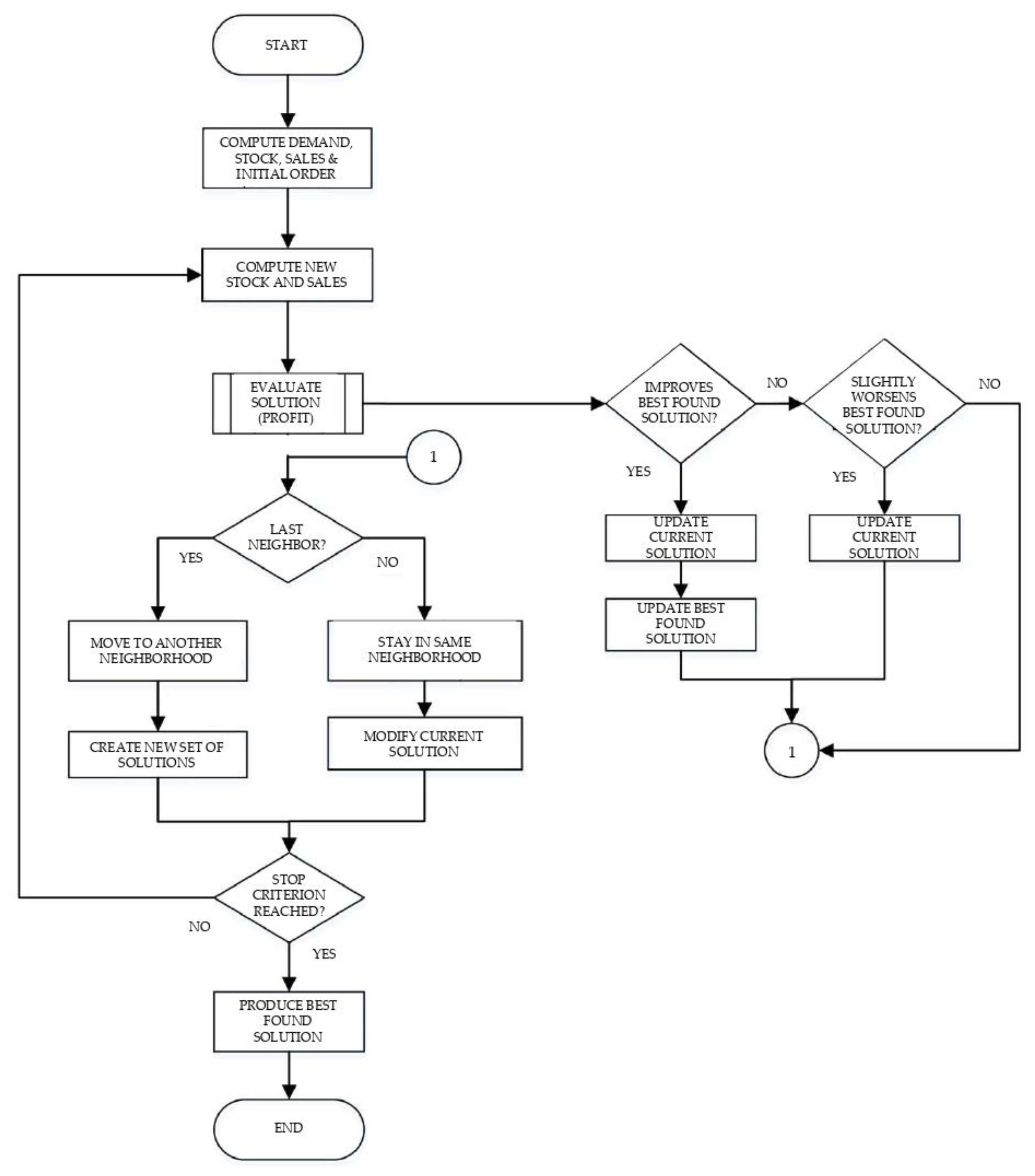
The characteristics of this problem entail that it presents an enormous number of feasible combinations. Therefore, the methodology employed seeks the best solution until a stopping criterion is met. Therefore, it cannot be guaranteed to be the optimal solution to the problem, but it is the best solution found so far (sub-optimal). The flowchart of the meta-heuristic is shown in
Figure 1 for guidance.
The flow chart is now briefly discussed to allow a better understanding of the methodology applied in solving the optimization problem.
Initially, starting from the sales forecast, a random demand is calculated within the range defined by Equation (3). A random order is determined as the current solution, and Equations (2) and (4) define the sales and inventory, respectively, for the first solution. This first solution will serve as a starting point to create a set of solutions (neighborhood: set of neighbors). All neighbors in a neighborhood are constructed from percentage variations of the order values. Such variation can be incremental or decremental within a range of 0 to 40%. It must be noted that a solution consists of the inventory of each type of product allocated to each channel in each of the periods considered.
Subsequently, a solution is evaluated from this set of solutions, and by doing so a profit is obtained, with three possibilities:
If the profit obtained is higher than the best profit found so far: the current solution is updated and this is taken as the best profit.
If the profit obtained is slightly lower than the best profit found so far: a random value will be generated to decide whether or not to update the current solution.
If the profit obtained is far from the best profit: Do nothing.
Once this solution was analyzed, we continued with the other solutions of the set (neighbors of the neighborhood). If it was the last solution, it went to a new neighborhood to create a new set of solutions. For this purpose, a new solution was generated, which was composed of a weighted average of three terms: the best solution found so far, the current solution and a random solution. The aim with this is to find solutions far removed from the ones that have already been evaluated but with the inheritance or influence of the best and current solutions. This solution generation fulfils the following relationship (the weights used were fixed after trial-and-error iterations):
A new solution was also tested by constructing a new solution from the arithmetic mean of the three terms mentioned above; however, this solution showed worse results, and the weighted average option was preferred. The expression would be:
Finally, the algorithm will only stop when the set stop condition is met, which can be an elapsed time limit for the simulation or a maximum number of iterations. Once one of these conditions has been met, the best results obtained so far will be displayed.
6. Results and Discussion
All the results achieved were possible thanks to a correct adjustment of the search parameters and the number of iterations to be carried out, in addition to other parameters that were correctly tuned by means of successive simulations. The results obtained from the example are shown below.
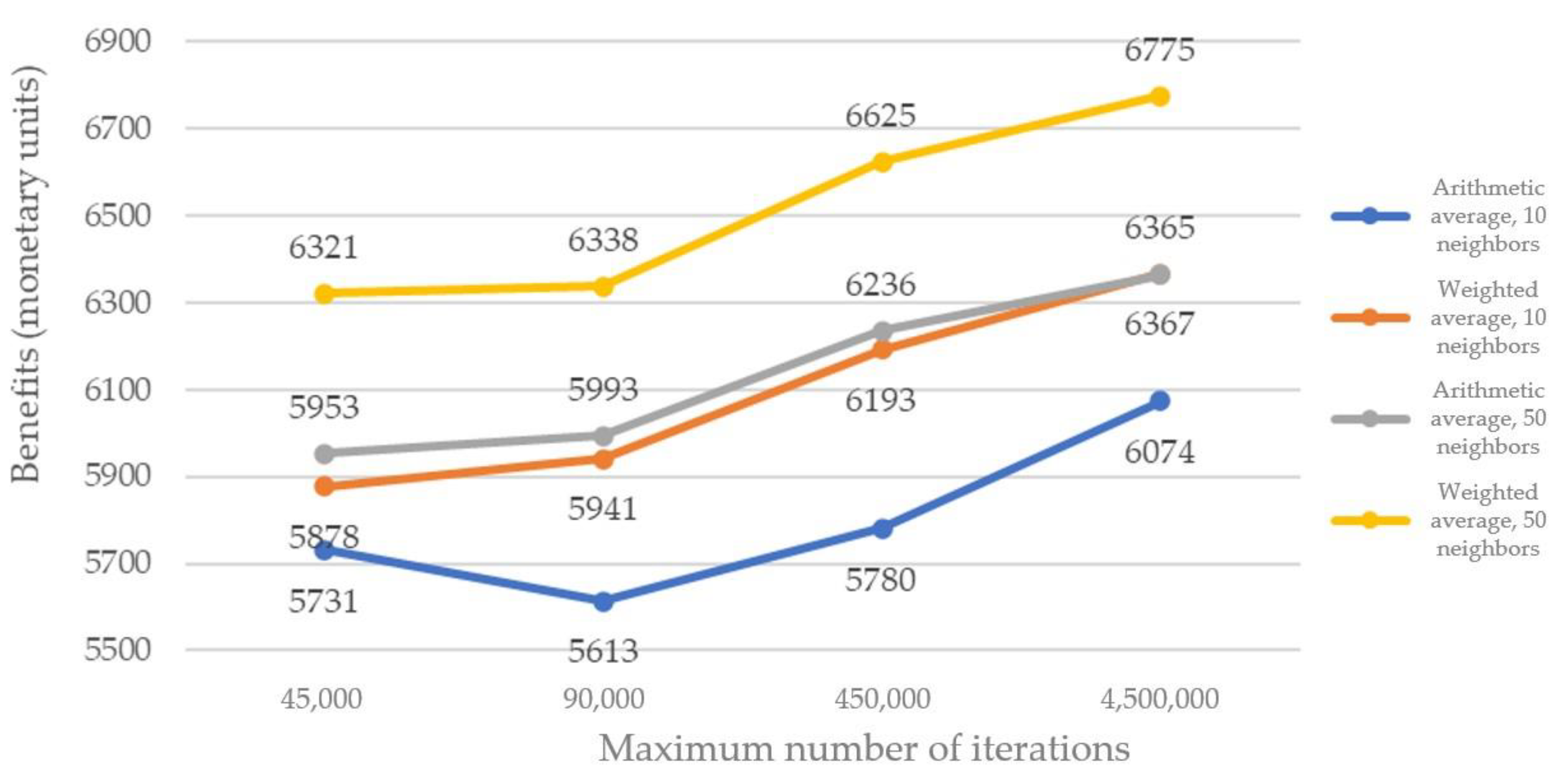
The differences in the profits obtained using the following methods are compared:
Mode of generating new solution sets: arithmetic or weighted average.
Local search mode: intensifying local search with larger neighborhoods (50 neighbors) and thus higher numbers of iterations, or prioritizing a more delocalized search with smaller neighborhoods (10 neighbors) and thus a lower number of iterations.
As can be seen in
Figure 2, we always obtained better solutions with the weighted average than with the arithmetic average (Equations (10) and (11), respectively), for both neighborhoods of 10 and 50 neighbors. Therefore, it is evident that when the generation of a new set of solutions has a strong influence on the best solution found so far (weighted average), a higher profit is achieved. On the other hand, this profit is smaller when the solution generated has a greater dependence on randomness (arithmetic mean). The positive point of randomness is that it allows a larger number of different neighborhoods to be tracked.
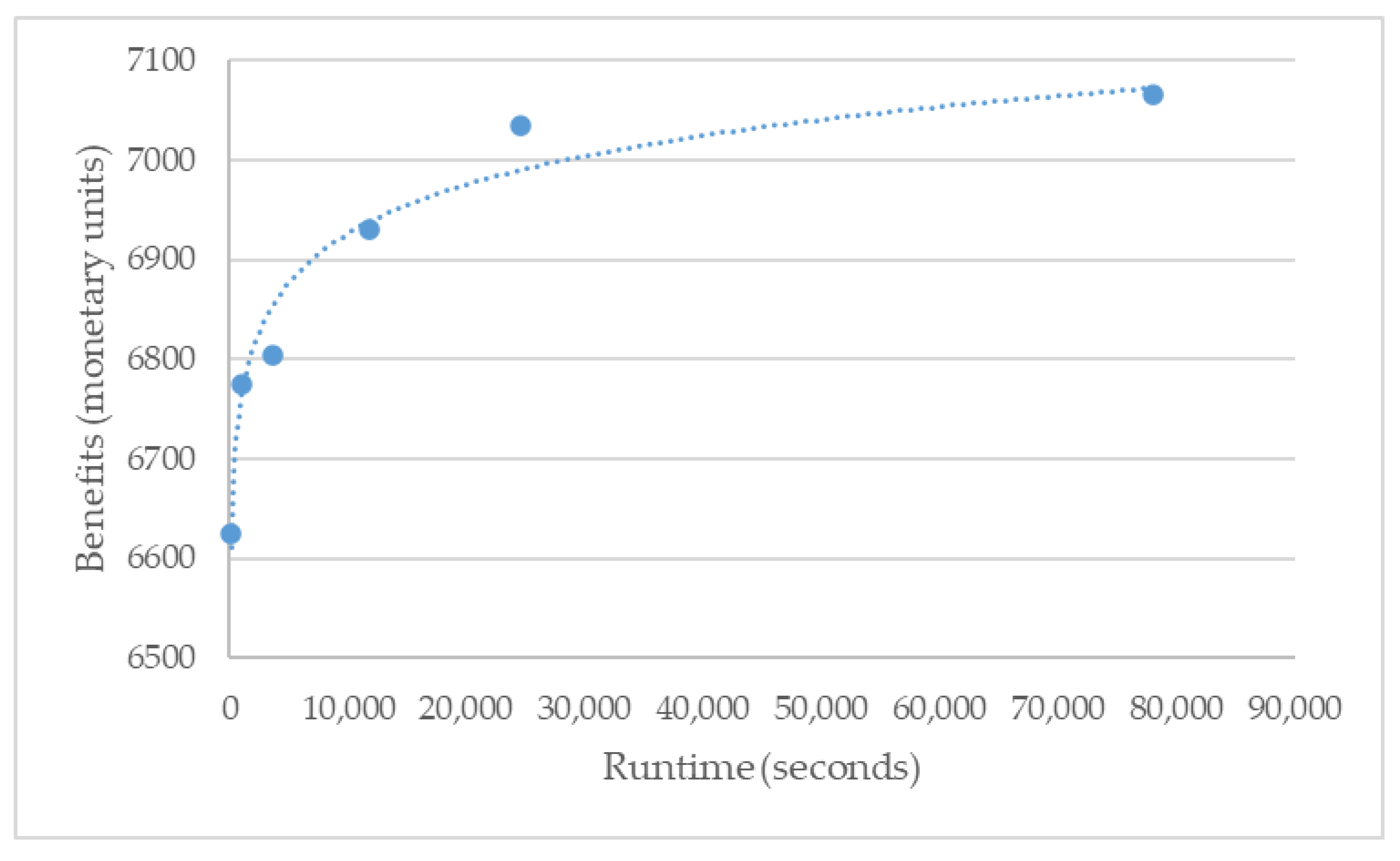
Once it has been proven that the best option is to generate a solution using the weighted average and for a neighborhood size of 50 individuals, it is necessary to evaluate how the profit would improve with respect to the program execution time. The longer the simulation time, the more solutions are sought and the more likely a better result is to be found. As seen in
Figure 3, it was decided to use run times from a couple of minutes to almost 22 h of simulation. The curve starts to flatten out for higher run times.
Figure 3 indicates that the benefits do improve with time but tend to stabilize after several hours of runtime, following a logarithmic pattern. The dotted line included in the graph represents a logarithmic trendline, which closely adheres to the evolution of the benefits. All the cases studied for different parameter values were repeated up to five times in order to take an average value, and thus obtain a more representative result.
To obtain these results, the metaheuristic was implemented in Python version 3.6.4 within the PyCharm 2017.3 environment, installed on a fixed computer with the following characteristics: Intel(R) Core™ i3-10100 3.6 GHz CPU, four main processors and 8.00 GB RAM.
The favorable evolution of the results and the significant improvements achieved in relatively short runtimes answer the research question proposed in this study positively. The results also indicate that this approach could be utilized in a dynamic manner, that is, being frequently rerun to replan for changes in demand or costs, amongst other model inputs, given the vast improvement to the objective function in a matter of 5 to 6 h of runtime. Furthermore, as expected, the results are very dependent on the parametrization of the metaheuristics [
46]. In this case, as seen in
Figure 2, the experimentation with the parameters affecting the mechanism for generating new solutions and the local search modes proves that superior solutions can be achieved if a weighted average generation mode with fifty solutions per neighborhood is used. However, the higher cost-efficiency of this parameter set for this particular instance of the problem does not guarantee that such combination would still be dominant in other applications. Thus, while the use of metaheuristic methods (in this case, a hybrid of the PSO and SA metaheuristics) proved useful for the efficient production of feasible solutions for the proposed depreciable-multiproduct omnichannel inventory replenishment problem, the results show that an exhaustive parametrization process must be conducted in order to fully optimize the method’s capabilities.
The use of metaheuristics (in this case, a hybrid of metaheuristics) allows the production of feasible and efficient solutions in short runtimes in comparison to other methods, such as mathematical programming, particularly when the problem scales up in size. Besides, a metaheuristic approach eases the translation of the method to other problems with expectedly similar results. Furthermore, even though the implementation of the metaheuristic itself addresses a particular set of constraints and a particular objective function, its structure and functioning are applicable to different fields of research.
7. Conclusions
In this work, we presented a hybrid-metaheuristic-based approach for the omnichannel, multiproduct inventory replenishment problem considering stock depreciation with time. The example problem, characteristic of a common retailer in the fashion sector, was solved in very limited runtimes, obtaining suboptimal solutions. The proposed metaheuristic combines elements of the PSO and SA algorithms. New solutions are obtained using the PSO neighborhood generation, and the movement to worse solutions in order to further explore the solution space is modelled using the SA logic.
Through the proposed approach, suboptimal solutions were achieved in short runtimes. In fact, the method could be incorporated as a real-time replenishment system, perhaps based on recalculating the inventory allocation using live demand data. This, of course, will only be applicable if real-time data of each channels’ demand can be obtained, and if the replenishment lead times are short enough to ensure that stock-outs do not occur in the meantime. If a live replenishment strategy were effectively implemented, the inventory levels at the shops and intermediate warehouses could be drastically reduced.
The metaheuristic proposed in this study is suitable for both multichannel and omnichannel environments. The methodology allows for the replenishment of several inventories, corresponding to either shops or intermediate warehouses. However, the dynamics of the sales and fulfillment processes are not addressed, and thus can be adapted to fit either an omnichannel or a multichannel paradigm.
The results of this study confirm the critical nature of efficient last-mile delivery management, particularly for fashion retailers. The expansion of the “free-shipping” strategy, the reduced profit margins and the growing complexity of freight distribution only foster the need for further research on the optimization of replenishment and distribution strategies. The cost reduction obtained by carefully balancing stock-out risk, product depreciation, sales fulfillment and transport costs is noteworthy, judging from the results shown in the study.
A limitation of this study was the deterministic character assumed for certain parameters of the model. Given the stochastic nature of demand, unit purchase cost and retail price, and their significant impacts on the operation of a replenishment network, including probability-based scenarios in the model and methodology could further increase the applicability of the presented approach to real-world settings.
A further line of research would be to adapt the proposed metaheuristic to replenishment problems, allowing the transhipment of stock between different channel locations. Additionally, the method could be adapted to perishable products, such as food, or even medical products, by strengthening the constraints on the delivery lead times of these products. Finally, in line with the growing interest in the use of machine learning and artificial intelligence techniques in the field of supply chain management, the optimization metaheuristic presented in this paper could be integrated with prediction models based on machine learning or neural network techniques, either for the optimization of the performance of the algorithm or for the forecasting of the model inputs.


