A Novel Approach to Extracting Casing Status Features Using Data Mining

Abstract

Casing coupling location signals provided by the magnetic localizer in retractors are typically used to ascertain the position of casing couplings in horizontal wells. However, the casing coupling location signal is usually submerged in noise, which will result in the failure of casing coupling detection under the harsh logging environment conditions. The limitation of Shannon wavelet time entropy, in the feature extraction of casing status, is presented by analyzing its application mechanism, and a corresponding improved algorithm is subsequently proposed. On the basis of wavelet transform, two derivative algorithms, singular values decomposition and Tsallis entropy theory, are proposed and their physics meanings are researched. Meanwhile, a novel data mining approach to extract casing status features with Tsallis wavelet singularity entropy is put forward in this paper. The theoretical analysis and experiment results indicate that the proposed approach can not only extract the casing coupling features accurately, but also identify the characteristics of perforation and local corrosion in casings. The innovation of the paper is in the use of simple wavelet entropy algorithms to extract the complex nonlinear logging signal features of a horizontal well tractor.

1. Introduction

In horizontal well production logging, it is necessary to detect casing status, including the position of casing couplings, perforations and any local corrosion [1–3]. The acquisition of accurate casing status information is significant for safe production and prognostication of the casing service life [4]. During horizontal well production logging, the retractor is an essential device to transport the logging instruments to testing points through horizontal well casings. To ascertain the creep speed and the position of the retractor in a horizontal well, a magnetic localizer in the retractor transmits casing coupling location (CCL) signals to data terminal equipment. According to the W-characteristic waveforms in the CCL signal, the operator can figure out the speed and position of the retractor in oil well casings. However, some negative impacts, such as multiphase flow and hidden flaws in well casings [5–7], can cause a decrease in the SNR of CCL signals, which may even result in the failure of casing coupling detection. If we could develop a novel data mining method to analyze CCL signals with low SNR further, the casing status feature information, including casing couplings, perforations, and local corrosion could be extracted, the logging procedure could be simplified, the logging efficiency increased, and the logging costs could be reduced.

In recent years, wavelet entropy is receiving growing attention for analyzing nonlinear signals [8,9]. As a novel data mining approach, wavelet entropy algorithm is employed to perform entropy operations on wavelet coefficients (or reconstruction signals) under various wavelet scales on the basis of wavelet transform and entropy theory. The main advantage of wavelet entropy is that it can realize the time-frequency localization of wavelet transforms and complexity estimation of entropy on nonlinear signals. Because wavelet entropy inherits the advantages of multi-scale wavelet transform and entropy, it has been applied in biological medicine, machinery, power system fault diagnosis and so on [10–16]. As a derivative approach of wavelet entropy, Shannon wavelet time entropy (WTE) has been used to analyze nonlinear signals. The Shannon WTE algorithm was introduced in detail and applied to diagnose transient faults in power systems, when power system transient disturbances including capacitor switching, lightning strikes and load start-stop occur, the features of transient signals can be extracted by analyzing the voltages and currents in the power grid by using Shannon WTE [12,13]. After discerning the similarities or differences among transient features, the transient disturbances can be classified into several categories and finally be verified with various classification methods. However, feature extraction based on Shannon WTE is not so effective, especially for original signals with low SNR, because the data dispersion partition is not reasonable. At the same time, Shannon entropy, as one portion of the Shannon WTE algorithm, is not adapted to evaluate the complexity of nonextensive systems.

In this paper, after analyzing the limitations of Shannon WTE used in casing status feature extraction, a novel data mining approach based on Tsallis wavelet singularity entropy (WSE) is proposed, and the physics meaning of the WSE derivative algorithms is researched. With the approach, the features of coupling, perforation, and local corrosion are extracted from CCL signals with noise and analyzed. Finally the results of our experimental research have been shown and are discussed.

2. Working Principle of Magnetic Localizer in Retractor and CCL Signal

To ascertain the speed and position of retractors creeping in horizontal well casings, a magnetic localizer including two Nd-Fe-B permanent magnets and a multi-turn induction coil are fixed in the retractor to supply the induced voltage of the CCL signal for the data acquisition module. In this paper, a 5000-turns induction coil is mounted between two magnets, its diameter and length are respectively 25.4 mm and 50.8 mm (Figure 1). A TMS320LF2812 DSP with a high-speed 12-bit ADC module, the key chip of the data acquisition module, is used to convert the induced voltage of the CCL signal into digital information and transmit it to data terminal equipment.

When the magnetic localizer passes by casing couplings, the magnetic flux changes immediately, which induces a fluctuation in the inductive-electromotive force in the induction coils (Figure 2), that indicates the number of casing couplings and provides original data for the calculation of the speed and position of the retractor.

Under realistic logging conditions, the SNR of CCL signals is very low, because there are a mass of noises caused by negative factors such as oil corrosion, multiphase flow, the compositional variety of the rock stratum and hidden flaws in well casings. Therefore the casing status feature information is sometimes submerged in noise and cannot be resolved directly as in Figure 3. We attempt to decompose the CCL signal into various scales using db4 wavelets in order to eliminate the high frequency interference and extract the casing coupling features, but the experimental results are still not desirable, which is analyzed in detail in Section 5. In order to solve this problem, Tsallis singularity entropy is proposed and applied to extract the casing status features from CCL signals with low SNR.

3. Disadvantage of Shannon WTE

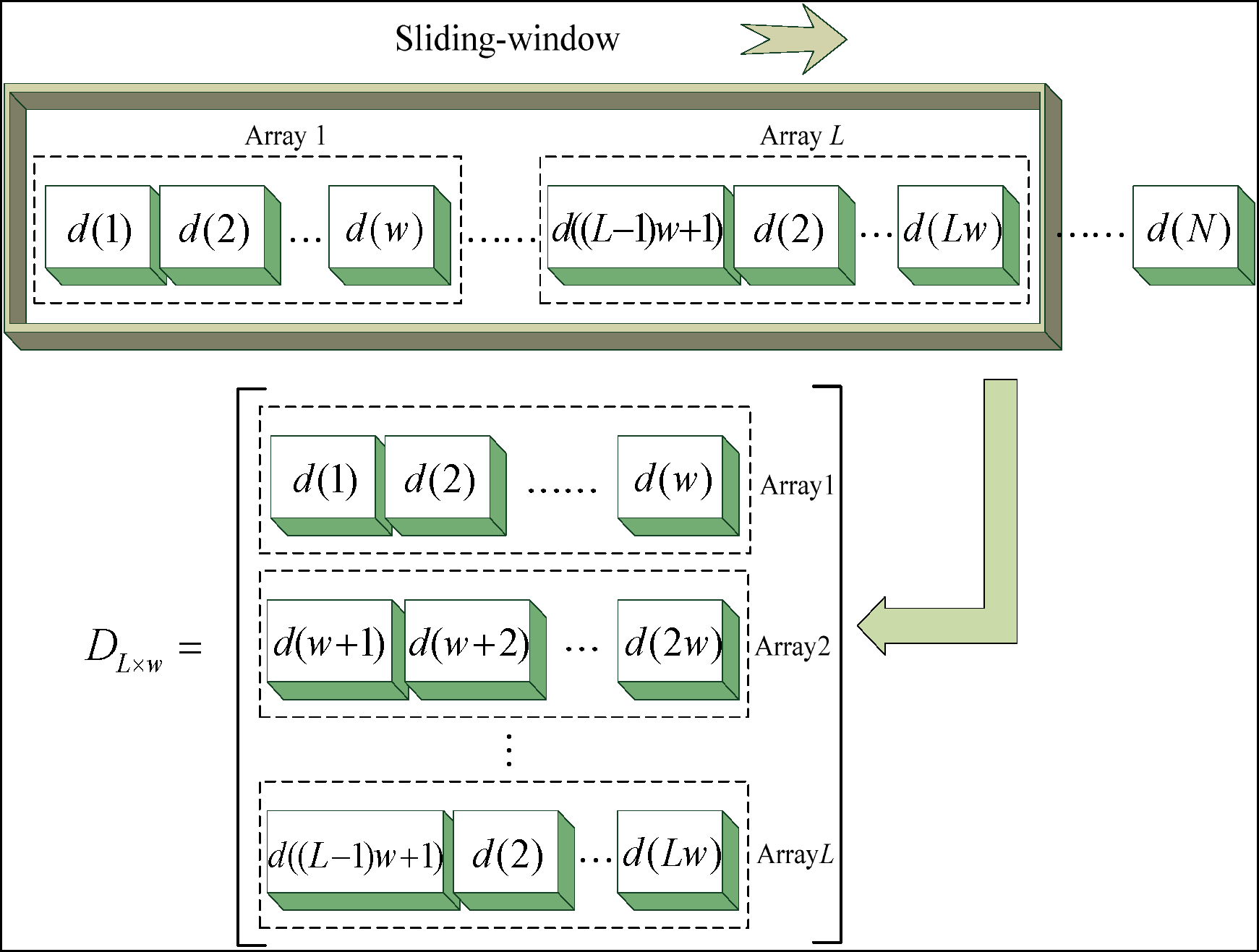
According to Shannon WTE definition [11,12], divided the sliding-window under wavelet coefficients (or reconstruction signals) into the following L segments $(W(m,w,\delta )=\underset{l=1}{\overset{L}{\cup }}{Z}_l)$, therein {Z_l = [s_l−1,s_l],l = 1,2,...,L} do not intersect. Moreover, s₀ < s₁ < ... < s_L, s₀ = min[W (m;w,δ)], and s_L = max[W(m;w,δ)]. Suppose that Sum_l is the amount of wavelet coefficients (or reconstruction signals) in Z_l, we obtain:

$$p^m(Z_l)=\frac{{\mathit{Sum}}_l}{w}$$

(1)

Therefore Shannon WTE under j scale is defined as follows:

$${\text{W}}_{\mathit{TE}}^j(m)=-\sum p^m(Z_l)\text{log}(p^m(Z_l))$$

(2)

where w is the width of the sliding-window, m = 1,2,...,M and M = (N−w)/δ ∈ N.

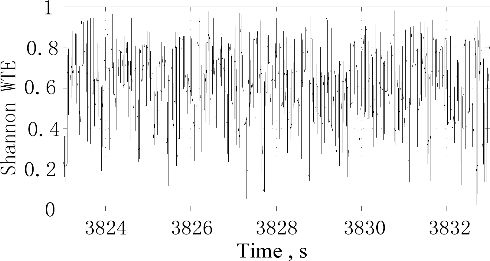
After CCL signal in Figure 3 is transformed on the db4 wavelet basis, when w = 100 and δ = 1, the Shannon WTE of A3 (approximate reconstruction signal under third scale) is obtained like Figure 4. According to Equations (1) and (2) from Figure 4, it is found that the casing coupling features are not extracted, despite the use of the Shannon WTE for A3.

Through the statistical calculation of data-dispersion density of Z_l in the sliding-window, about 70 percent of the total data exist from Z₆ to Z₁₅ in the approximate density, therefore:

$$p^m(Z_{\text{a}})\approx \frac{1}{10w}\sum _{a=6}^{15}{\mathit{Sum}}_a$$

(3)

where Sum_a is the amount of reconstruction signals in Z_a. The other scatter is in the different densities from Z₃ to Z₅ and from Z₁₆ to Z₁₈ .While the tractor is passing through casing couplings, about 5∼7 percent of the total data appear in Z₁, Z₂, Z₁₉, and Z₂₀. According to Equation (1), we can obtain:

$$\prod _{aequals;6}^{15}{\left(p^m\left(Z_a\right)\right)}^{-p^m\left(Z_a\right)}>(\prod _{bequals;3}^5{\left(p^m\left(Z_b\right)\right)}^{-p^m\left(Z_b\right)}+\prod _{cequals;16}^{18}{\left(p^m\left(Z_c\right)\right)}^{-p^m\left(Z_c\right)})\gg \prod _{dequals;1}^2{\left(p^m\left(Z_d\right)\right)}^{-p^m\left(Z_d\right)}+\prod _{\text{e}equals;19}^{20}{\left(p^m\left(Z_e\right)\right)}^{-p^m\left(Z_e\right)}$$

(4)

From Equations (2)–(4), we have:

$$\begin{array}{l}{\text{W}}_{\mathit{TE}}^j(m)=\text{ln}(\prod _{l=1}^{20}{(p^m(Z_l))}^{-p^m(Z_l)})\\ \hspace{0.17em}\hspace{0.17em}\hspace{0.17em}\hspace{0.17em}\hspace{0.17em}\hspace{0.17em}\hspace{0.17em}\hspace{0.17em}\hspace{0.17em}\hspace{0.17em}\hspace{0.17em}\hspace{0.17em}=\text{ln}(\prod _{\text{a}=6}^{15}{(p^m(Z_a))}^{-p^m(Z_a)})+\text{ln}(\prod _{\text{b}=3}^5{(p^m(Z_b))}^{-p^{m(Z_b)}})+\text{ln}\prod _{\text{c}=16}^{18}{(p^m(Z_c))}^{-p^{m(Z_c)}})\\ \hspace{0.17em}\hspace{0.17em}\hspace{0.17em}\hspace{0.17em}\hspace{0.17em}\hspace{0.17em}\hspace{0.17em}\hspace{0.17em}\hspace{0.17em}\hspace{0.17em}\hspace{0.17em}\hspace{0.17em}\hspace{0.17em}\hspace{0.17em}+\text{ln}(\prod _{\text{d}=1}^2{(p^m(Z_d))}^{-p^{m(Z_d)}})+\prod _{\text{e}=19}^{20}{(p^m(Z_e))}^{-p^{m(Z_e)}}\\ \hspace{0.17em}\hspace{0.17em}\hspace{0.17em}\hspace{0.17em}\hspace{0.17em}\hspace{0.17em}\hspace{0.17em}\hspace{0.17em}\hspace{0.17em}\hspace{0.17em}\hspace{0.17em}\hspace{0.17em}\hspace{0.17em}\hspace{0.17em}\hspace{0.17em}\hspace{0.17em}\approx \text{ln}(\prod _{l=3}^{18}(p^m{(Z_l))}^{-p^{m(Z_l)}})\end{array}$$

(5)

From Equation (5), we can know that the information feature is not extracted by using Shannon WTE as the most of data exist in the most fixed ranges while a few data corresponding to information features scatter in different densities in the special ranges. In view of the abovementioned facts, we make the following proposals to improve Shannon WTE algorithm. According to the data-dispersion density of the total range, the data range is divided into several asymmetric segments. The data range where there exists a large of noise information is roughly separated, while the data range where there exists little feature information is divided in a meticulous way. With the aid of this, the feature discernment will be promoted to a certain extent. However, the computational complexity is increased sharply with the improvement of the Shannon WTE algorithm.

4. The Tsallis Entropy and Wavelet Singularity Entropy

4.1. Tsallis Entropy

Tsallis entropy put forward by Tsallis in 1988, as nonextensive entropy, is the extension and deploitation of the extensive entropy (B-G entropy) in statistical physics [17]. It can explain some abnormal experiment phenomena, such as the complexity of non-additive systems, which cannot be explained by the theory of extensive entropy. Tsallis entropy in a discrete expression is defined as follows:

$${\text{S}}_q=\frac{\text{k}}{q-1}(1-\sum _{i=1}^{n}p{(i)}^q)\hspace{0.17em}(q\in R)$$

(6)

where k is Boltzmann constant, ${\{p(i)\}}_{i=1}^n$ is a probability distribution with i and $\sum _{i=1}^{n}p(i)=1$.

Different from extensive entropy, q is introduced as a parameter, so it is called nonextension index, and it represents the extent of nonextension of the system in Tsallis entropy. The nonadditivity of Tsallis entropy of a nonextensive system, composed of A and B subsystems, is defined as follows:

$$\frac{{\text{S}}_q(A+B)}{\text{k}}=\frac{{\text{S}}_q(A)}{\text{k}}+\frac{{\text{S}}_q(B)}{\text{k}}+(1-q)\frac{{\text{S}}_q(A){\text{S}}_q(B)}{{\text{k}}^2}$$

(7)

Note that q < 1 and q > 1 correspond respectively to the ultra-extensity and sub-extensity of the system. For researching the mathematical concave and convex nature of Tsallis entropy, let P and Q be probability variables, and satisfy P=(p(1),p(2),...,p(r)) and Q=(q(1),q(2),...,q(r)), where 0 ≤ p(i) ≤1, 0≤ q(i)≤1, i= 1,2,...r, $\sum _{i=1}^{r}p(i)=1$, and $\sum _{i=1}^{r}q(i)=1$. Suppose that 0 ≤ α ≤, when S_q satisfies:

$${\text{S}}_q(\alpha P+(1-\alpha )Q)\ge \alpha {\text{S}}_q(P)+(1-\alpha ){\text{S}}_q(Q)$$

(8)

The Tsallis entropy function represents the concave nature. At the same time, Tsallis entropy function has a definite concavity for all q values (S_q is concave for q > 0 and convex for q < 0). Furthermore, we consider Tsallis entropy statistical characteristics as two independent subsystems. According to Equation (6), we have a curves trace like Figure 5 which indicates the change law of Tsallis entropy with the probability distribution under different q values.

From Figure 5, the variation of q value has considerable effects on the statistical characteristics of Tsallis entropy. When q > 0 and q ≠ 1, the function curves take on the appearance of concavity, and there exists corresponding maximum values for all. When q → 1, Tsallis entropy is equivalent to B-G entropy and it can describe the complexity of an extensive system [18,19]. Moreover, when q < 0, the function curves are contrary to the former for q > 0, and there exists the corresponding minimum values. Based on the above analysis, Tsallis entropy with appropriate q value is not only more flexible in information measurement but more widespread in the statistical range of entropy.

4.2. Tsallis Wavelet Singularity Entropy

Let the wavelet coefficients (or reconstruction signals) of tested signal form D_{L × w} matrix, according to singular values decomposition principle, D_{L × w} is decomposed to:

$${\mathbf{D}}_{L\times w}={\mathbf{U}}_{L\times l}{\Lambda }_{l\times l}{\mathbf{V}}_{l\times w}$$

(9)

where D_{L × w} is L × w matrix, U_{L × l} is L × l matrix, V_{l × w} is l × w matrix and Λ_{l × l} is l × l diagonal singular matrix. Let the elements of the principal diagonal of Λ_{l × l} be λ_i(i= 1,2,...,l) and λ₁ ≥ λ₂ ≥ ... ≥ λ_l ≥ 0. At (m + w/2) moment, the discrete expression of Tsallis WSE is

$${\text{S}}_q(m)=\frac{\text{k}}{q-1}(1-\sum _{i=1}^n{p}_m{(i)}^q)$$

(10)

where $p_m(i)=\raisebox{1ex}{${\lambda }_i$}\!\left/ \!\raisebox{-1ex}{$\sum _{j=1}^l{\lambda }_j$}\right.$ According to the different elements chosen in D_{L × w}, two applications of the algorithm are presented as follows:

No. 1. Let A = {d(k), k= 1,2,...,N} be single wavelet coefficients (or reconstruction signals) under one wavelet scale, to form D_{L × w} (shown as Figure 6) at a length of w in the sliding-window. According to Equations (9) and (10), the No. 1 Tsallis WSE algorithm is obtained. The physical meaning of the No. 1 Tsallis WSE is analyzed as follows:

According to singular values decomposition theory and the definition of No. 1 Tsallis WSE, we find that the similarity among {d₁},{d₂},...{d_L} in the sliding-window is inversely proportional to the amount of λ_i(i= 1,2,...,l). When no feature information appears during this period of time, the similarity degree is to increase and the amount of λ_i not equal zero is to decrease contrarily, which results in the decline in the No. 1 Tsallis WSE value. On the contrary, when some feature information exists in the sliding-window, the similarity decreases and the amount of λ_i increases contrarily, which results in an increase of the No. 1 Tsallis WSE value.

No. 2. Let B = {d(g,k), g = 1,2,...,L,k= 1,2,…,N} be wavelet coefficients (or reconstruction signals) under L wavelet scales, a L × w sliding-window is built on B, and d(g, k) of B in the sliding-window form D_{L × w} (shown as Figure 7).

According to Equations (9) and (10), the No. 2 Tsallis WSE algorithm is obtained. The physical meaning of No. 2 Tsallis WSE is analyzed as follows:

According to the wavelet transform principle and relative knowledge, the correlation between wavelet coefficients (or reconstruction signals) under the neighboring scales is directly proportional to the similarity in their information components. From Equation (9), the amount of non-zero λ_i is to decrease as wavelet coefficients (or reconstruction signals) are approximately in accordance with each other, which results in a decline in the No. 2 Tsallis WSE value. On the contrary, as wavelet coefficients (or reconstruction signals) are distinctly different from each other, the amount of λ_i increases sharply, which results in an increase of the No. 2 Tsallis WSE value and proves that the amount of λ_i varies directly with the signal complexity. By using the No. 2 Tsallis WSE, the law of the change of signal complexity is described in detail.

From the above analysis, it can be concluded that the physical meaning of the Tsallis WSE is clear, and its algorithm is flexible and concise to meet the requirement of application, therefore, Tsallis WSE is applied to extract the features of coupling, perforation, and local corrosion from CCL signals with low SNR in this paper.

5. The Experimental Results

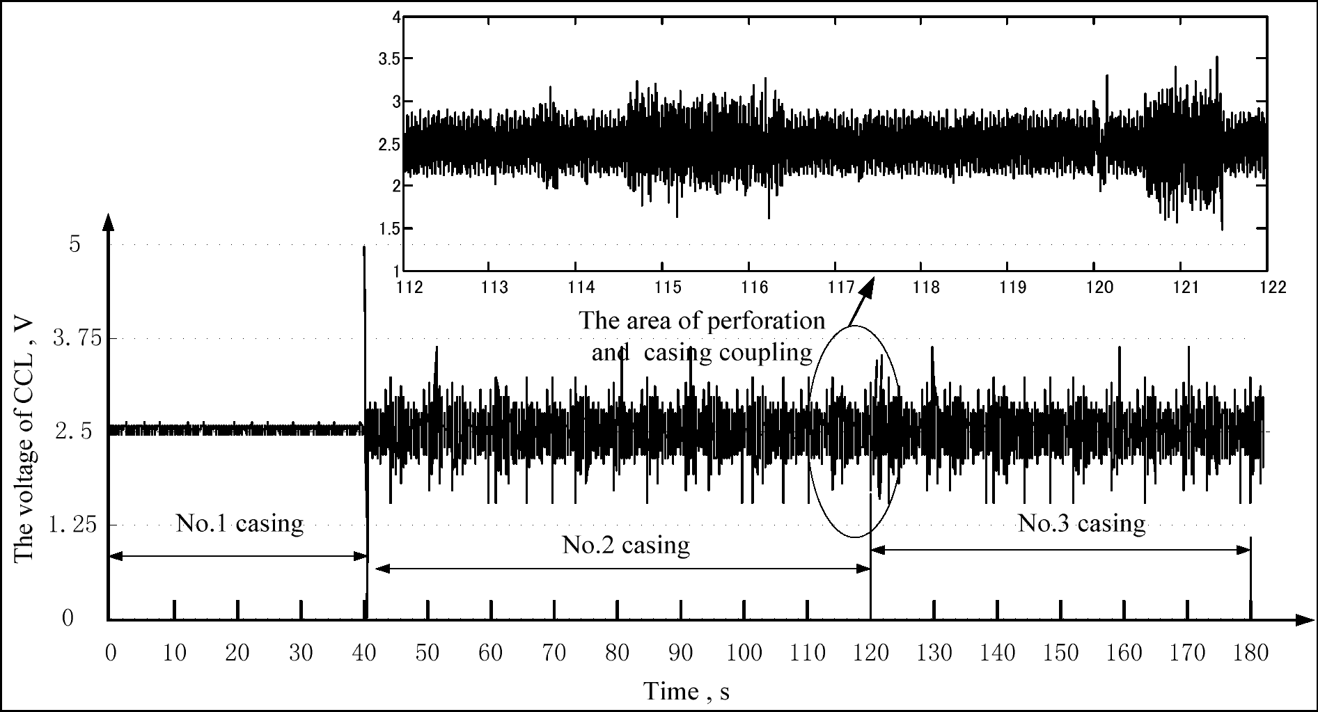
We establishs a testing platform, where three casings are connected together through casing couplings, to simulate the status of horizontal well casings. When a retractor creeps in the three casings, a CCL signal is collected by the magnetic localizer and transmitted to the data terminal equipment. The creep speed of the retractor, the sampling frequency, and the total time of data acquisition are respectively fixed at 100 mm/s, 1024 Hz and 180 s, and the parameters of the three casings are shown in

Table 1. Parameters of casings on the testing platform.

Casing number	Corrosion extent	Casing Length [mm]	CasingDiameter [mm]	Perforation number	Perforation Diameter [mm]	Perforation Interval [mm]
No. 1	slight	8000	140	0	/	/
No. 2	serious	8000	140	6	7	100
No. 3	serious	8000	140	0	/	/

. The induction voltage of the CCL signal is presented in Figure 8.

As shown in Figure 8, the induction voltage of CCL signal is close to 2.5 v without fluctuation in the No. 1 casing, while an obvious impulse signal occurs corresponding to the casing coupling between No. 1 casing and No. 2 casing. We can also find that the consecutive fluctuation of the induction voltage of the CCL signal, which occurs from 40 s to 180 s when the retractor creeps into the No. 2 casing and No. 3 casing. Furthermore, the signal features, corresponding to the casing coupling and the perforations between the No. 2 casing and No. 3 casing, are submerged in the noise caused by the serious corrosion of the two casings.

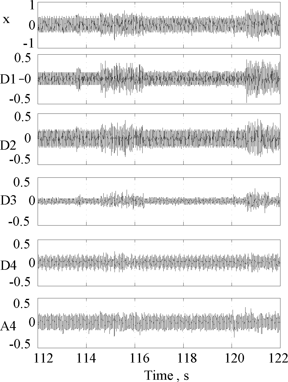
In the experiment, based on the retractor’s speed, the range of CCL signal frequencies corresponding to the casing couplings and the perforations is from 0.5 Hz to 2 Hz. If the sampling frequency is 1024 Hz and the normalized CCL signal is transformed to four scales by using the Mallat algorithm on db4, the casing coupling and perforation features in the CCL signal should exist in A4 (approximation reconstruction signal). However, during the time period of 112∼122 s, the features in A4 from Figure 9, corresponding to the casing coupling and perforations, are also submerged in the noise due to wavelet aliasing and noise in the same frequency band.

5.1. Feature Extraction Result with Shannon WTE

Through analyzing the mathematic structure of the Shannon WTE, we find that the relation between sliding-window width and transient signal duration is given as follows:

$$\{\begin{array}{ll}w=k\times T_{c\hspace{0.17em}\text{max}}\times f_s& (1<k\le 2)\\ 1\le \delta \le w& \end{array}$$

(11)

where T_c is transient signal duration.

In Equation (11), the reason why the range of w and δ are limited is to keep the feature information integrity and avoid the loss of key data in detected signals. Considering the retractor creep speed, the sampling frequency, the diameter of couplings and perforations, and the reasonable range of w and δ can be calculated out from Equation (11). Here, we set w = 120, δ = 1, and L = 20, where L is the segment number in the sliding-window.

Taking the approximation reconstruction signal A4 in Figure 9 as the analysis object, because there the casing coupling and perforations features exist in A4, we calculate the Shannon WTE of CCL according to Equations (1) and (2), and the normalized calculation results of the Shannon WTE are shown in Figure 10a.

From Figure 10a, although the Shannon WTE algorithm is used, the casing coupling and perforation features are still not extracted. Based on the improved Shannon WTE, the similar calculation process is done again, and the normalized calculation results of the improved Shannon WTE are shown in Figure 10b. Comparing Figure 10a with Figure 10b, it is found that a great improvement has been made in perforation feature extraction by the novel method, in comparison with the traditional way, as the improved Shannon entropy divides the data range into several asymmetric segments according to the data-dispersion density. However, the loss of features of perforation No. 2 and No. 3 still occurs in Figure 10b, and there is no obvious difference between coupling features and perforation features, which could result in feature recognition errors.

To explain the reason why the improved Shannon WTE failed to extract the features of the No. 2 and No. 3 perforation, we do the following: first of all, we get the A4 signal shown in Figure 9. Then, we calculate the data distribution statistics of the A4 signal, by utilizing the improved Shannon WTE which divides the data range into uneven segments. The statistics result is shown in Figure 11. The uneven data distribution is to merge subsegments 5 to 16, by the even data distribution method, into one subsegment, and divide the rest into 20 segments, according to the principle that the data range, where there exists larger data density, is separated roughly, while the data range, where there exist smaller data density, is divided in a meticulous way. From Figure 11, the data distribution range of No. 1, 4, 5 and 6 perforations is mainly in segments 1 to 10, however, the noise data is distributed in segments 11 to 13. On the basis of the related proofs of Equation (5), for perforation data (the data of a small probability event), the uneven data distribution will have a larger entropy than the even distribution method, but for the noise data, the opposite is true, which has been shown in Figure 10b. By utilizing the improved Shannon WTE, the mean value of the corresponding CCL signal of No. 5 perforation E_e = 1.4509, the mean value of the noise E_noise = 1.1463, the feature difference rate $\delta =\frac{\left|E_e-E_{\mathit{noise}}\right|}{E_{\mathit{noise}}}\times 100\%=27\%$. However, the No. 2 and No. 3 perforations have serious peripheral corrosion and their apertures become narrow, so the energy of the perforation feature signal is weak and submerged in noise. Meanwhile, there is no data in subsegments 1 to 7. Here the mean value of the improved Shannon WTE of No. 2 perforation E_e = 1.1123, and δ = 2.97%, the mean value of the improved Shannon WTE of No. 3 perforation E_e = 1.2391, and δ = 8.1%. The feature difference is not obvious, so it has failed to extract the features of these two perforations. Therefore, the improved Shannon WTE method still relies on data scatter statistics of subsegments and the Shannon entropy algorithm, which makes it hard to precisely extract features of those perforation signals with low SNR.

5.2. Feature Extraction Results with the No. 1 Tsallis WSE

Through researching Tsallis WSE in Section 4, it is found that the No. 1 algorithm of the Tsallis WSE is better suited for extracting low-energy featurees for signals with low SNR. In order to keep the integrity of feature information and reduce calculative complexity, the range of w and δ are defined as follows:

$$\{\begin{array}{ll}w=\frac{k\times T_{c\hspace{0.17em}\text{max}}\times f_s}{L}\hfill & (1<K<1.5)\hfill \\ 1\le \delta \le w\hfill & \hfill \end{array}$$

(12)

According to Equation (12), the value of w can be calculated as L = 4 and T_cmax ≈ 0.075 s. As w = 18, δ = 1 and L = 4, the casing coupling and perforation features are extracted from A4 with No. 1 Tsallis WSE, and the normalized calculation results are shown in Figure 12. Therein, six triangle-characteristic waveforms, which are 0.4∼0.5 pu high and 0.056∼0.090 s wide, appear to indicate the existence of six perforations when the magnetic localizer passes by the perforation zone in the No. 2 casing from 112 s to 119 s. A M-characteristic waveform, which is 0.6∼0.7 pu high and 1.1∼1.4 s wide, and which appears from 120.1 s to 121.4 s, reflects the existence of a casing coupling between the No. 2 casing and No. 3 casing. According to the above analysis, the physical distance and size of perforation can be calculated by observing the triangle-characteristic waveform, and the position and junction status of casing couplings also can be figured out by observing the M-characteristic waveform.

In order to further compare the difference between the improved Shannon WTE and Tsallis WSE in terms of feature extraction of the perforations, the magnetic localizer of the retractor is used to collect CCL signals of casings with perforations with different degrees of corrosion in Figure 13. In addition, we extract the perforation features of the collected CCL signals by using the two methods above. We randomly choose 60 perforation samples and 60 non-perforation samples as the testing sample from the feature extraction results. Because a complex process exists when extracting and recognizing casing features, we cannot adopt simple indicators. For instance, we take the peak feature or period width of a sample as the detection threshold. Since we have to start with all the perforation features and consider the macro and micro aspects, therefore, similarity of testing sample and standard sample of perforation feature is adopted as the optimal target, which not only accords with the custom of artificial cognition, but also overcomes the drawback of a single indicator. The similarity is taken as the threshold which varies from 100% to 60%, and then the parameters of TP and FP are separately counted as shown in

Table 2. Statistical results for feature extraction of perforations based on the two approaches.

Similarity [%]	Approach	Testing sample sum	TP	FP	FN	TN	ACC [%]
100	Improved Shannon WTE	120	0	0	60	60	0
	Tsallis WSE	120	0	0	60	60	0
95	Improved Shannon WTE	120	40	1	20	59	82.5
	Tsallis WSE	120	47	0	13	60	89.2
85	Improved Shannon WTE	120	43	3	17	57	83.3
	Tsallis WSE	120	52	1	8	59	92.5
75	Improved Shannon WTE	120	47	6	13	54	84.2
	Tsallis WSE	120	54	2	6	58	93.3
70	Improved Shannon WTE	120	50	10	10	50	83.3
	Tsallis WSE	120	56	3	4	57	94.2
60	Improved Shannon WTE	120	51	16	9	44	79.2
	Tsallis WSE	120	58	5	2	55	94.2

. By analyzing Table 2, for the improved Shannon WTE, the number of FP samples increases sharply as the similarity threshold constantly decreases. For instance, there is one FP sample with similarity = 95% while 16 FP samples have similarity = 60%, which represents a decline in the feature extraction accuracy. However, the FP sample amount of the Tsallis WSE has remained at low levels (5 samples with similarity = 60%), its feature extraction accuracy remains above 90% except for slight fluctuations. As a whole, Tsallis WSE is better than the former.

The ROC plot is used to reflect the difference between two methods in perforation feature extraction ability. We calculate the TPR and FPR of the two feature extraction methods and draw ROC plots as shown in Figure 14. According to this Figure, the growth rate of FPR of the improved Shannon WTE is much faster than Tsallis WSE with a falling similarity threshold in a range of 85%∼60%, which means that there exists inaccuracy in the perforation feature extraction, based on the improved Shannon WTE. When the similarity threshold falls, some non-perforations are mistaken for perforations, thus the accuracy decreases, as shown in Figure 10b. The above analysis shows that Tsallis WSE operates better than the improved Shannon WTE in perforation feature extraction. Meanwhile, it can be deduced that choosing a similarity threshold in a range of 70%∼85% is reasonable for classifying the results of perforation feature extraction with similarity theory. An inappropriate similarity threshold will have negative effect on the subsequent feature classification.

5.3. The Feature Extraction of Local Casing Corrosion with No. 2 Tsallis WSE

Under the condition of w = 350, L = 4 and δ = 1, taking D1∼D4 mentioned above as the analyzed signals, we extract casing local corrosion according to the definition of No. 2 Tsallis WSE and the its normalized curve is drawn as Figure 15. We can find that the magnitude of No. 2 Tsallis WSE is directly proportional to the complexity of the CCL signal, which reflects the extent of local corrosion in casings. During the three periods, 113.4 s to 113.8 s, 114.5 s to 116.3 s and 120.5 s to 122 s, three distinct peaks appear to indicate the local casing corrosion existing between No. 2 casing and No. 3 casing. From these evidences, the distributed location and the extent of local casing corrosion can be known by taking the speed of retractor into account.

6. Conclusions

For the above mentioned research and experiment evidence, the main conclusions are as follows:

(1)

Dividing the data dispersion range mechanically results in a declined sensitivity of the Shannon WTE to the feature information hidden in the original signals. When CCL signals under low SNR are taken as the analysis object, the casing status features cannot be extracted using the Shannon WTE algorithm. Although the capability to extract features is improved, the improved Shannon WTE algorithm still has some disadvantages in feature extraction in the strong noisy background.

(2)

Tsallis WSE, as the composition of wavelet transform, singular values decomposition and Tsallis entropy, inherits the advantages of wavelet transform and Tsallis entropy. The singular features of low SNR signals can be extracted using its derivate algorithm. As the complexity of Tsallis WSE algorithm and improved Shannon WTE are at the same level, the feature extraction effect of the Tsallis WSE algorithm is better than that of the improved Shannon WTE.

(3)

Using Tsallis WSE to complete data mining of CCL signals, we successfully extracted the feature information corresponding to casing couplings, perforations and extent of local corrosion. Consequently, the casing status detection process is simplified and can supply valid data for horizontal well production logging.

References

- Amro, M.M. Effect of scale and corrosion inhibitors on well productivity in reservoirs containing asphaltenes. J. Pet. Sci. Eng 2005, 46, 243–252. [Google Scholar]
- Thorsen, A.K.; Eiane, T.; Thern, H.F.; Fristad, P.; Williams, S. Magnetic resonance in chalk horizontal well logged with LWD. SPE Reserv. Eval. Eng 2010, 13, 654–666. [Google Scholar]
- Wang, Z.M.; Wei, J.G.; Jin, H. Partition perforation optimization for horizontal wells based on genetic algorithms. SPE Drill. Complet 2011, 26, 52–59. [Google Scholar]
- Tabatabaei, M.; Ghalambor, A. A. New Method to Predict Performance of Horizontal and Multilateral Wells. In Proceedings of the International Petroleum Technology Conference, Doha, Qatar, 7–9 December 2009.
- Gokcal, B.; Wang, Q.; Zhang, H.Q.; Sarica, C. Effects of high oil viscosity on oil/gas flow behavior in horizontal pipes. SPE Proj. Facil. Constr 2008, 3, 1–11. [Google Scholar]
- Li, S.X.; Yu, S.R.; Zeng, H.L.; Li, J.H.; Liang, R. Predicting corrosion remaining life of underground pipelines with a mechanically-based probabilistic model. J. Pet. Sci. Eng 2009, 65, 162–166. [Google Scholar]
- Gao, Z.K.; Jin, N.D.; Wang, W.X.; Lai, Y.C. Motif distributions in phase-space networks for characterizing experimental two-phase flow patterns with chaotic features. Phys. Rev. E 2010, 82, 016210. [Google Scholar]
- Richman, J.S.; Moorman, J.R. Physiological time-series analysis using approximate entropy and sample entropy. Am. J. Physiol. Heart Circ. Physiol 2000, 278, H2039–H2049. [Google Scholar]
- Yan, J.J.; Wang, Y.Q.; Guo, R.; Zhou, J.Z.; Yan, H.X.; Xia, C.M.; Shen, Y. Nonlinear analysis of auscultation signals in TCM using the combination of wavelet packet transform and sample entropy. Evid. Based Complement Alternat. Med 2012. [Google Scholar] [CrossRef]
- Al-Nashash, H.A.; Thakor, N.V. Monitoring of global cerebral ischemia using wavelet entropy rate of change. IEEE Trans. Biomed. Eng 2005, 52, 2119–2122. [Google Scholar]
- Feng, Z.Y.; Chen, H. Analyze the Dynamic Features of Rat EEG Using Wavelet Entropy. In Proceedings of the 2005 IEEE Engineering in Medicine and Biology 27th Annual Conference, Shanghai, China, 1–4 September 2005.
- He, Z.Y.; Cai, Y.M.; Qian, Q.Q. A study of wavelet entropy theory and its application in electric power system fault detection. Proc. Chin. Soc. Electr. Eng 2005, 25, 38–43. [Google Scholar]
- He, Z.Y.; Chen, X.Q.; Luo, G.M. Wavelet Entropy Measure Definition and Its Application for Transmission Line Fault Detection and Identification. In Proceedings of the International Conference on Power System Technology, Chongqing, China, 22–26 October 2006.
- Lemire, D.; Pharand, C.; Rajaonah, J.; Dubé, B.; LeBlanc, A.R. Wavelet time entropy, T wave morphology and myocardial ischemia. IEEE Trans. Biomed. Eng 2000, 47, 967–970. [Google Scholar]
- Cek, M.E.; Ozgoren, M.; Savaci, F.A. Continuous time wavelet entropy of auditory evoked potentials. Comput. Biol. Med 2010, 40, 90–96. [Google Scholar]
- Zhang, L.; He, C.H.; He, W. Characterization of Cerebral Infarction in Multiple Channel EEG Recordings Based on Quantifications of Time-Frequency Representation. In Proceedings of the International Conference on Life System Modeling and Simulation, Wuxi, China, 17–20 September 2010.
- Tsallis, C.; Mendes, R.S.; Plastino, A.R. The role of constraints within generalized nonextensive statistics. Physica A 1998, 261, 534–554. [Google Scholar]
- Martins, A.; Aguiar, P.; Figueiredo, M. Tsallis Kernels on Measures. In Proceedings of the IEEE Information Theory Workshop, Porto, Portugal, 5–9 May 2008.
- Sneddon, R. The Tsallis entropy of natural information. Physica A 2007, 386, 101–118. [Google Scholar]