
Tail Risk Constraints and Maximum Entropy

1
Department of Applied Mathematics & Statistics, Johns Hopkins University, Baltimore, MD 21218-2608, USA
2
Department of Economics, Mathematics and Statistics, Birkbeck, University of London, London WC1E 7HX, UK
3
Polytechnic School of Engineering, New York University, New York, NY 11201, USA
*
Author to whom correspondence should be addressed.
Entropy 2015, 17(6), 3724-3737; https://0-doi-org.brum.beds.ac.uk/10.3390/e17063724
Submission received: 3 March 2015
/
Revised: 15 May 2015
/
Accepted: 22 May 2015
/
Published: 5 June 2015
(This article belongs to the Special Issue Information Processing in Complex Systems)
Abstract
:Portfolio selection in the financial literature has essentially been analyzed under two central assumptions: full knowledge of the joint probability distribution of the returns of the securities that will comprise the target portfolio; and investors’ preferences are expressed through a utility function. In the real world, operators build portfolios under risk constraints which are expressed both by their clients and regulators and which bear on the maximal loss that may be generated over a given time period at a given confidence level (the so-called Value at Risk of the position). Interestingly, in the finance literature, a serious discussion of how much or little is known from a probabilistic standpoint about the multi-dimensional density of the assets’ returns seems to be of limited relevance. Our approach in contrast is to highlight these issues and then adopt throughout a framework of entropy maximization to represent the real world ignorance of the “true” probability distributions, both univariate and multivariate, of traded securities’ returns. In this setting, we identify the optimal portfolio under a number of downside risk constraints. Two interesting results are exhibited: (i) the left- tail constraints are sufficiently powerful to override all other considerations in the conventional theory; (ii) the “barbell portfolio” (maximal certainty/low risk in one set of holdings, maximal uncertainty in another), which is quite familiar to traders, naturally emerges in our construction.
1. Left Tail Risk as the Central Portfolio Constraint
Customarily, when working in an institutional framework, operators and risk takers principally use regulatorily mandated tail-loss limits to set risk levels in their portfolios (obligatorily for banks since Basel II). They rely on stress tests, stop-losses, value at risk (VaR), expected shortfall (i.e., the expected loss conditional on the loss exceeding VaR, also known as CVaR), and similar loss curtailment methods, rather than utility. In particular, the margining of financial transactions is calibrated by clearing firms and exchanges on tail losses, seen both probabilistically and through stress testing. (In the risk-taking terminology, a stop loss is a mandatory order that attempts terminates all or a portion of the exposure upon a trigger, a certain pre-defined nominal loss. Basel II is a generally used name for recommendations on banking laws and regulations issued by the Basel Committee on Banking Supervision. The Value-at-risk, VaR, is defined as a threshold loss value K such that the probability that the loss on the portfolio over the given time horizon exceeds this value is ϵ. A stress test is an examination of the performance upon an arbitrarily set deviation in the underlying variables.) The information embedded in the choice of the constraint is, to say the least, a meaningful statistic about the appetite for risk and the shape of the desired distribution.
Operators are less concerned with portfolio variations than with the drawdown they may face over a time window. Further, they are in ignorance of the joint probability distribution of the components in their portfolio (except for a vague notion of association and hedges), but can control losses organically with allocation methods based on maximum risk. (The idea of substituting variance for risk can appear very strange to practitioners of risk-taking. The aim by Modern Portfolio Theory at lowering variance is inconsistent with the preferences of a rational investor, regardless of his risk aversion, since it also minimizes the variability in the profit domain—except in the very narrow situation of certainty about the future mean return, and in the far-fetched case where the investor can only invest in variables having a symmetric probability distribution, and/or only have a symmetric payoff. Stop losses and tail risk controls violate such symmetry.) The conventional notions of utility and variance may be used, but not directly as information about them is embedded in the tail loss constaint.
Since the stop loss, the VaR (and expected shortfall) approaches and other risk-control methods concern only one segment of the distribution, the negative side of the loss domain, we can get a dual approach akin to a portfolio separation, or “barbell-style” construction, as the investor can have opposite stances on different parts of the return distribution. Our definition of barbell here is the mixing of two extreme properties in a portfolio such as a linear combination of maximal conservatism for a fraction w of the portfolio, with w ∈ (0, 1), on one hand and maximal (or high) risk on the (1−w) remaining fraction.
Historically, finance theory has had a preference for parametric, less robust, methods. The idea that a decision-maker has clear and error-free knowledge about the distribution of future payoffs has survived in spite of its lack of practical and theoretical validity—for instance, correlations are too unstable to yield precise measurements. It is an approach that is based on distributional and parametric certainties, one that may be useful for research but does not accommodate responsible risk taking. (Correlations are unstable in an unstable way, as joint returns for assets are not elliptical, see Bouchaud and Chicheportiche (2012) [1].)
There are roughly two traditions: one based on highly parametric decision-making by the economics establishment (largely represented by Markowitz [2]) and the other based on somewhat sparse assumptions and known as the Kelly criterion (Kelly, 1956 [3], see Bell and Cover, 1980 [4].) (In contrast to the minimum-variance approach, Kelly’s method, developed around the same period as Markowitz, requires no joint distribution or utility function. In practice one needs the ratio of expected profit to worst-case return dynamically adjusted to avoid ruin. Obviously, model error is of smaller consequence under the Kelly criterion: Thorp (1969) [5], Haigh (2000) [6], Mac Lean, Ziemba and Blazenko [7]. For a discussion of the differences between the two approaches, see Samuelson’s objection to the Kelly criterion and logarithmic sizing in Thorp 2010 [8].) Kelly’s method is also related to left- tail control due to proportional investment, which automatically reduces the portfolio in the event of losses; but the original method requires a hard, nonparametric worst-case scenario, that is, securities that have a lower bound in their variations, akin to a gamble in a casino, which is something that, in finance, can only be accomplished through binary options. The Kelly criterion, in addition, requires some precise knowledge of future returns such as the mean. Our approach goes beyond the latter method in accommodating more uncertainty about the returns, whereby an operator can only control his left-tail via derivatives and other forms of insurance or dynamic portfolio construction based on stop-losses. (Xu, Wu, Jiang, and Song (2014) [9] contrast mean variance to maximum entropy and uses entropy to construct robust portfolios.)
In a nutshell, we hardwire the curtailments on loss but otherwise assume maximal uncertainty about the returns. More precisely, we equate the return distribution with the maximum entropy extension of constraints expressed as statistical expectations on the left-tail behavior as well as on the expectation of the return or log-return in the non-danger zone. (Note that we use Shannon entropy throughout. There are other information measures, such as Tsallis entropy [10], a generalization of Shannon entropy, and Renyi entropy, [11], some of which may be more convenient computationally in special cases. However, Shannon entropy is the best known and has a well-developed maximization framework.)
Here, the “left-tail behavior” refers to the hard, explicit, institutional constraints discussed above. We describe the shape and investigate other properties of the resulting so-called maxent distribution. In addition to a mathematical result revealing the link between acceptable tail loss (VaR) and the expected return in the Gaussian mean-variance framework, our contribution is then twofold: (1) an investigation of the shape of the distribution of returns from portfolio construction under more natural constraints than those imposed in the mean-variance method, and (2) the use of stochastic entropy to represent residual uncertainty.
VaR and CVaR methods are not error free—parametric VaR is known to be ineffective as a risk control method on its own. However, these methods can be made robust using constructions that, upon paying an insurance price, no longer depend on parametric assumptions. This can be done using derivative contracts or by organic construction (clearly if someone has 80% of his portfolio in numéraire securities, the risk of losing more than 20% is zero independent from all possible models of returns, as the fluctuations in the numéraire are not considered risky). We use “pure robustness” or both VaR and zero shortfall via the “hard stop” or insurance, which is the special case in our paper of what we called earlier a “barbell” construction.
It is worth mentioning that it is an old idea in economics that an investor can build a portfolio based on two distinct risk categories, see Hicks (1939) [12]. Modern Portfolio Theory proposes the mutual fund theorem or “separation” theorem, namely that all investors can obtain their desired portfolio by mixing two mutual funds, one being the riskfree asset and one representing the optimal mean-variance portfolio that is tangent to their constraints; see Tobin (1958) [13], Markowitz (1959) [14], and the variations in Merton (1972) [15], Ross (1978) [16]. In our case a riskless asset is the part of the tail where risk is set to exactly zero. Note that the risky part of the portfolio needs to be minimum variance in traditional financial economics; for our method the exact opposite representation is taken for the risky one.
1.1. The Barbell as seen by E.T. Jaynes
Our approach to constrain only what can be constrained (in a robust manner) and to maximize entropy elsewhere echoes a remarkable insight by E.T. Jaynes in “How should we use entropy in economics?” [17]:
“It may be that a macroeconomic system does not move in response to (or at least not solely in response to) the forces that are supposed to exist in current theories; it may simply move in the direction of increasing entropy as constrained by the conservation laws imposed by Nature and Government.”
2. Revisiting the Mean Variance Setting
Let
denote m asset returns over a given single period with joint density
, mean returns
and m×m covariance matrix
, 1 ≤ i, j ≤ m. Assume that
and Σ can be reliably estimated from data.
The return on the portolio with weights
is then
which has mean and variance
In standard portfolio theory one minimizes V (X) over all
subject to
for a fixed desired average return μ. Equivalently, one maximizes the expected return
subject to a fixed variance V (X). In this framework variance is taken as a substitute for risk.
To draw connections with our entropy-centered approach, we consider two standard cases:
- Normal World: The joint distribution of asset returns is multivariate Gaussian . Assuming normality is equivalent to assuming has maximum (Shannon) entropy among all multivariate distributions with the given first- and second-order statistics and Σ. Moreover, for a fixed mean , minimizing the variance V (X) is equivalent to minimizing the entropy (uncertainty) of X. (This is true since joint normality implies that X is univariate normal for any choice of weights and the entropy of a N(μ, σ2) variable is .) This is natural in a world with complete information. (The idea of entropy as mean uncertainty is in Philippatos and Wilson (1972) [18]; see Zhou et al. (2013) [19] for a review of entropy in financial economics and Georgescu-Roegen (1971) [20] for economics in general.)
- Unknown Multivariate Distribution: Since we assume we can estimate the second-order structure, we can still carry out the Markowitz program, i.e., choose the portfolio weights to find an optimal mean-variance performance, which determines and V (X) = σ2. However, we do not know the distribution of the return X. Observe that assuming X is normal N(μ, σ2) is equivalent to assuming the entropy of X is maximized since, again, the normal maximizes entropy at a given mean and variance, see [18].
Our strategy is to generalize the second scenario by replacing the variance σ2 by two left-tail value-at-risk constraints and to model the portfolio return as the maximum entropy extension of these constraints together with a constraint on the overall performance or on the growth of the portfolio in the non-danger zone.
2.1. Analyzing the Constraints
Let X have probability density f(x). In everything that follows, let K < 0 be a normalizing constant chosen to be consistent with the risk-taker’s wealth. For any ϵ > 0 and ν− < K, the value-at-risk constraints are:
- Tail probability:
- Expected shortfall (CVaR):
Assuming (1) holds, constraint (2) is equivalent to
Given the value-at-risk parameters θ = (K, ϵ, ν−), let Ωvar(θ) denote the set of probability densities f satisfying the two constraints. Notice that Ωvar(θ) is convex: f1, f2 ∈ Ωvar(θ) implies αf1 +(1−α)f2 ∈ Ωvar(θ). Later we will add another constraint involving the overall mean.
3. Revisiting the Gaussian Case
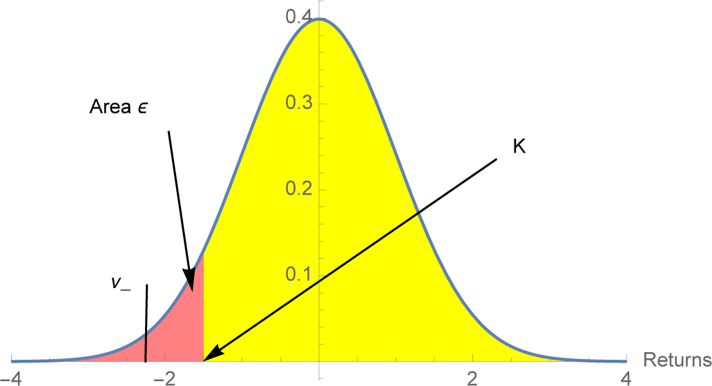
Suppose we assume X is Gaussian with mean μ and variance σ2. In principle it should be possible to satisfy the VaR constraints since we have two free parameters. Indeed, as shown below, the left-tail constraints determine the mean and variance; see Figure 1. However, satisfying the VaR constraints imposes interesting restrictions on μ and σ and leads to a natural inequality of a “no free lunch” style.
Let η(ϵ) be the ϵ-quantile of the standard normal distribution, i.e., η(ϵ) = Φ−1(ϵ), where Φ is the c.d.f. of the standard normal density ϕ (x). In addition, set
Proposition 1. If X ∼ N(μ, σ2) and satisfies the two VaR constraints, then the mean and variance are given by:
Moreover, B(ϵ) < −1 and limϵ↓0 B(ϵ) = −1.
Consider the conditions under which the VaR constraints allow a positive mean return
. First, from the above linear equation in μ and σ in terms of η(ϵ) and K, we see that σ increases as ϵ increases for any fixed mean μ, and that μ > 0 if and only if
, i.e., we must accept a lower bound on the variance which increases with ϵ, which is a reasonable property. Second, from the expression for μ in Proposition 1, we have
Consequently, the only way to have a positive expected return is to accommodate a sufficiently large risk expressed by the various tradeoffs among the risk parameters θ satisfying the inequality above. (This type of restriction also applies more generally to symmetric distributions since the left tail constraints impose a structure on the location and scale. For instance, in the case of a Student T distribution with scale s, location m, and tail exponent α, the same linear relation between s and m applies: s = (K − m)κ(α), where
, where I−1 is the inverse of the regularized incomplete beta function I, and s the solution of
.)
3.1. A Mixture of Two Normals
In many applied sciences, a mixture of two normals provides a useful and natural extension of the Gaussian itself; in finance, the Mixture Distribution Hypothesis (denoted as MDH in the literature) refers to a mixture of two normals and has been very widely investigated (see for instance Richardson and Smith (1995) [21]). H. Geman and T. Ané (1996) [22] exhibit how an infinite mixture of normal distributions for stock returns arises from the introduction of a “stochastic clock” accounting for the uneven arrival rate of information flow in the financial markets. In addition, option traders have long used mixtures to account for fat tails, and to examine the sensitivity of a portfolio to an increase in kurtosis (“DvegaDvol”); see Taleb (1997) [23]. Finally, Brigo and Mercurio (2002) [24] use a mixture of two normals to calibrate the skew in equity options.
Consider the mixture
An intuitively simple and appealing case is to fix the overall mean μ, and take λ = ϵ and μ1 = ν−, in which case μ2 is constrained to be
. It then follows that the left-tail constraints are approximately satisfied for σ1, σ2 sufficiently small. Indeed, when σ1 = σ2 ≈ 0, the density is effectively composed of two spikes (small variance normals) with the left one centered at ν− and the right one centered at at
. The extreme case is a Dirac function on the left, as we see next.
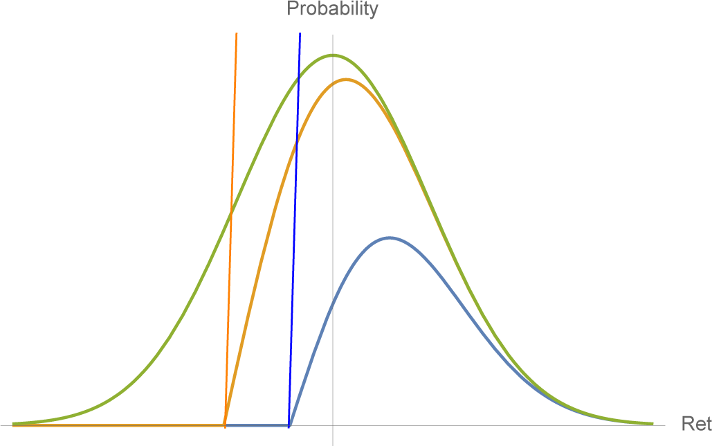
3.1.1. Dynamic Stop Loss, A Brief Comment
One can set a level K below which there is no mass, with results that depend on accuracy of the execution of such a stop. The distribution to the right of the stop-loss no longer looks like the standard Gaussian, as it builds positive skewness in accordance to the distance of the stop from the mean. We limit any further discussion to the illustrations in Figure 2.
4. Maximum Entropy
From the comments and analysis above, it is clear that, in practice, the density f of the return X is unknown; in particular, no theory provides it. Assume we can adjust the portfolio parameters to satisfy the VaR constraints, and perhaps another constraint on the expected value of some function of X (e.g., the overall mean). We then wish to compute probabilities and expectations of interest, for example
or the probability of losing more than 2K, or the expected return given X > 0. One strategy is to make such estimates and predictions under the most unpredictable circumstances consistent with the constraints. That is, use the maximum entropy extension (MEE) of the constraints as a model for f(x).
The “differential entropy” of f is h(f) = −f(x) ln f(x) dx. (In general, the integral may not exist.) Entropy is concave on the space of densities for which it is defined. In general, the MEE is defined as
where Ω is the space of densities which satisfy a set of constraints of the form Eϕj(X) = cj, j = 1, …, J. Assuming Ω is non-empty, it is well-known that fMEE is unique and (away from the boundary of feasibility) is an exponential distribution in the constraint functions, i.e., is of the form
where C = C(λ1, …, λM) is the normalizing constant. (This form comes from differentiating an appropriate functional J(f) based on entropy, and forcing the integral to be unity and imposing the constraints with Lagrange mult1ipliers.) In the special cases below we use this characterization to find the MEE for our constraints.
In our case we want to maximize entropy subject to the VaR constraints together with any others we might impose. Indeed, the VaR constraints alone do not admit an MEE since they do not restrict the density f(x) for x > K. The entropy can be made arbitrarily large by allowing f to be identically
over K < x < N and letting N → ∞. Suppose, however, that we have adjoined one or more constraints on the behavior of f which are compatible with the VaR constraints in the sense that the set of densities Ω satisfying all the constraints is non-empty. Here Ω would depend on the VaR parameters θ = (K, ϵ, ν−) together with those parameters associated with the additional constraints.
4.1. Case A: Constraining the Global Mean
The simplest case is to add a constraint on the mean return, i.e., fix
. Since
, adding the mean constraint is equivalent to adding the constraint
where ν+ satisfies ϵν− + (1 − ϵ)ν+ = μ.
Define
and
It is easy to check that both f− and f+ integrate to one. Then
is the MEE of the three constraints. First, evidently
- .
Hence the constraints are satisfied. Second, fMEE has an exponential form in our constraint functions:
4.2. Case B: Constraining the Absolute Mean
If instead we constrain the absolute mean, namely
then the MEE is somewhat less apparent but can still be found. Define f−(x) as above, and let
Then λ1 can be chosen such that
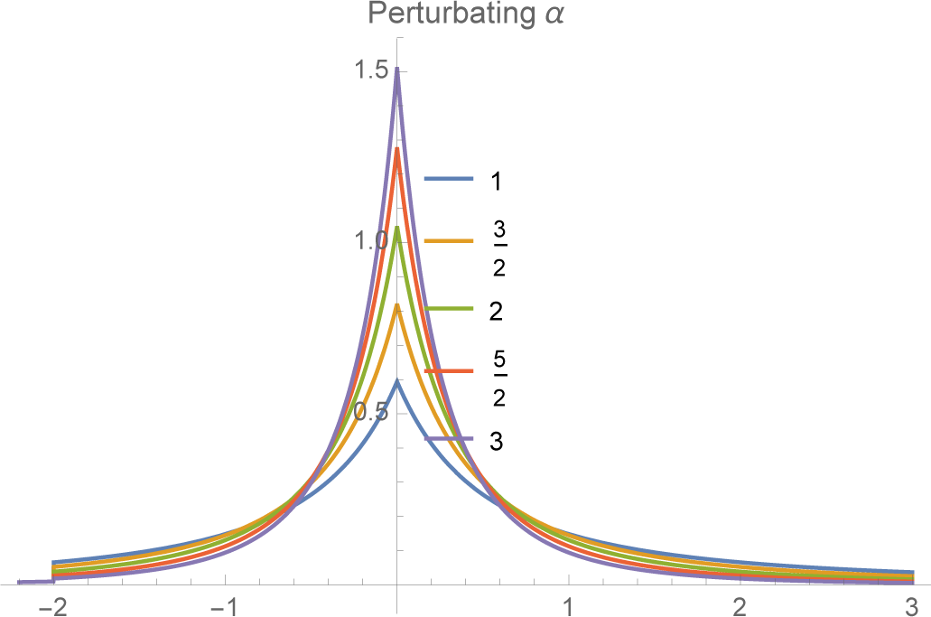
4.3. Case C: Power Laws for the Right Tail
If we believe that actual returns have “fat tails,” in particular that the right tail decays as a power law rather than exponentially (as with a normal or exponential density), than we can add this constraint to the VaR constraints instead of working with the mean or absolute mean. In view of the exponential form of the MEE, the density f+(x) will have a power law, namely
for α > 0 if the constraint is of the form
Moreover, again from the MEE theory, we know that the parameter is obtained by minimizing the logarithm of the normalizing function. In this case, it is easy to show that
It follows that A and α satisfy the equation
We can think of this equation as determining the decay rate α for a given A or, alternatively, as determining the constraint value A necessary to obtain a particular power law α.
4.4. Extension to a Multi-Period Setting: A Comment
Consider the behavior in multi-periods. Using a naive approach, we sum up the performance as if there was no response to previous returns. We can see how Case A approaches the regular Gaussian, but not Case C (Figure 7).
For case A the characteristic function can be written:
So we can derive from convolutions that the function ΨA(t)n converges to that of an n-summed Gaussian. Further, the characteristic function of the limit of the average of strategies, namely
is the characteristic function of the Dirac delta, visibly the effect of the law of large numbers delivering the same result as the Gaussian with mean ν+ + ϵ (ν− − ν+).
As to the power law in Case C, convergence to Gaussian only takes place for α ≥ 2, and rather slowly.
5. Comments and Conclusion
We note that the stop loss plays a larger role in determining the stochastic properties than the portfolio composition. Simply, the stop is not triggered by individual components, but by variations in the total portfolio. This frees the analysis from focusing on individual portfolio components when the tail—via derivatives or organic construction—is all we know and can control.
To conclude, most papers dealing with entropy in the mathematical finance literature have used minimization of entropy as an optimization criterion. For instance, Fritelli (2000) [25] exhibits the unicity of a “minimal entropy martingale measure” under some conditions and shows that minimization of entropy is equivalent to maximizing the expected exponential utility of terminal wealth. We have, instead, and outside any utility criterion, proposed entropy maximization as the recognition of the uncertainty of asset distributions. Under VaR and Expected Shortfall constraints, we obtain in full generality a “barbell portfolio” as the optimal solution, extending to a very general setting the approach of the two-fund separation theorem.
Acknowledgments
The authors thank the editor and the three anonymous referees for helpful comments.
Author Contributions
All three authors contributed to the research and have read and approved the final manuscript.
Conflicts of Interest
Although it may not technically represent a conflict of interest in the standard scientific sense, one of the authors (Taleb) reports that has been practicing variants of the “barbell” strategy throughout his trading career.
Appendix A
Proof of Proposition 1: Since X ∼ N(μ, σ2), the tail probability constraint is
By definition, Φ(η(ϵ)) = ϵ. Hence,
For the shortfall constraint,
Since,
, and from the definition of B(ϵ), we obtain
Finally, by symmetry to the “upper tail inequality” of the standard normal, we have, for x < 0,
. Choosing x = η(ϵ) = Φ−1(ϵ) yields ϵ = P (X < η(ϵ)) ≤ − ϵB(ϵ) or 1 + B(ϵ) ≤ 0. Since the upper tail inequality is asymptotically exact as x → ∞ we have B(0) = −1, which concludes the proof.
References
- Chicheportiche, R.; Bouchaud, J.-P. The joint distribution of stock returns is not elliptical. Int. J. Theor. Appl. Financ. 2012, 15. [Google Scholar] [CrossRef]
- Markowitz, H. Portfolio selection. J. Financ. 1952, 7, 77–91. [Google Scholar]
- Kelly, J.L. A new interpretation of information rate. IRE Trans. Inf. Theory 1956, 2, 185–189. [Google Scholar]
- Bell, R.M.; Cover, T.M. Competitive optimality of logarithmic investment. Math. Oper. Res. 1980, 5, 161–166. [Google Scholar]
- Thorp, E.O. Optimal gambling systems for favorable games. Revue de l’Institut International de Statistique 1969, 37, 273–293. [Google Scholar]
- Haigh, J. The kelly criterion and bet comparisons in spread betting. J. R. Stat. Soc. D 2000, 49, 531–539. [Google Scholar]
- MacLean, L.; Ziemba, W.T.; Blazenko, G. Growth versus security in dynamic investment analysis. Manag. Sci. 1992, 38, 1562–1585. [Google Scholar]
- Thorp, E.O. Understanding the kelly criterion. In The Kelly Capital Growth Investment Criterion: Theory and Practice; MacLean, L.C., Thorp, E.O., Ziemba, W.T., Eds.; World Scientific Press: Singapore, Singapore, 2010. [Google Scholar]
- Xu, Y.; Wu, Z.; Jiang, L.; Song, X. A maximum entropy method for a robust portfolio problem. Entropy 2014, 16, 3401–3415. [Google Scholar]
- Tsallis, C.; Anteneodo, C.; Borland, L.; Osorio, R. Nonextensive statistical mechanics and economics. Physica A 2003, 324, 89–100. [Google Scholar]
- Jizba, P.; Kleinert, H.; Shefaat, M. Rényi’s information transfer between financial time series. Physica A 2012, 391, 2971–2989. [Google Scholar]
- Hicks, J. R. Value and CapitalClarendon Press: Oxford, U.K, 1939; Volume 1946, 2nd ed. [Google Scholar]
- Tobin, J. Liquidity preference as behavior towards risk. Rev. Econ. Stud. 1958, 25, 65–86. [Google Scholar]
- Markowitz, H.M. Portfolio Selection: Efficient Diversification of Investments; Wiley: New York, NY, USA, 1959. [Google Scholar]
- Merton, R.C. An analytic derivation of the efficient portfolio frontier. J. Financ. Quant. Anal. 1972, 7, 1851–1872. [Google Scholar]
- Ross, S.A. Mutual fund separation in financial theory—the separating distributions. J. Econ. Theory 1978, 17, 254–286. [Google Scholar]
- Jaynes, E.T. How Should We Use Entropy in Economics; University of Cambridge: Cambridge, UK, 1991. [Google Scholar]
- Philippatos, G.C.; Wilson, C.J. Entropy, market risk, and the selection of efficient portfolios. Appl. Econ. 1972, 4, 209–220. [Google Scholar]
- Zhou, R.; Cai, R.; Tong, G. Applications of entropy in finance: A review. Entropy 2013, 15, 4909–4931. [Google Scholar]
- Georgescu-Roegen, N. The Entropy Law and the Economic Process; Harvard University Press: Cambridge, MA, USA, 1971. [Google Scholar]
- Richardson, M.; Smith, T. A direct test of the mixture of distributions hypothesis: Measuring the daily flow of information. J. Financ. Quant. Anal. 1994, 29, 101–116. [Google Scholar]
- Ane, T.; Geman, H. Order flow, transaction clock, and normality of asset returns. J. Financ. 2000, 55, 2259–2284. [Google Scholar]
- Taleb, N.N. Dynamic Hedging: Managing Vanilla and Exotic Options; Wiley: New York, NY, USA, 1997. [Google Scholar]
- Brigo, D.; Mercurio, F. Lognormal-mixture dynamics and calibration to market volatility smiles. Int. J. Theor. Appl. Financ. 2002, 5, 427–446. [Google Scholar]
- Frittelli, M. The minimal entropy martingale measure and the valuation problem in incomplete markets. Math. Financ. 2000, 10, 39–52. [Google Scholar]
Figure 1.
By setting K (the value at risk), the probability ϵ of exceeding it, and the shortfall when doing so, there is no wiggle room left under a Gaussian distribution: σ and μ are determined, which makes construction according to portfolio theory less relevant.
Figure 1.
By setting K (the value at risk), the probability ϵ of exceeding it, and the shortfall when doing so, there is no wiggle room left under a Gaussian distribution: σ and μ are determined, which makes construction according to portfolio theory less relevant.

Figure 2.
Dynamic stop loss acts as an absorbing barrier, with a Dirac function at the executed stop.
Figure 2.
Dynamic stop loss acts as an absorbing barrier, with a Dirac function at the executed stop.

Figure 3.
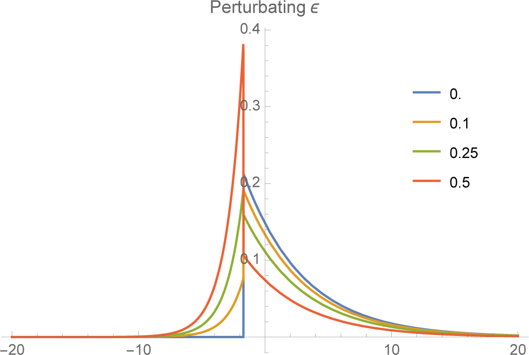
Case A: Effect of different values of ϵ on the shape of the distribution.

Figure 4.
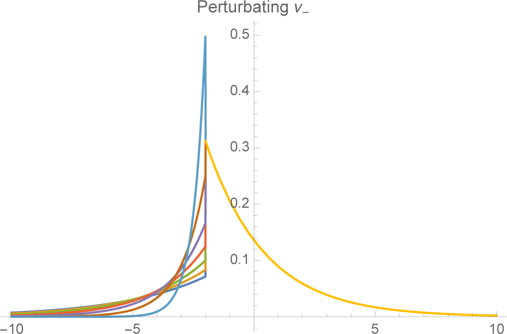
Case A: Effect of different values of ν− on the shape of the distribution.

Figure 5.
Case C: Effect of different values of on the shape of the fat-tailed maximum entropy distribution.
Figure 5.
Case C: Effect of different values of on the shape of the fat-tailed maximum entropy distribution.

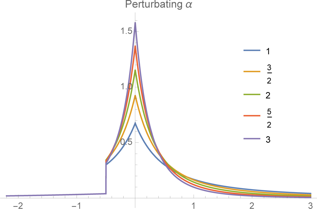
Figure 6.
Case C: Effect of different values of on the shape of the fat-tailed maximum entropy distribution (closer K).
Figure 6.
Case C: Effect of different values of on the shape of the fat-tailed maximum entropy distribution (closer K).

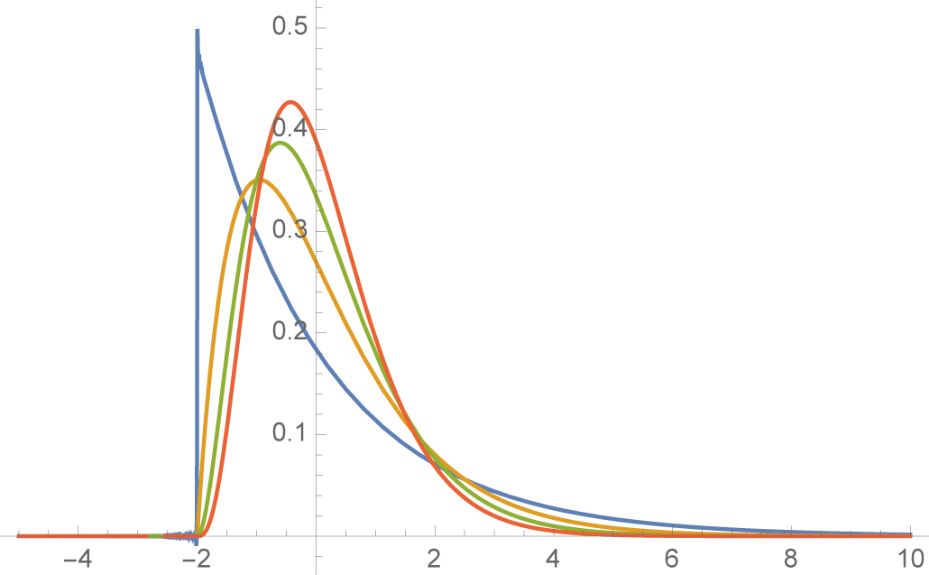
Figure 7.
Average return for multiperiod naive strategy for Case A, that is, assuming independence of “sizing”, as position size does not depend on past performance. They aggregate nicely to a standard Gaussian, and (as shown in Equation (1)), shrink to a Dirac at the mean value.
Figure 7.
Average return for multiperiod naive strategy for Case A, that is, assuming independence of “sizing”, as position size does not depend on past performance. They aggregate nicely to a standard Gaussian, and (as shown in Equation (1)), shrink to a Dirac at the mean value.

© 2015 by the authors; licensee MDPI, Basel, Switzerland This article is an open access article distributed under the terms and conditions of the Creative Commons Attribution license (http://creativecommons.org/licenses/by/4.0/).
Share and Cite
MDPI and ACS Style
Geman, D.; Geman, H.; Taleb, N.N. Tail Risk Constraints and Maximum Entropy. Entropy 2015, 17, 3724-3737. https://0-doi-org.brum.beds.ac.uk/10.3390/e17063724
AMA Style
Geman D, Geman H, Taleb NN. Tail Risk Constraints and Maximum Entropy. Entropy. 2015; 17(6):3724-3737. https://0-doi-org.brum.beds.ac.uk/10.3390/e17063724
Chicago/Turabian StyleGeman, Donald, Hélyette Geman, and Nassim Nicholas Taleb. 2015. "Tail Risk Constraints and Maximum Entropy" Entropy 17, no. 6: 3724-3737. https://0-doi-org.brum.beds.ac.uk/10.3390/e17063724