
Increase in Complexity and Information through Molecular Evolution

1
Institut für Theoretische Chemie, Universität Wien, Wien 1090, Austria
2
The Santa Fe Institute, Santa Fe, NM 87501, USA
Entropy 2016, 18(11), 397; https://0-doi-org.brum.beds.ac.uk/10.3390/e18110397
Submission received: 8 June 2016
/
Revised: 24 October 2016
/
Accepted: 7 November 2016
/
Published: 14 November 2016
(This article belongs to the Special Issue Information and Self-Organization)
Abstract
:Biological evolution progresses by essentially three different mechanisms: (I) optimization of properties through natural selection in a population of competitors; (II) development of new capabilities through cooperation of competitors caused by catalyzed reproduction; and (III) variation of genetic information through mutation or recombination. Simplified evolutionary processes combine two out of the three mechanisms: Darwinian evolution combines competition (I) and variation (III) and is represented by the quasispecies model, major transitions involve cooperation (II) of competitors (I), and the third combination, cooperation (II) and variation (III) provides new insights in the role of mutations in evolution. A minimal kinetic model based on simple molecular mechanisms for reproduction, catalyzed reproduction and mutation is introduced, cast into ordinary differential equations (ODEs), and analyzed mathematically in form of its implementation in a flow reactor. Stochastic aspects are investigated through computer simulation of trajectories of the corresponding chemical master equations. The competition-cooperation model, mechanisms (I) and (II), gives rise to selection at low levels of resources and leads to symbiontic cooperation in case the material required is abundant. Accordingly, it provides a kind of minimal system that can undergo a (major) transition. Stochastic effects leading to extinction of the population through self-enhancing oscillations destabilize symbioses of four or more partners. Mutations (III) are not only the basis of change in phenotypic properties but can also prevent extinction provided the mutation rates are sufficiently large. Threshold phenomena are observed for all three combinations: The quasispecies model leads to an error threshold, the competition-cooperation model allows for an identification of a resource-triggered bifurcation with the transition, and for the cooperation-mutation model a kind of stochastic threshold for survival through sufficiently high mutation rates is observed. The evolutionary processes in the model are accompanied by gains in information on the environment of the evolving populations. In order to provide a useful basis for comparison, two forms of information, syntactic or Shannon information and semantic information are introduced here. Both forms of information are defined for simple evolving systems at the molecular level. Selection leads primarily to an increase in semantic information in the sense that higher fitness allows for more efficient exploitation of the environment and provides the basis for more progeny whereas understanding transitions involves characteristic contributions from both Shannon information and semantic information.
1. Introduction
Biological evolution progressed and progresses by at least two different mechanisms: (i) Optimization of properties that are relevant for reproduction efficiency, which is measured in terms of fitness; and (ii) Major transitions that lead to the next higher hierarchical level of organismic complexity. Optimization gives rise to the enormous diversity of species and subspecies that mirrors the heterogeneity of environments. Evolutionary optimization follows the Darwinian mechanism of variation and selection [1]. This mechanisms is neither confined to living organisms nor to cells. In vitro evolution of molecules that are capable of replication and mutation, commonly RNA or DNA, follows essentially the same principles [2,3] and became an interesting tool of biotechnology in the design of biomolecules with predefined properties [4,5]. The hierarchical structure of biology and its objects is the most prominent result of major evolutionary transitions. In other words, the fact that we can recognize molecules, supermolecular aggregates, cell organelles, cells, organs, organisms, and societies in nature are the strongest hints that evolutionary transitions have led from one level of complexity to the next. Different major transitions share certain features but in general follow different mechanisms [6]. We illustrate by means of an example: Both transitions, (i) the transition from independent genes to a genome; and (ii) the transition from independent organisms to a symbiontic unit have in common that previously independent elements are integrated into the higher hierarchical unit and give up their autonomy—in total or partially—but the mechanism by which this is achieved is entirely different. In the first case, a sufficiently elaborate ligase joins the genes whereas the second case is built upon specific catalysis as will be discussed later on.
What can be said about the expected changes in information during the two evolutionary processes? First we need to define what features of information we are interested in here and it is appropriate to specify precisely the facets of the diverse meanings of information that we shall require. As outlined in Section 8 it is sufficient for our purpose to consider the simplest possible concepts: Shannon information, which increases with the coding capacity of the information carrier increases, and semantic information based on one or more evaluation criteria. In the simplest case of evolutionary relevance the obvious criterion is fitness being measurable in the form of the number of offspring or the rate parameter of growth. Darwinian optimization is accompanied by non-decreasing fitness corresponding to non-decreasing semantic information. Changes in Shannon information may occur but they are uncorrelated to changes in fitness. We shall encounter cases where increase in fitness is a result of decreasing chain length of RNA molecules [2] (see Section 8). The change in information during major transitions in more subtle. Although the relation between chain lengths and complexity of organisms is obscured by many side effects and anything but obvious even for phylogenetically close by lying species, there is no doubt that genome lengths have increased grosso modo in evolution. The coding capacity of organisms increases in major transitions where two or more carriers of genetic information come together to form a cooperative unit. The bacteria with the largest genomes after all are only partly overlapping in DNA length with the smallest protozoa and non-overlapping with multicellular eukaryotes [7]. At the same time the new units that were formed through integration of two or more simpler elements must compete successfully with their subunits as individuals and this implies that semantic information has increased in major transitions too (see Section 8).
A kind of minimal model (Figure 1 and [8,9]), which is derived from chemical kinetics of replication and which contains all essential features that are necessary for describing both optimization of fitness and transition to a higher hierarchical level, is presented in Section 2. At the same time the model is sufficiently simple to be accessible to mathematical analysis and stochastic simulation. The molecular players are understood as replicators being RNA or DNA molecules that are capable of replication, correct or error-prone in the sense of the sketch shown in Figure 2. By assuming suitable changes in the environmental conditions consisting of tunable accessibility of resources the model allows for a description of evolution on two hierarchical levels as well as the transition from the lower to the higher level. In particular, the occurrence of a transition is bound to the availability of sufficiently rich resources and it is possible to define a threshold below which cooperation between competitors does not happen and then no transition will take place. In accordance with the toy model we shall also consider the most simple concepts measuring changes in information: For Shannon information the contents of information is given by the chain length ν of the replicator. In other words we do not distinguish between coding regions, regulatory regions and other regions on the sequence, and we do not account for redundancies. Semantics assigns values to individual replicators, and consistent with the model the evaluation process uses as measure of semantic information the fitness of the phenotype as expressed by the replication rate parameter.
At present evolutionary optimization is fairly well understood. In fortunate cases the occurrence of optimization can be inferred from the fossil record but the inference is always indirect and the conditions under which it occurred are highly complex. Essentially the same is true for field observations in nature. The principle of Darwinian evolution, however, can be studied in evolution experiments with viruses [10] or bacteria [11,12] as well as in various cell-free in vitro assays. As mentioned already, in the first series of test tube experiments reported on evolution, which have been carried out with wild-type RNA of the Escherichia coli bacteriophage Qβ by Sol Spiegelman and his group [2,13], optimization of fitness was achieved through reduction of the virus genome to the absolutely necessary elements for reproduction: (i) a binding site for the enzyme Qβ-replicase; and (ii) a sufficiently rich secondary structure of both strands—plus and minus—in order to avoid duplex formation [14]. This reduction of the genome in the optimization process is made possible by the reaction medium, which supplies everything that is required for reproduction—except a template. Despite being the result of a complex many step template induced polymerization mechanism [15], RNA replication in case of excess resources and excess replicase follows a simple exponential growth characteristic and hence can be modeled by a simple autocatalytic reaction of the class . The interpretation of the kinetic data was supported by extensive computer calculations. One basic feature of biology is that all units are obligatory replicators. If an element fails to reproduce, it does not show up in future generations. The reproducing units contain genetic information in the form of DNA, only in case of viruses it might also be RNA serving the same purpose. Asexual reproduction comes closest to simple autocatalysis that will be used for reproduction kinetics in the minimal model. Important experimental achievements in the design of an RNA world as a plausible intermediate scenario for the origin of life were: (i) the discovery of catalysis by RNA molecules called ribozymes [16,17,18]; (ii) the design of autocatalytic networks of RNA molecules [19,20]; and (iii) the creation of an RNA based RNA replicase [21]. Experimental evolution found soon extensive applications in biotechnology: The SELEX method—selection of ligands by exponential enrichment—developed in the nineteen-eighties in the labs of Larry Gold and Jack Szostak [22,23] became an indispensable tool of molecular biology laboratories. In evolutionary biotechnology a whole repertoire of different techniques has been conceived and implemented for the design of biomolecules, for RNA-molecules [4] and for proteins [5].
Major transitions span a very broad spectrum from events described in origin-of-life models to the beginnings of human societies. One particular major transition, the origin of the eukaryotic cell is chosen for the purpose of illustration, because it is better understood than most other transitions and the toy model applied here comes relatively close to it. According to the interpretation of the fossil record exclusively prokaryotic life has covered the Earth for about 1.8 billion years, from 3.5 billion years to 1.7 billion years ago. Eukaryotic cells are not only much larger than prokaryotic cells, they have a much more complex structure with so-called cell organelles that according to the generally accepted hypothesis of endosymbiosis [24,25] were independently living organisms before the transition event. In the eukaryotic cell we have two or three reproducing units: (i) the nucleus; (ii) the mitochondria; and (iii) the chloroplasts in case of plant cells. The nucleus contains the major amount of the DNA of the cell but both mitochondria and chloroplasts have their own specific DNA, which encodes some of the organelle-specific proteins. Symbiosis of nucleus and organelle is, of course not the only form of symbiosis [26]. There are numerous examples of two or three-way symbiosis. Four member and higher symbiontic communities, however, are apparently very rare [27] (p. 71). We shall come back to this fact in Section 4, Section 7, and Section 9. Symbiosis characterizes the mutualistic interaction between species that is mutually beneficial. In the mutualistic system competition between elements is suppressed or, in other words, the individual components cooperate. For the minimal model we introduce cooperation in the form of catalytic action during replication, which in its simplest version has been formulated as catalytic hypercycle [28].
The third process that is basic to biological evolution is variation of phenotypic properties through changes in genotypes. It comes essentially in two forms: recombination and mutation. Consistent with the other simplifications of the minimal model presented here we consider exclusively point mutations, which are mutations in the simplest form: A point mutation changes the sequence of a DNA or an RNA molecules at a single position and already this minimal modification introduces a wide spectrum of possible variations into the phenotype that may range from no change to entirely new phenotypic properties. Introduction of mutation leads to formation of mutant distributions that become stationary after sufficiently long time. These stationary solutions are called quasispecies and have been extensively analyzed in the past [29,30,31,32]. They consist of a fittest variant, called the master sequence surrounded by its most frequent mutants weighted by fitness and by the distance to the master. Quasispecies evolve through the formation of fitter variants through mutation and restructuring of the mutant distribution around a new master sequence. The process of quasispecies evolution is visualized best as optimization or adaptive walk of a population on a fitness landscape. All three basic processes of biological evolution are are sketched in Figure 1.
2. A Minimal Model for Competition, Cooperation, and Mutation
The competition-cooperation-mutation (CCM) model [8,9] considers independent and catalyzed, correct and error-prone reproduction in a population of replicators or subspecies with . Stationary populations resulting from correct replication and mutation will be denoted as quasispecies and accordingly we shall use the term subspecies for individual replicators, which will be here always RNA or DNA molecules. A flow reactor (CSTR) is chosen as open system. The flow reactor is fed from a large reservoir filled with stock solution containing the material A at concentration where A stands for the whole set of materials that are required for reproduction. The mechanisms of reproduction and catalyzed reproduction in the flow reactor is encapsulated in chemical reaction equations:
Reaction (1a) supplies the material required for reproduction. A solution with A at concentration flows into a continuously stirred tank reactor (CSTR) with a flow rate r [35] (p. 87ff.) We remark that the deterministic kinetic Equation (4) were extensively studied under the simplifying assumption of constant population size [29,31,36]. The solution curves formulated in relative concentrations are identical for the CSTR and for constant population size but the stochastic system is unstable in the latter case [37]. The reactor operates at constant volume and this implies that the volume per time unit [t] of solution flowing into the reactor is compensated exactly by an outflow, which is described by the Equation (1d) and (1e) and concerns all molecular species, A and . More sophisticated flow reactors called chemostats and other experimental devices are also used to monitor and regulate available resources [38,39,40,41,42].
The notation for the rate parameters is chosen such that ambiguity is avoided: and with dimensions [Mt] and [Mt] refer to reactions in the flow reactor. For fitness and the cooperation parameter we use and , which have the dimensions [t] and [Mt]. Reactions (1b) model the processes of correct copying and mutation of replicators (Figure 2) and reactions (1c) finally include reproduction catalyzed by other replicators: (with ) supports the process of copying yielding either a correct copy of or a mutant . The terms (1c) introduce cooperation between otherwise competing subspecies. In the molecular interpretation acts as a specific catalyst for the reproduction process . In principle, we could have instead of n catalytic terms in (1c), because every molecule might act as catalyst in the reproduction of every other molecule but efficient and specific catalysis is rare and a meaningful model should not have more terms than required. Not all catalytic networks of replicators are stable in the sense that all subspecies survive in a cooperative organization. The presumably smallest stable functional organization is a hypercycle [36] and requires only n catalysts for n reactions: A sequence of catalytic interactions is closed to a loop,
and this introduces mutual dependence of all members of the hypercycle. If one subspecies, , dies out, the time-derivative of the previous species in the cycle, , becomes negative, vanishes and the entire organization collapses.
The molecular concept behind mutation in Equation (1b) is sketched in Figure 2: A template is bound to an enzyme initiating thereby a copying process that leads either to a correct copy, , or a mutant, . Equation (1c) describes the analogous reactions with subspecies () being a specific catalyst for the reaction. The mutation rates are summarized in the mutation matrix where is the frequency with which subspecies is obtained as an error copy of the template . Since the copying processes leading to the different subspecies are parallel reaction channels, which taken together exhaust all possibilities—each copy has to be either correct or incorrect—we have the conservation relation . Consistent with a minimal model is the assumption of uniform mutation rates: The mutation or error rate p is assumed to be independent of the nature of the mutated nucleotide residue as well as its position along the sequence. Then all elements of the mutation matrix are obtained from three parameters only,
The Hamming-distance counts the minimum number of consecutive point mutations required to produce as an error copy of .
Mechanism (1) is readily translated into kinetic differential equations with the molecular concentrations, and , as variables:
where we used the conservation relation in Equation (4b).
The competition-cooperation-mutation (CCM) model in the flow reactor has three internal and two external parameters. According to Figure 1 the three internal parameters are the fitness difference , the cooperation parameter , and the mutation rate . The external parameters are the concentration of resources in the stock solution, , and the flow rate, . The concentration of the material for reproduction in the stock solution, , is a measure of the available resources and determines the carrying capacity of the system. The flow rate r sets a limit to the time needed for reproduction events, because it is the reciprocal mean residence time of the solution in the reactor, , and allows for the approach towards thermodynamic equilibrium.
3. Competition and Cooperation
The dynamics of competition and cooperation with zero mutation is described by trajectories in plane (Figure 1). The mutation process is neglected simply by setting leading to where is the unit matrix. The equation for (4a) remains unchanged whereas the second equation simplifies to
For the low dimensional cases, , the kinetic equations are particularly simple and allow for straightforward mathematical analysis of steady states and bifurcations. Higher dimensional systems, , can also be handled analytically but the expressions become clumsy with increasing numbers of stationary states.
Steady state analysis reveals the long-time behavior of the system that is determined exclusively by stationary states, which are related by simple bifurcations, in particular transcritical and saddle-node bifurcations. Properly we start from Equation (4b’) and find for the stationary states:
Equation (4c) sustains two solutions for the steady concentrations of every subspecies: (i) extinction of given by ; and (ii) survival of is expressed by and requires
These two solutions for each stationary replicator concentration can be combined in principle to different steady states unless there are cases of incompatibility. As a matter of fact we have solutions since the concentration is obtained by means of a quadratic equation with two solutions. One of the two roots is always unstable [8,44]. For and three out of five states have regions of asymptotic stability in the -plane: (i) the state of extinction , ; (ii) the state of selection of , with ; and (iii) the state of cooperation , . Here, the concentration value is the root with the minus sign of the quadratic Equation (5)
with and . The second root corresponds to an unstable state . The state at which the only the less fit variant is present, , is unstable too.
For constant resources expressed by and initial conditions the long-time state of the system is uniquely defined. In Table 1 and Table 2 we list all stable stationary states for the cases and . The stationary coordinates of the states, or with , , and , are either constant or depend linearly on and/or r for all states except the cooperative state. In other words, the stationary states move along straight lines or are fixed in concentration space. Transitions between the individual solutions occur through transcritical bifurcations: The straight lines of two states, and , cross at the bifurcation points defined by and the stationary states exchange stability properties. The cooperative state is accompanied by an unstable state . For increasing flow rates r the expression under the square root vanishes and both states disappear at the critical value .
The system with sustains an additional stable stationary state between selection and cooperation where two species are present. We choose for the kinetic parameters: and . This choice simplifies the discussion to some extent because no distinction of subcases is required. We obtain and denote the state as state of exclusion of . For higher dimensionality, , further states with three and more coexisting species and other species missing will be observed. Eventually we find the following ordering of stability ranges of stationary or quasi-stationary states with increasing resources expressed as -values:
The state of cooperation is an asymptotically stable stationary state for as it is for provided the flow rate is below the critical value .
In the pure hypercycle equation—Equation (4) with , , and —weakly damped oscillations around an asymptotically stable stationary state are observed for . For the cooperative state is unstable [45] and the ODE (1) sustains a stable limit cycle [46]. As we shall show in the next section stochasticity introduces instability into hypercycle dynamics of cooperative systems with . In the CSTR the stationary concentration of A at the state of cooperation is not constant but results from the quadratic equation
Interestingly, Equation (5) depends on n only through the summations in ψ and ϕ, and hence the equation is valid for arbitrary n. The second solution belongs to an unstable state (see e.g., [44] (pp. 674–675)) and is important in the context of a saddle-node bifurcation at which the states and disappear above the critical flow rate [9].
The model for cooperation in the CSTR by means of hypercycles deserves additional attention because it is accessible to full analytical treatment. As in the case of constant concentrations of a and the nature of the solution curves and stationary states depends crucially on the number of molecular species n. Since the dimensions of the rate parameters are [Mt] and [Mt], respectively, the choice of sufficiently high concentrations allows for the neglect of terms containing against those with in Equation (4b’). Then we are dealing with pure hypercycle dynamics in the flow reactor as it has been studied analytically before [44]. The mechanism and the kinetic differential equations are obtained from Equations (1) and (4) by putting . With a simple transformation of variables, , with , which has been denoted characteristically as barycentric transformation [47,48,49], the stationary point inside the concentration simplex can be shifted into the center. From follows that all stationary concentrations have the same value , and can be calculated from Equation (5) by setting . Then, for we obtain two solutions of the quadratic equation:
The solution with the plus sign corresponds to the solution with the minus sign for A, . The stability of the central stationary point follows from the eigenvalues of the Jacobian matrix:
The two solutions correspond to the two steady states and , respectively, and inspection of Equation (7) shows that is always unstable because of the plus sign, . The eigenvalue is always negative and stability or instability is therefore determined by the roots , which represent the complex roots of one except that does not exist as a solution here. Accordingly, is asymptotically stable for and . The case is special: The linearization around the stationary point is a marginally stable center with two eigenvalues with zero real part, . There is however a higher order term, which renders the state asymptotically stable. Integration of the differential Equation (4) with and yields indeed weakly damped oscillations [45]. For the central point is unstable and the system sustains a stable limit cycle [46], which manifests itself through undamped oscillations.
The ODEs (4) combine competition and cooperation kinetics and are appropriate candidates for modeling transitions from Darwinian selection to stable symbiosis. At the same time it seems that nothing in the model can be omitted without loosing the capability to describe such a transition and therefore we intend to conjecture that it is also the simplest model possible. Despite its simplicity the model provides a straightforward explanation for the emergence of cooperation in a world of competitors triggered by increasing resources.
4. Stochastic Kinetics in the Competition-Cooperation System
The most natural way for considering stochasticity in chemical reactions and reaction networks is to write down and analyze the chemical master equation corresponding to mechanism (1). In order to distinguish particle numbers and concentrations we use upper case letters for former: and . The probabilities are expressed by and with , and finally the multivariate master equation of the competition-cooperation system is of the form
The index set is denoted by and , etc. Since the derivation of the master equation assumes that chemical processes occur one at a time all jumps involve single elementary steps and the reactions in the mechanism (1) change particle numbers by , we apply here a notation in shorthand for changes of the index set for reaction ,
Although it is not difficult to write down a multivariate master equation, the derivation of analytical solutions is successful only in exceptional cases, for example for networks of monomolecular reactions [50,51]. An alternative strategy for studying chemical master equations is computer simulation through sampling of trajectories. The theoretical background for trajectory harvesting has been laid down by Andrey Kolmogorov [52], Willy Feller [53], and Joe Doob [54,55]. With the incoming of electronic computers, simulations of stochastic processes became possible. The conception, analysis, and implementation of a simple and highly efficient algorithm by Daniel Gillespie [56,57,58] provided a very useful tool for investigations of stochastic effects in chemical kinetics. Here we present some results, which illustrate the differences between deterministic and stochastic solutions of the transition model.
A typical trajectory with is shown in Figure 3. In order to facilitate the analysis we start with an empty reactor, , that contains only the autocatalytic molecules in seeding quantities. These initial conditions allow for the distinction of four phases of the stochastic process. The inflow of stock solution with results in a rapid increase of the number density of A molecules (phase I). In contrast to deterministic reaction kinetics knowledge of parameter values and initial conditions are not sufficient for correct predictions of the final state: In phase II random events guide the system either towards the absorbing state of extinction () or to one of the three quasi-stationary states (, or ). In phase III the system approaches the long-time state and eventually in phase IV we observe the trajectories fluctuating around the deterministic values of the corresponding stationary states (, , or ).
The existence and uniqueness conditions for the solutions of ODEs apply to the kinetic Equation (4b) and we are dealing with a unique long-time behavior for precisely defined parameters and initial conditions. In contrast to the solution of a kinetic differential equation the outcome of stochastic trajectories with identical parameters and initial conditions need not be unique. Indeed the example of the trajectory shown in Figure 3 shows a representative case of one class—the class converging to —whereas trajectories may converge to any of the four stationary states, the absorbing state and the three quasi-stationary states , , and . By trajectory sampling we calculate the probabilities for ending up in a particular state. In Table 3 we present the results for counting final states for different initial conditions and sets of parameter values. Seeding values of five molecules and each and a sufficiently large value of are enough to obtain almost certain convergence of the stochastic trajectories to the cooperative state .
The interpretation of the individual values in Table 3 is straightforward. The more seeding molecules of a given species we have, the less likely it is eliminated during the random phase II. We observe selection of both replicators and , and the presence in more copies overrules the difference in fitness values—at least in the example shown here. One might argue: “When particle numbers of five are already sufficient to come close to the deterministic results why worry about stochastic effects at all?” This argument were valid, were there not the fact that every mutant inevitably has to begin with a single copy, and in the early evolutionary phase of a newly created molecular species stochasticity is always important. Interestingly, the probability to become extinct depends primarily on the sum of the seeding molecules, , and not so much on the distribution over the two initial states. The interpretation is straightforward: The probability that all molecules () are diluted out of the reactor before they are replicated does not depend on the particular subspecies, or .
Stochasticity in competition-cooperation dynamics of systems with shows additional features that are not present in the deterministic solutions of the kinetic equations. The interpretation is easier if one considers first pure hypercycle dynamics, , for . The kinetic equations sustains two states: (i) extinction with and (); and (ii) cooperation consisting of an unstable state surrounded by a stable closed orbit resulting in oscillating variables [46]. The cooperative state is unstable in the stochastic process as well. Strong uncompensated fluctuations undergo autocatalytic self-enhancement for , the stochastic variables exhibit noisy oscillations and the amplitudes of the oscillations grow with time until one subspecies, say , dies out. Then we have and accordingly vanishes followed by decreasing concentrations of until it dies out, then vanishes and so on. In the pure hypercyclic system the whole population dies out with the disappearance of (). The sequence of extinction obviously is the same as the sequence of hypercyclic catalysis (2). The four dimensional system () is more subtle: At small population sizes the situation is the same just as described for but in large populations it may take very long time before the concentration of one subspecies becomes zero and then we observe oscillation of the concentrations of all subspecies with fluctuating frequencies and amplitudes. Since every new species in biological evolution has to start ultimately from very small population sizes (), we may expect that in reality cooperative systems with four members are unstable like the larger ones.
In essence, the addition of first order autocatalytic reaction terms, , changes the dynamics only in one aspect (Figure 4): Frequent possible outcomes are not only the two states extinction and the cooperative state but also the n selection states (). The last remaining subspecies in the sequence of extinction from above, , and A together form a quasi-stationary state. Since every subspecies may be wiped out first, every possible selection state , can result as final outcome.
In summary, stochasticity introduces two major changes into the competition-cooperation system: (i) Fluctuations allow for the choice between several final states of the stochastic process with identical parameters and initial conditions; (ii) cooperative systems with five and more partners are unstable and lead to random selection of one subspecies or extinction; and (iii) the case is intermediate in the sense that the quasi-stationary cooperative state is long-lived as with and for sufficiently large population sizes but unstable in small populations like the systems with .
5. Competition, Mutation and Quasispecies
Optimization of mean fitness may occur through competition and mutation in evolving populations. The competition-mutation system (coordinate plane ) is studied in the CSTR and the equations result from mechanism (1) through neglect of second order autocatalysis (1c), . In order to illustrate the problem with the simplest possible case we begin with correct replication, . Then we are left with the kinetic differential equations
Equation (9) sustains two stationary states: (i) the state of extinction, , characterized by and ; and (ii) the state resulting from natural selection, , of the uniquely defined subspecies with highest fitness, with , since we do not consider neutral evolution [34] here where two or more subspecies have identical largest fitness values. The state fulfils the conditions
In order to reveal the relation between selection and fitness optimization we consider the mean replication rate with and its time derivative,
The concentration of A is positive, and the variance of any distribution is a nonnegative quantity too, , where the equal sign requires a homogeneous population, and , and hence is always fulfilled. It is, of course, possible to choose but then we have and in the next instant would be fulfilled. Equation (9d) states that the mean fitness is always increasing except at its maximum , which is the stationary state . Hence the mean fitness of populations is optimized during the process of selection in the flow reactor.
Equation (9b) can be rewritten and interpreted differently [59] (pp. 29–32): For every replicator we define a specific growth function that describes unconstrained growth, , and an unspecific constraint , which is the same for all replicators:
In the flow reactor, for example, the constraint fulfils: . In more elaborate reactors as far as the experimental implementation is concerned other constraints lead to expressions that are more complicated to write down but often easier to analyze. Summation over all subspecies yields an ODE for the total concentration of replicators:
which can be used to calculate from known and vice versa:
Stationarity in the total concentration, , allows for an expression of the constraint in terms of the growth functions: . This constraint—often called constant concentration or constant organization—is particularly useful for the analysis of replicator equations [36,45,60]. Insertion into Equation (9e) yields
Next we introduce normalized concentrations, , with and into Equation (9e) and the ODE for becomes
Summation of normalized concentrations yields . Accordingly we find for the constraint and obtain
It is worth noticing that Equation (9g) does not contain explicitly the constraint and hence it is valid for almost all cases: The evolution of the population described in normalized variables is independent of the constraint as long as the population size does neither become zero nor approach infinity. An implicit dependence of the rate Equation (9g) on the constraint is nevertheless given through the concentration . In case the growth functions are homogeneous functions of degree λ in x, we find
and the ODE in normalized concentrations takes on the form:
Since Equation (9h) and (9e’) are identical apart from the factor , which can be absorbed in the time axis as long as and are fulfilled. Two cases can be distinguished: (i) , the stationary states of both equations are the same and so are the trajectories on the concentration simplex but the solution curves differ by the time factor ; and (ii) , the factor containing time and total concentration is one and thus time independent, and the two equations do not only have the same stationary states but also identical solution curves. In other words the course of competition and selection is the same in stationary and growing populations. Darwinian optimization is based on first order autocatalysis characterized by homogeneous growth functions with . Hypercycle dynamics uses homogeneous growth functions with and the internal equilibrium in the growing system is identical with the stationary state approached at constant concentration. We remark that the growth functions in the competition-cooperation system, with , are not homogeneous and the regularities reported in this paragraph do not apply therefore.
Evolutionary optimization requires more than selection. Variation of genotypes is a conditio sine qua non for the Darwinian mechanism and in the spirit of the as simple as possible CCM-model we introduce point mutation (Figure 2) as source of variation. In order to study competition-mutation dynamics we set in the mechanism (1) and obtain the kinetic differential equations
The growth functions are homogenous and linear in and hence the equations in conventional and normalized concentrations, and , are the same, and have identical solutions. The stationarity condition, , yields again two solutions (i) the state of extinction and (ii) the state of quasispecies selection at with [30]. The two states are related by a transcritical bifurcation at . The state of selection, , is asymptotically stable for small flow rates, or sufficiently large resources . Extinction occurs at high flow rates, , and small resources . The problem is not yet solved completely because the stationary mutant distribution, the quasispecies , is needed for the calculation of . The quasispecies is conventionally obtained through the solution of an eigenvalue problem and we shall briefly sketch this procedure here. Other approaches make use of techniques developed in the statistical mechanics of magnetic systems [61,62,63,64] (for a recent update see [65]).
Because of Equation (9h) with the solutions approaching the state of quasispecies selection are the same at constant or variable population sizes and without loosing generality the replication-mutation problem can be and has been solved at constant resources as well as constant population sizes [29,30,31] (for a recent review see [32]). The constant concentration of A is absorbed in the fitness value . We mention here only the most prominent results, which are relevant for the forthcoming discussion of changes in the information content of a population. The quasispecies is obtained in form of the largest eigenvector of the value matrix ,
which is a product of the mutation matrix and a diagonal matrix containing the fitness values of all subspecies. The eigenvalue problem is of the form
Vectors are assumed to be row vectors here and, in particular, the symbol ‘’ means transposed and indicates a column vector.
The matrix is either positive or at least nonnegative and irreducible, the conditions for the applicability of the Perron-Frobenius theorem [66] are fulfilled, and hence the largest eigenvalue is a non-degenerate eigenvalue and the corresponding eigenvector, the quasispecies , which represents the long-time solution of the competition-mutation problem, has exclusively positive components. In other words, all subspecies are present at the stationary state and no mutant vanishes in the process of natural selection combined with error-prone reproduction. The most frequent subspecies in the quasispecies is called the master sequence, . Often but not always it is the variant with the highest selective value, . In case the replication accuracy is the same for all subspecies, —as it occurs, for example, with the uniform error rate assumption—the sequence with the largest selective value is identical to the sequence with highest fitness. As we shall show in Section 6 this need not necessarily mean that the fittest sequence or the sequence with the largest selective value is the master sequence. The quasispecies consists of the master sequence and a mutant cloud surrounding it where the width of the cloud depends on the distribution of fitness values and the mutation rates.
How is Darwinian natural selection changed by the inclusion of mutations? The answer is readily given in mathematical terms. Frequent mutations couple individual subspecies to clans that are selected together and the clan, which reproduces with maximal efficiency is the dominant eigenvector of the value matrix . Eigenvectors corresponding to the other eigenvalues are less efficient since we have
and after sufficiently long time only the term containing is important, since the time dependent weighting factors of the contribution of the eigenvectors are: . All eigenvectors except have positive and negative components and are positioned outside the physically reachable concentration space defined by nonnegative concentrations . Population dynamics can be visualized as a process in the space spanned by the eigenvectors :
where is a Cartesian eigenvector in the direction of . Indeed rewriting replication-mutation dynamics in terms of the eigenvalues and eigenvectors of yields a kinetic differential equation that looks identical to the mutation-free case with the fittest subspecies being replaced by the quasispecies . The stationary solutions are defined by and are—as required—independent of time and initial conditions. The stationary mean fitness, , is the maximal mean fitness, which the population can achieve at mutational equilibrium. It fulfils necessarily , where the equal sign corresponds to no mutation and holds for a homogeneous population of master sequence. In other words, the maximal fitness can be obtained only for vanishing mutation rates . Obviously, the optimization theorem of the mean fitness derived for error-free replication is not valid any more and trajectories along which mean fitness is decreasing or non-monotonously changing are easily found. According to Equation (10e) the time dependence of the population is given by a superposition of exponential functions with the eigenvalues . After sufficiently long time—when the system is close to the stationary state—only the largest eigenvalue and the corresponding eigenvector are important.
Exact solutions in closed form are not available but phenomenological expressions for the purpose of illustration can be derived through three simplifying assumptions [29,32]:
The fact that individual fitness values do not enter the Equation (11a) is a results of the assumption of a single peak fitness landscape.
- (i)
- A single-peak fitness landscape is applied that assumes equal fitness for all mutants and a higher fitness for the master sequence (Section 6).
- (ii)
- A uniform mutation rate per site and replication event, p, is assumed. In other words the frequency of mutation is assumed to be independent of the nature and the position of the mutated nucleotide. The mutation matrix is largely simplified by the uniform error rate assumptionThe Hamming-distance counts the minimum number of point mutations needed to produce as an error copy of .
- (iii)
- Mutational backflow in the kinetic differential Equation (10) is neglected. We rewrite Equation (10b) for and partition in two contributions coming from correct copying of the template and from incorrect copying of all other with , and neglect the second term:
The stationary frequency at which a given subspecies is present in the quasispecies is a function the mutation rate p and the degree of relatedness to the master sequence expressed by the Hamming distance. There is, of course, also a dependence on the difference in fitness values, , which is encapsulated here in the superiority of the master sequence,
and which will be discussed in detail in Section 6. The quantity is the mean fitness of all sequences except the master. Since the stationary concentration of mutants decreases fast with increasing Hamming distance from the master sequence and the width of the distribution increases with increasing mutation rate p. The most prominent result of quasispecies theory is the existence of a sharply defined error threshold and follows directly from Equation (11a). All components of the quasispecies contain a common factor , which becomes zero at the critical mutation rate , where the chain length of the polynucleotide template is denoted by ν and is the superiority of the master sequence defined above. The approximation applied in Equation (11a) assumes equal fitness of all mutants. This assumption can be relaxed in the sense that all fitness values are different without loosing the existence of a sharp error threshold (see Section 6 and [32]).
The existence of a critical error rate or error threshold can be interpreted heuristically in straightforward way: Mutation has the consequence that a certain fraction of the copies of the master sequence, , are less fit than the parent subspecies. This fraction apparently increases with increasing mutation rate p whereas the mean fitness of the stationary population decreases. There is a—very high—mutation rate at which the incorporations of correct or incorrect digits are equally probable—for binary sequences this occurs at an error rate of : At this point all mutants are produced with equal probability and the stationary distribution of subspecies is the uniform distribution. Properly one can characterize reproduction at such a high level of inaccuracy as random replication. If an error threshold exists, the transition from the ordered regime of a structured quasispecies to a uniform distribution produced by random replication occurs to a very good approximation already at much lower error rates: . In other words, in systems with error thresholds the point of random replication is widened to a broad zone .
6. Sequence Space, Fitness Landscape, and Population Dynamics
Understanding evolution is facilitated enormously by the application of two fundamental concepts: (i) sequence space; and (ii) fitness landscape. Nucleic acids are visualized as carriers of genetic information, the sequence or genotype space is a point space, and every nucleic acid sequence is represented by a point. The distance between two sequences and is the Hamming metric [29,67,68]. It should be mentioned that the idea of a sequence space for proteins originated about the same time [69].), which represents the minimal number of point mutations that are required in order to interconvert the two sequences. The notion of fitness landscape goes back to the population geneticist Sewall Wright [70,71]: A fitness value is assigned to every point in sequence space and the resulting object is a landscape over a high-dimensional support. Sequence spaces are huge—the number of possible sequences of chain lengths ν over an alphabet with κ digits is and this amounts to for small natural nucleotide sequences of length . In reality sequence spaces can never be fully covered by populations, which only in exceptional cases can be as large as individuals. Thermodynamics on the other hand assumes equal distribution of molecular species over all degrees of freedom and the deterministic approach is based on the assumption that concentrations may become arbitrarily small. In chemical kinetics of replication and mutation (Equation (10) and Figure 2) qualitatively the same situation arises by the assumption that all reaction channels, , are populated according to their weighting factors . This is far away from any real situation where we have either one molecule or none and the usage of a discrete model is indispensable. A real population covers only a tiny part of sequence space—a typical distribution of virus genotypes, for example, consists of (i) a master sequence; (ii) a core of frequent mutants, which are present almost all the time; and (iii) mutants at the periphery, which “come and go”. Master sequence and its frequent mutants may be described by the deterministic quasispecies equation restricted to the area of sequence space that is covered by the core. We shall use the term local quasispecies here in order to express the fact that optimization of fitness is restricted to a small region in sequence space. The periphery, accordingly, cannot be modeled properly unless fluctuations are taken into account.
A snapshot of an evolving population will most probably catch a local quasispecies. New mutants are formed and the selective value of the majority of them does not exceed that of the current master sequence , . Once in a while a mutant is formed, which has a higher selective value than the current master, . Provided the new sequence is not lost during a stochastic initial period, a new local quasispecies centered around with . Computer simulations [72,73,74,75,76] have shown that quasispecies evolution as sketched in Figure 5 follows regularly a two phase process: (i) During the quasi-stationary phases along fitness plateaus the master sequence stays the same, the mean fitness is approximately constant and the population broadens in sequence space; and (ii) a plateau phase ends by the advent of a fitter mutant, the width of the population shrinks instantaneously, the mean fitness increases and a new mutant cloud builds up around the new master sequence . Such two phase processes—broadening of the population though the formation of a mutant cloud around a master through spreading by stochastic drift, and narrowing of the population as a consequence of the transition to a new master—is repeated over and over again as long as the global optimum has not been reached. Because of the enormous size of sequence space a typical trajectory will not be able to come even close to the optimum and therefore the evolutionary process is practically open ended in most cases. The difference between the fitness and the selective value of the master sequence, , is a quantity that depends exclusively on the properties of the master sequence and hence is different from the mutation load that measures the fitness of the master sequence relative to the mean fitness of the population: . Both quantities become zero in a homogeneous population of the master sequence. The evolutionary sequence of selective values is determined by the inequality
Fulfilling the equals sign in the last inequality requires vanishing mutation rates, .
How do realistic fitness landscapes look like [32] (pp. 62–75)? The investigation of biopolymer structures and functions as well as extensive works on pathogenic virus populations revealed three generic features of fitness landscapes in recent years [77,78,79,80]: (i) Realistic fitness landscapes are high dimensional—in a polynucleotide sequence of length ν all ν positions can be varied independently and the sequence space is a discrete ν-dimensional object with κ points in every direction; (ii) fitness landscapes are rugged in the sense that a small change in the sequence may cause dramatic fitness changes or no change at all; and (iii) neutrality implying that several or many sequences have the same selective value. Figure 6 sketches an adaptive walk and shows how a neutral segment of the walk may bridge an otherwise unsurmountable obstacle for the walk on a rugged landscape. The sketch at the same time suggests that both neutrality and ruggedness are required for evolution: Without sufficient neutrality adaptive walks would be trapped at some low-lying nearby peaks. If the peak is a member of a neutral network, however, the population can circumvent the trap by random drift in another direction and reach a point from which the adaptive walk can be continued. Ruggedness is a consequence of the generic relations between biopolymer sequences, structures and functions (For details of sequence-structure-function mappings of RNA molecules see [76,81,82]). It creates a multitude of local fitness optima and provides the basis for diversity in nature and adaptation to environmental changes.
Despite spectacular successes in the experimental determination and empirical modeling of fitness landscapes (see, for example, [78]) detailed information on sufficiently large parts of fitness landscapes is still missing. Accordingly, almost all studies were made with more or less simple model landscapes. Many results of quasispecies theory were derived by means of largely simplified landscapes and an important question concerns the general validity of these findings. As representative examples we mention here three landscapes. A very simple but nevertheless frequently used example is the single peak landscape:
with . It has only two fitness values, the fitness of the master sequence and the fitness value shared by all sequences except the master. It was used in the calculation of the analytical expression for the error threshold and we ask now whether or not error thresholds are also found on more general landscapes.
For this goal we construct more realistic landscapes that allow to apply different fitness values for different individual sequences. The lack of sufficiently detailed empirical data forces us to use some random input, which we create by superposition of random scatter upon single peak landscapes. Because we aim at mimicking landscapes that are ultimately derived from biopolymers, such landscapes are called realistic random landscapes (For another class of empirical random landscapes see, for example, the Nk-model [83,84]):
where is the output of a pseudorandom number generator drawing numbers from a uniform distribution on the interval , , which had been started with the seeds s. The parameter d allows for tuning the degree of randomness. The value implies the single peak landscape with no random scatter at all and yields a band with fully developed random scatter covering the entire range .
The third example is a realistic random landscape with a tunable degree of neutrality, λ. Neutrality is incorporated into realistic random landscapes in straightforward manner: The fitness value is not only assigned to the master sequence but to all sequences with pseudorandom numbers where is a tunable degree of neutrality:
It is easy to see that yields the non-neutral landscape and results in completely flat landscape. Evolution on the flat landscape is described by the neutral theory of evolution developed by Motoo Kimura [34].
One general result derived from rugged fitness landscapes with resolution to individual sequences concerns the existence of an error threshold. Compared to the single peak landscape the position of the threshold is shifted towards smaller p-values with increasing random scatter d and this observation is readily explained by the fact that the difference between and the next highest fitness values is reduced with increasing d [32] (pp. 98–114). There are, however, rather smooth simple landscapes, which do not sustain error thresholds [32,85]. Neutrality, in general, does not prevent the existence of error thresholds. Single master sequences may be replaced by cluster of closely related neutral sequences [32]. Another relevant finding concerns landscapes with high degree of ruggedness, : Depending on the distribution of fitness values controlled by the seeds of the pseudorandom number generator we observe two cases: (i) strong quasispecies where the master sequence stays the same in the entire range for , and (ii) standard quasispecies, which undergo one or more transitions where the master sequence changes at certain critical mutation rates [32].
The necessary and sufficient condition for the occurrence of a transition between quasispecies with different master sequences is crossing or avoided crossing of two eigenvalues at the transition point [86]. The eigenvalues as functions of the mutation rate p are accessible only by numerical calculation but the existence of a transition can be made plausible by inspection of the two kinetic differential equations for the two potential master sequences and (A rigorous derivation of the condition for transitions between quasispecies is found in [87]). We mention also that transitions between quasispecies were rediscovered thirteen years later by Claus Wilke et al. in numerical simulation by means of digital organisms [88] and characterized by the catchphrase survival of the flattest where flatness refers to the fitness landscape:
Which of the two candidates, or , becomes the master sequence depends on the difference between the two differential quotients at the point , as expressed by the two differences and . If is positive, is (very likely to become) the master sequence (As said the transition occurs at a crossing or avoided crossing of two eigenvalues and and the difference discussed here is the leading term in the difference of the eigenvalues, which determines almost always (but not always) the exact behavior.), whereas is a very strong indication for being the master sequence. Within the uniform error rate assumption we have . At the two differences have the values , and since iff , and hence is the master sequence. Next we increase p at constant d, and Q as well as become smaller, whereas at the same time the terms containing increase in absolute value. We need to consider only cases where for because otherwise, for , will be always positive and no transitions between quasispecies, , can occur. For the difference becomes smaller with increasing mutation rates p and it may become negative before the population reaches the error threshold at and then we observe a transition between two different quasispecies.
The role of the intensity parameter d of random scatter of fitness values is readily analyzed. As a reference we consider the case , the single peak landscape. Straightforward calculations yield and , and accordingly we obtain , and no transitions are possible on single peak landscapes. The influence of a distribution of fitness values with instead of the single value of the single-peak landscapes can be predicted straightforwardly: Since in Equation (13b) is independent of the fitness scatter d, and , which evidently has to lie above the average , is increasing with increasing scatter, the difference will decrease with increasing d. Consequently, the condition for a transition between quasispecies can be fulfilled at lower p-values the larger d is and we expect to find one or more transitions below the error threshold . Numerical calculations show that is commonly needed for the occurrence of transitions [32].
7. Cooperation and Mutation
The question to be handled in this section concerns the influence of mutation on a dynamical system showing cooperation between subspecies. The influence of mutation is particularly important in oscillating stochastic systems with high probability of extinction. Intuitively one would guess that high mutation rates could compensate for extinction through reintroduction of the missing subspecies. Whether or not this is the case has been be investigated by computer simulation (Schuster, P., unpublished results, 2016), because mathematical analysis of the hypercycle equation with mutation is rather involved. As we have seen in Section 4 four membered hypercycles with small population size and all hypercycles with five or more members () are endangered by extinction. Self-enhancing stochastic oscillations increase in amplitude until a subspecies vanishes and the whole system dies out. In the two examples shown in Figure 7 mutations prevent the system from extinction several times but the mutation rate parameter p is not large enough to sustain the population with probability one for arbitrarily long time. Figure 8 shows an episode where two subspecies are successfully replaced by mutation.
Cooperation-mutation dynamics is based on the mechanism (1) with leading to the differential equations
A mutation matrix with the elements calculated from the mutation rate parameter p and a distance between the subspecies has to be defined. In case of the quasispecies it has been natural to choose the conventional sequence space as reference and to apply the uniform error rate model (3). Accordingly the appropriate choice for is the binary sequence space with chain length . For there exists no analogue of a sequence space and we choose a mutation matrix that is built upon a pentagram (see caption to Figure 7). As before in the quasispecies equation the ODE for A does not depend explicitly on the mutation rate p but there is, of course, an implicit dependence via the concentration variables . The internal parameters on the cooperation-mutation plane (Figure 1) are the rate parameters or and the mutation rate p. Since the dynamics of hypercycles remains essentially unchanged in a barycentric transformation we assume equal rate parameters, or (), without loosing generality. Then we obtain two stationary states: (i) the state of extinction with and ; and (ii) the cooperative state with .
Stability analysis is straightforward for the systems without long-time oscillations (). Assuming the existence of a stationary state with equal concentrations , which is true for but not for allows for a straightforward calculation of the stationary concentration of A
This quadratic equation has two solutions, one solution is the cooperative state and the second solution is a saddle point that separates the basins of attraction of and . The situation is in complete analogy to the mutation-free system handled in Equation (5). The state of extinction is always stable, and its satellite exist for sufficiently small flow rates. If the flow rate exceeds a critical value, , the cooperative state and the saddle point do not exist and the state of extinction provides the only long-time solution. We point again to the fact that the systems with stable closed orbits are more complex and the assumptions made in the derivation of Equation (14c) are not fulfilled.
Stochasticity in the cooperation-mutation system is studied by means of computer simulation with Gillespie’s algorithm. In view of the enormous scatter of extinction times it is quite time consuming to do proper statistics. Therefore we were using an approach needing less computer resources. A set of ten seeds for the pseudorandom number generator was chosen, the corresponding ten trajectories were recorded as functions of mutation rates p, and mean extinction times were calculated for this rather very small sample. Accordingly, the mean values provide only hints on the regularities that would be derivable on the basis more accurate data obtained from larger samples. Nevertheless, the effects are sufficiently large and significant conclusions can be drawn. At first we show for a single trajectory that proper mutations can prevent a population from extinction (Figure 8). If a subspecies dies out and is replaced by mutation during the period of hypercycle decay the population can be saved from extinction. The figure shows on the basis of events seen with a single trajectory that the reintroduction of missing subspecies may be quite complicated and multiple mutations are often required before the oscillatory regime is reestablished. In Table 4 and Table 5 we put this findings on a more quantitative basis. Times of extinction for oscillating systems with and are calculated by computer simulation as functions of the mutation rate parameter p. In both cases the step sizes in the mutation rate were chosen so small that at least in a single case no mutational effect was observed. In both tables the examples are indicated in bold-face— for and for —and then the continuation to larger p-values was done with this step size, which was and for and , respectively. The series of p-values for shows gradual increase from to . At the next higher p-value, , 60% of the trajectories did not reach extinction with the predefined time interval, . For the situation seems to be more complex: A kind of low mutation rate zone is followed by the range of long-living trajectories, which again appear above and amount roughly to the same fraction of trajectories—40%—for higher mutation rates up to . Conclusions on a mutation threshold phenomenon are presumably premature in view of the small samples.
An interesting detail can be observed by inspection of trajectories in Figure 4 and Figure 7, which concerns the final states after the oscillations have died out. Oscillatory dynamics of competition-cooperation systems can pass over into every selection state, with , in the first case, whereas pure hypercycles or populations sustaining cooperation and mutation always end up in the empty reactor containing exclusively A. The answer is trivial: All corners of the concentration simplex are unstable in hypercycle dynamics.
8. Information, Transitions and the Competition-Cooperation-Mutation Model
Biological information is a heavily discussed topic and has been the subject of many papers and books (For a recent survey of information and genomic sequences see the special volume of Philosophical Transactions of the Royal Society [89] and in particular the two papers [90,91]). One major issue is to reconcile the enormous complexity of processes in cells or organisms with a simple physical or technical concept resulting originally from the theory of communication via encoded messages [92]. The CCM model introduced here in its simplest form is free from most of the characteristic biological complications. To give an example: For genetic DNA sequences it is important to distinguish between coding, potentially coding and other stretches in the context of information. The model does not deal with translation from DNA to protein and hence no distinction in the sense mentioned above is required. The variation part does neither involve recombination nor more complex mechanisms of mutation that are changing the length of the information carriers. Another related burning issue deals with the origin of complexity in genomes [93], which can be identified with the amount of information on the environment that is stored in the genomic sequence [94]. The CCM model again has an exceedingly simple environment that is fully characterized by the two external parameters and r providing quantitative measures for resources and time constraints. In this special issue of Entropy the relations between information and self-organization are in the focus (See, e.g., [95,96]) and we shall investigate the role of information in the simple model for transitions presented and analyzed here. Consciously, all subtle aspects of information and the question whether or not it is meaningful to define a specific biological information are left aside. Only two crude features of information are considered: (i) syntactic or Shannon information related to the total coding capacity of an idealized genome; and (ii) semantic information understood as the evolutionary value of information as expressed by fitness.
Shannon information is dealing with a discrete random variable Ξ that is defined for a sample space with the probability mass function for and . Two quantities are of interest here: the content of information and its expectation value, the information entropy [92,97]. For the application to the evolution of a population in the sense of the competition-cooperation-mutation (CCM) model we identify the elements with the subspecies and the variables are the corresponding probabilities that a randomly picked individual belongs to class . The calculation of the expectation value yields
The formal identity of Equation (15) with Ludwig Boltzmann’s expression for the thermodynamic entropy explains Shannon’s choice of notion. The subspecies in the CSTR experiment are understood as polynucleotide sequences, RNA or DNA, of chain lengths ν. In our simple model the content of information is completely determined by the chain length ν: Since we are dealing with different sequences of chain length ν the probability to draw one particular sequence from a uniform distribution is and [bits]. We are not engaging in coding details in our simple model and the coding capacity of a subspecies is the same as its information content, and hence it is proportional to the chain length ν.
The Shannon entropy (15) is a measure of the broadness of probability distribution of the population being tantamount to the distribution of mutants. For a homogeneous population the sequence that is drawn from it is completely determined a priory and the information we gain by learning which sequence it was is zero as is the entropy: and . For the uniform distribution the entropy attains its maximum value [bits]. In Figure 9 we show the population entropy as a function of the mutation rate p and the bandwidth parameter d of the fitness landscape (13b). On the single peak landscape, , and in absence of mutation, , the stationary distribution consists of the master sequence only and the information entropy H is zero. The entropy H increases with increasing p until it reaches the maximum value corresponding to [bits] near the error threshold. With increasing random scatter d or bandwidth of the fitness values the increase in the width of the quasispecies moves towards lower p-values and the error threshold occurs at smaller mutation rates . Individual differences between landscapes with the same random scatter intensity d but different distribution of fitness values become visible only in the range (Figure 9). Transitions between quasispecies, , become detectable as discontinuities in the derivative on landscapes with large band width of fitness values, . Eventually we mention that the entropy of the population is also an appropriate tool to illustrate the two-phase process of quasispecies evolution with shrinking and widening population diversity (Section 6, Figure 5, and [72,73,74,75,76]).
The evaluation of the meaning of information as done in semantics is context dependent and commonly very sophisticated. In order to be able to understand and evaluate the message, the receiver requires information that is at least as complex as the information in the message [98]. In the spirit of the model discussed here we propose an approach that is based on simplified RNA structures called secondary structures [76]. The idea is based on the conventional paradigm of structural biology: sequence determines structure and structure determines function. Accordingly, and as sketched in Figure 10 the evaluation of subspecies as carriers of semantic information is done in two steps: (i) RNA sequences are folded into RNA secondary structures ; and (ii) fitness values are derived from the structures in form of RNA replication rate parameters. Sequence space is discrete by definition and so is structure space. The mapping into function therefore yields also a discrete spectrum of fitness values, which are ready to enter population dynamics. Considering a population of subspecies we can define an expectation value of the evaluation, which in the case considered here is the mean fitness of the population :
As an expectation value the semantic value of the population has the same structure as Shannon’s entropy when the information content is replaced by a functional value.
How does information change in evolutionary optimization? With Figure 10 and Equation (16) in mind we recognize that sequence length and coding capacity have no direct influence. Intuitively we might expect that more coding capacity will allow for the construction of more efficient enzymes and thereby increase fitness. Indeed examples for a positive correlation of genome size with reproductive success were found in nature (for a recent example see [99]), but there is no correlation in general. Cases where the genome length decreased with increasing fitness are also well known. The most popular examples are genome size reduction in experimental evolution found with bacteria [100] and the spectacular loss of genes in the RNA of the bacteriophage Qβ in the first experiment on evolution in the test-tube by Sol Spiegelman and his group [2,13].
Because of the very high percentage of non-protein-coding DNA in higher organism the genome length is no measure for the number of genes. This is not so in bacteria with rather small fractions of non-coding DNA where the number of genes correlates strongly with genome length [101]. On a rough scale, however, genome size in biological evolution increases with the complexity of organisms or, perhaps expressed better, there are no complex organisms with genomes as small as those of bacteria [7]. Apparently there were evolutionary events where Shannon information or coding capacity underwent substantial increase. It is suggestive to identify such events with major transitions where several carriers of genetic information come together to form a cooperative unit.
Symbiosis is indeed one straightforward way among others to increase substantially the amount of genetic information: The genomes of two or more organisms become available for the superorganism and the same is true for semantic information. Eukaryotic cells formed by endosymbiosis are presumably the best understood examples: The nucleus and the organelles share their genetic information but processing of information reveals hierarchical control. In the toy model discussed here the Shannon information is—redundancy neglected—essentially doubled or tripled and the semantic information receives new qualities through the evaluation of skills and abilities of the functional organization leading to cooperation. One important prerequisite for the transitions can be seen already in the simple model: The basic molecular function, which has the capacity to induce cooperation, needs to be present prior to the transition. In our case this is the capability of to perform second order catalysis in the reaction . This reaction must exist in the repertoire of possible catalytic processes but it plays no major role before the transition, since is too small under conditions leading to competition. To give an example, which is often mentioned in the context of prebiotic evolution: RNA is not only capable of being a template for replication it is also a catalyst and has the capacity to form catalytic networks and to act as universal replicase [20,21]. One caveat must eventually be repeated: What the toy model sketches is—at best—the origin and the beginning of a major transition and what we observe at present is the result of a long lasting evolutionary process with a plethora of steps most of them optimizing cellular performance. The organization of a eukaryotic cell, for example, is entirely different and much more complex than that of a prokaryotic cell. The change in cellular organization has not come about in a single step leading to endosymbiosis.
In order to stress the existence of a diversity of mechanisms leading to increases in information we mention an alternative process that can lead to substantial gains in syntactic and semantic information. Gene duplications are important evolutionary events, which increase the functional repertoire of organisms [102,103,104,105]. The initiation of gene duplication increases the genome lengths but neither the syntactic nor the semantic information because in essence only redundancy in the genome had been increased. Then the function of one copy of the duplicated genes is altered by mutation and this creates new function. In fortunate cases the new function is integrated into the reaction network of the organism and the new gene is stably and permanently integrated. Whole genome duplication is a rare event but happens and has a decisive influence on further evolution. The best studied example is a genome duplication in yeast [106,107]. Out of 16 genes in one particular segment 14 genes are eliminated and only two genes stay integrated and are ready for adaptation to new functions.
9. Discussion
The analysis and the discussion of the results were focussing on the dynamics taking place on the three faces of the Cartesian evolution space shown in Figure 1. Although it is not difficult to write down the general equations as we did in (1) and (4), analytical results for the dynamics in the interior of the evolution space are very hard to derive. On the other hand solution curves are easily obtained by numerical integration or stochastic simulation. Near the three surfaces the solution curves commonly resemble those discussed for the cases of the third parameter being zero. Sufficiently far away from all three surfaces it is not risky to conjecture that an asymptotically stable state with no extinct species in the sense of a quasispecies somewhat distorted by cooperation between the partners will be found. Depending on the intensity of the cooperation parameter and the number of species the trajectories will either converge monotonously to the stable state or spiral into it. The threshold phenomena are likely to become smoother and will eventually disappear inside the evolution space.
Despite its simplicity the model presented here is perfect for the description of in vitro evolution of RNA [108]. Needless to say there is ample room for making the model, in particular the reactions more complicated. Template induced RNA replication by means of virus specific replicases, for example, follows a complex many step polymerization mechanism [14,15,109], which under suitable conditions can be approximated properly by the simple autocatalytic reaction . It is not difficult to introduce more elaborate many step mechanisms into the kinetic equations but the attractive possibility to do analytical mathematics is lost. The same is true for the embedding of the reactions into a flow reactor: More complex environments are readily conceived and implemented but the analytical approach becomes very tedious or even impossible for practical purposes.
What has been sketched here is, in essence, the evolution of populations by competition, cooperation, and mutation, as it occurs in laboratory assays under controlled experimental conditions [3] or with viruses in nature. Bacteria follow similar regularities in experimental evolution [11,12,110]. Bacteria in nature and eukaryotes have a much richer repertoire of variation including occasional and regular recombination of genetic information and require more involved models. In particular, the simultaneous consideration of mutation and recombination is anything but trivial.
Major transitions in evolution are, of course, much more complex than any simple model can describe. Needless to say, realistic and detailed molecular models for transitions are sophisticated and involve high-dimensional functional, metabolic and genetic networks. The formation of a cooperative collective of otherwise competing entities is only the first step of the transition and as said before further logical steps creating a new unit of selection at the higher hierarchical level must inevitably follow [6,111,112]. An important issue in most major transitions is the loss of autonomous replication capabilities of the individual elements in favor of the reproduction of the entire new unit. Another basic issue is the avoidance of exploitation by nonmembers of the new organization. Delimitation is required and this can be achieved spatially through cell membranes, cell walls, skins, shells, or other structures forming borderlines. An indispensable requirement for growth in compartments is coordinated synthesis of genetic material and cell division. Separation of societies occurs through signals or languages that are only understood by the members. The delimitation of the new system from the rest of the world leads to the new unit of selection and reintroduces the Darwinian optimization mechanism among variants at the higher hierarchical level. There are other features of major transitions but they are not universal in the sense that they occur in all transitions. The transition from independent to coordinated replication is mediated through catalyzed replication: The reproduction of a replicator is supported by the presence of another replicator. In case replicators are polynucleotides, RNA or DNA, catalysis in the form of ribozymes or deoxyribozymes is well known and discussed as an important feature of the hypothetical RNA world [113]. Catalysis by acting on polynucleotides has one very attractive feature: The basis for the catalysis is given by the molecular structure whereas the specificity can be tuned by sequence complementarity. The catalytic terms lead to suppression of competition and to the formation of groups of cooperating replicators provided sufficient resources are available. A new form of organization integrating several replicators into a functional unit is created and after other important steps stabilizing the new unit, the transition is completed.
Finally, we come to the role of information in the model presented here. We consider both Shannon information and semantic information in their simplest form: Shannon information as the coding capacity of an information carrier and sematic information as fitness derived through evaluation of the phenotype associated with the information carrier (Figure 10), and distinguish (i) optimization through mutation (Figure 2) and selection; and (ii) the transition from competition to cooperation. Optimization based on pure selection is not reflected by any systematic change in Shannon information. In simple systems semantic information deals with the evaluation of mutants with respect to fitness and the selection Equation (9d) guarantees increase—or more precisely no decrease—of semantic information in evolution. Mutation complicates the picture through formation of mutants clouds. Quasi-stationary populations in the sense of quasispecies, however, follow a similar scenario since a new quasispecies can replace a previous one only if the mean population fitness is larger.
The role of genetic information in major transitions is much more involved, and we observe different processes in different transitions. In the case of symbiosis—the example upon which we were focussing here—the symbiontic unit contains the genetic information of all partners at the beginning, and during the consolidation period various processes may take place. Genes no more needed by all partners can be eliminated from the genomes of some subspecies or genes may be transferred from one subspecies to another as it has happened, for example, in eukaryotic endosymbiosis in from of gene transmission from the mitochondria to the nucleus. The crucial steps required for reproduction at the higher hierarchical need to come under central control. In the eukaryotic cell this is control by the nucleus. Shannon information content, in general, will be larger in the symbiontic unit than in an individual subspecies but in total the information content will decrease because redundances can and will be eliminated. Evaluation in the form of semantics was important before the transition and will occur again at the higher hierarchical level between the new units of selection which evolve by optimization through mutation and selection. Little more can be said in general since individual major transitions are very different in detail [6]. One feature, nevertheless, is worth being considered. The property that is operative for the coupling of subspecies must already exist before the transition. To give an example coupling competing RNA replicators to a cooperative unit requires a molecular reaction, which can suppress Darwin’s natural selection providing a specific bonus for replication in presence of a partner molecule. RNA catalysis of RNA replication is the required capacity for the transition from independent replicators to the replicating network.
Despite the fact that the model is exceedingly simple it makes three highly relevant predictions: (i) Cooperation between otherwise competing partners requires more resources than optimization of properties by means of a Darwinian mechanism; and (ii) stable symbiosis can be formed only by small numbers of replicating units. Indeed many examples of symbiontic units formed by two partners are known, three-way symbiosis is not uncommon, but four way symbiosis is very rare and higher forms of symbiontic organizations are unknown [27,114]; and (iii) mutation at sufficiently high rates can prevent oscillatory systems from extinction. The fact that effective cooperation occurs only above a certain limit in the abundance of resources is among other things a consequence of the molecularity of the two autocatalytic reactions: First order autocatalysis or template induced replication without catalysis by another replicator is, in essence, a second order process whereas the catalyzed process is third order in concentrations and hence dominates only at high concentration, which are tantamount to large resources.
Acknowledgments
Discussions with Ivo L. Hofacker and Christoph Flamm are gratefully acknowledged. The work reported here has been supported by the University of Vienna and by The Santa Fe Institute, Santa Fe, NM, USA.
Conflicts of Interest
The author declares no conflict of interest.
References
- Darwin, C. On the Origin of Species by Means of Natural Selection of the or the Preservation of Favoured Races in the Struggle for Life, 1st ed.; John Murray: London, UK, 1859. [Google Scholar]
- Spiegelman, S. An Approach to the Experimental Analysis of Precellular Evolution. Quart. Rev. Biophys. 1971, 4, 213–253. [Google Scholar] [CrossRef]
- Biebricher, C.K. Darwinian Selection of Self-Replicating RNA Molecules. In Evolutionary Biology; Hecht, M.K., Wallace, B., Prance, G.T., Eds.; Plenum Publishing Corporation: New York, NY, USA, 1983; Volume 16, pp. 1–52. [Google Scholar]
- Klussmann, S. (Ed.) The Aptamer Handbook. Functional Oligonucleotides and Their Applications; Wiley-VCh Verlag: Weinheim, Germany, 2006.
- Brakmann, S. On the Generation of Information as Motive Power for Molecular Evolution. Biophys. Chem. 1997, 66, 133–143. [Google Scholar] [CrossRef]
- Maynard Smith, J.; Szathmáry, E. The Major Transitions in Evolution; W. H. Freeman—Spektrum: Oxford, UK, 1995. [Google Scholar]
- Gregory, T.R. Synergy between Sequence and Size in Large-Scale Genomics. Nat. Rev. Genet. 2005, 6, 699–708. [Google Scholar] [CrossRef] [PubMed]
- Schuster, P. Major Transitions in Evolution and in Technology. What They Have in Common and Where They Differ. Complexity 2016, 21, 7–13. [Google Scholar] [CrossRef]
- Schuster, P. Some Mechanistic Requirements for Major Transitions. Phil. Trans. R. Soc. B 2016, 371, e20150439. [Google Scholar] [CrossRef] [PubMed]
- Domingo, E.; Parrish, C.R.; John, J.H. (Eds.) Origin and Evolution of Viruses, 2nd ed.; Elsevier, Academic Press: Amsterdam, The Netherlands, 2008.
- Elena, S.F.; Lenski, R.E. Evolution Experiments with Microorganisms: The Dynamics and Genetic Bases of Adaptation. Nat. Rev. Genet. 2003, 4, 457–469. [Google Scholar] [CrossRef] [PubMed]
- Lenski, R.E.; Wiser, M.J.; Ribeck, N.; Blount, Z.D.; Nahum, J.R.; Morris, J.J.; Zaman, L.; Turner, C.B.; Wade, B.D.; Maddamsetti, R.; et al. Sustained Fitness Gains and Variability in Fitness Trajectories in the Long-Term Evolution Experiment with Eschericha coli. Proc. R. Soc. B 2015, 282, e20152292. [Google Scholar] [CrossRef] [PubMed]
- Mills, D.R.; Peterson, R.L.; Spiegelman, S. An Extracellular Darwinian Experiment with a Self-Duplicating Nucleic Acid Molecule. Proc. Natl. Acad. Sci. USA 1967, 58, 217–224. [Google Scholar] [CrossRef] [PubMed]
- Biebricher, C.K.; Eigen, M.; Gardiner, W.C., Jr. Kinetics of RNA Replication: Plus-Minus Asymmetry and Double-Strand Formation. Biochemistry 1984, 23, 3186–3194. [Google Scholar] [CrossRef] [PubMed]
- Biebricher, C.K.; Eigen, M.; Gardiner, W.C., Jr. Kinetics of RNA Replication. Biochemistry 1983, 22, 2544–2559. [Google Scholar] [CrossRef] [PubMed]
- Cech, T.R.; Zaug, A.J.; Grabowski, P.J. In Vitro Splicing of the Ribosomal RNA Precursor of Tetrahymena: Involvement of a Guanosine Nucleotide in the Excision of the Intervening Sequence. Cell 1981, 27, 487–496. [Google Scholar] [CrossRef]
- Cech, T.R. Self-Splicing of Group I Introns. Annu. Rev. Biochem. 1990, 59, 543–568. [Google Scholar] [CrossRef] [PubMed]
- Guerrier-Takada, C.; Gardiner, K.; March, T.; Pace, N.; Altman, S. The RNA Moiety of Ribonuclease P is the Catalytic Subunit of the Enzyme. Cell 1983, 35, 849–857. [Google Scholar] [CrossRef]
- Lincoln, T.A.; Joyce, G.F. Self-Sustained Replication of an RNA Enzyme. Science 2009, 323, 1229–1232. [Google Scholar] [CrossRef] [PubMed]
- Vaidya, N.; Manapat, M.L.; Chen, I.A.; Xulvi-Brunet, R.; Hayden, E.J.; Lehman, N. Spontaneous Network Formation among Cooperative RNA Replicators. Nature 2012, 491, 72–77. [Google Scholar] [CrossRef] [PubMed]
- Horning, D.P.; Joyce, G.F. Amplification of RNA by an RNA Polymerase Ribozyme. Proc. Natl. Acad. Sci. USA 2016, 113, 9786–9791. [Google Scholar] [CrossRef] [PubMed]
- Ellington, A.D.; Szostak, J.W. In Vitro Selection of RNA Molecules that Bind Specific Ligands. Nature 1990, 346, 818–822. [Google Scholar] [CrossRef] [PubMed]
- Tuerk, C.; Gold, L. Systematic Evolution of Ligands by Exponential Enrichment: RNA Ligands to Bacteriophage T4 DNA Polymerase. Science 1990, 249, 505–510. [Google Scholar] [CrossRef] [PubMed]
- Margulis, L. Origin of Eukaryotic Cells; Yale University Press: New Haven, CT, USA, 1970. [Google Scholar]
- Margulis, L. Symbiosis in Cell Evolution. Microbial Communities in the Archean and Proterzoic Eons, 2nd ed.; W. H. Freeman: New York, NY, USA, 1992. [Google Scholar]
- Paracer, S.; Ahmadjian, V. Symbiosis. An Introduction to Biological Associations, 2nd ed.; Oxford University Press: Oxford, UK, 2000. [Google Scholar]
- Cheplick, G.P.; Faeth, S.H. Ecology and Evolution of the Grass-Endophyte Symbiosis; Oxfor University Press: Oxford, UK, 2009. [Google Scholar]
- Eigen, M.; Schuster, P. The Hypercycle. A Principle of Natural Self-Organization. Part C: The Realistic Hypercycle. Naturwissenschaften 1978, 65, 341–369. [Google Scholar] [CrossRef]
- Eigen, M. Selforganization of Matter and the Evolution of Biological Macromolecules. Naturwissenschaften 1971, 58, 465–523. [Google Scholar] [CrossRef] [PubMed]
- Eigen, M.; Schuster, P. The Hypercycle. A Principle of Natural Self-Organization. Part A: Emergence of the Hypercycle. Naturwissenschaften 1977, 64, 541–565. [Google Scholar] [CrossRef] [PubMed]
- Eigen, M.; McCaskill, J.; Schuster, P. The Molecular Quasispecies. Adv. Chem. Phys. 1989, 75, 149–263. [Google Scholar]
- Schuster, P. Quasispecies on Fitness Landscapes. In Quasispecies: From Theory to Experimental Systems; Current Topics in Microbiology and Immunology; Domingo, E., Schuster, P., Eds.; Springer: Berlin, Germany, 2016; Volume 392, Chapter 4; pp. 61–120. [Google Scholar]
- Schuster, P. Mathematical Modeling of Evolution. Solved and Open Problems. Theory Biosci. 2011, 130, 71–89. [Google Scholar] [CrossRef] [PubMed]
- Kimura, M. The Neutral Theory of Molecular Evolution; Cambridge University Press: Cambridge, UK, 1983. [Google Scholar]
- Schmidt, L.D. The Engineering of Chemical Reactions, 2nd ed.; Oxford University Press: New York, NY, USA, 2005. [Google Scholar]
- Eigen, M.; Schuster, P. The Hypercycle. A Principle of Natural Self-Organization. Part B: The Abstract Hypercycle. Naturwissenschaften 1978, 65, 7–41. [Google Scholar] [CrossRef]
- Jones, B.L.; Leung, H.K. Stochastic Analysis of a Non-Linear Model for Selection of Biological Macromolecules. Bull. Math. Biol. 1981, 43, 665–680. [Google Scholar] [CrossRef]
- Novick, A.; Szillard, L. Description of the Chemostat. Science 1950, 112, 715–716. [Google Scholar] [CrossRef] [PubMed]
- Novick, A.; Szillard, L. Experiments with the Chemostat on Spontaneous Mutations of Bacteria. Proc. Natl. Acad. Sci. USA 1950, 36, 708–719. [Google Scholar] [CrossRef] [PubMed]
- Dykhuizen, D.E.; Hartl, D.L. Selection in Chemostats. Microbiol. Rev. 1983, 46, 150–168. [Google Scholar]
- Koltermann, A.; Kettling, U. Principles and Methods of Evolutionary Biotechnology. Biophys. Chem. 1997, 66, 159–177. [Google Scholar] [CrossRef]
- Strunk, G.; Ederhof, T. Machines for Automated Evolution Experiments in Vitro Based on the Serial-Transfer Concept. Biophys. Chem. 1997, 66, 193–202. [Google Scholar] [CrossRef]
- Saiki, R.K.; Gelfand, D.H.; Stoffel, S.; Scharf, S.J.; Higuchi, R.; Horn, G.T.; Mullis, K.B.; Erlich, H.A. Primer-Directed Enzymatic Amplification of DNA with a Thermostable DNA Polymerase. Science 1988, 239, 487–491. [Google Scholar] [CrossRef] [PubMed]
- Schuster, P.; Sigmund, K. Dynamics of Evolutionary Optimization. Ber. Bunsenges. Phys. Chem. 1985, 89, 668–682. [Google Scholar] [CrossRef]
- Schuster, P.; Sigmund, K.; Wolff, R. Dynamical Systems under Constant Organization I. Topological Analysis of a Family of Non-Linear Differential Equations—A Model for Catalytic Hypercycles. Bull. Math. Biol. 1978, 40, 734–769. [Google Scholar] [CrossRef]
- Hofbauer, J.; Mallet-Paret, J.; Smith, H.L. Stable Periodic Solutions for the Hypercycle System. J. Dyn. Differ. Equ. 1991, 3, 423–436. [Google Scholar] [CrossRef]
- Hofbauer, J.; Schuster, P.; Sigmund, K.; Wolff, R. Dynamical Systems und Constant Organization II: Homogenoeous Growth Functions of Degree p = 2. SIAM J. Appl. Math. 1980, 38, 282–304. [Google Scholar] [CrossRef]
- Hofbauer, J. On the Occurrence of Limit Cycles in the Volterra-Lotka Equation. Nonlinear Anal. Theory Methods Appl. 1981, 5, 1003–1007. [Google Scholar] [CrossRef]
- Schuster, P. Catalytic Hypercyle. In Encyclopedia of Nonlinear Science; Scott, A., Ed.; Taylor & Francis: New York, NY, USA, 2004; pp. 97–99. [Google Scholar]
- Jahnke, T.; Huisinga, W. Solving the Chemical Master Equation for Monomolecular Reaction Systems Analytically. J. Math. Biol. 2007, 54, 1–26. [Google Scholar] [CrossRef] [PubMed]
- Deuflhard, P.; Huisinga, W.; Jahnke, T.; Wulkow, M. Adaptive Discrete Galerkin Methods Applied to the Chemical Master Equation. SIAM J. Sci. Comput. 2008, 30, 2990–3011. [Google Scholar] [CrossRef]
- Kolmogorov, A.N. Über die analytischen Methoden in der Wahrscheinlichkeitsrechnung. Math. Ann. 1931, 104, 415–458. (In German) [Google Scholar] [CrossRef]
- Feller, W. On the Integro-Differential Equations of Purely Discontinuous Markoff Processes. Trans. Am. Math. Soc. 1940, 48, 488–515. [Google Scholar] [CrossRef]
- Doob, J.L. Topics in the Theory of Markoff Chains. Trans. Am. Math. Soc. 1942, 52, 37–64. [Google Scholar] [CrossRef]
- Doob, J.L. Markoff Chains—Denumerable Case. Trans. Am. Math. Soc. 1945, 58, 455–473. [Google Scholar] [CrossRef]
- Gillespie, D.T. A General Method for Numerically Simulating the Stochastic Time Evolution of Coupled Chemical Reactions. J. Comput. Phys. 1976, 22, 403–434. [Google Scholar] [CrossRef]
- Gillespie, D.T. Exact Stochastic Simulation of Coupled Chemical Reactions. J. Phys. Chem. 1977, 81, 2340–2361. [Google Scholar] [CrossRef]
- Gillespie, D.T. Stochastic Simulation of Chemical Kinetics. Annu. Rev. Phys. Chem. 2007, 58, 35–55. [Google Scholar] [CrossRef] [PubMed]
- Eigen, M.; Schuster, P. The Hypercycle—A Principle of Natural Self-Organization; Springer: Berlin, Germany, 1979; ISBN 978-3-642-67247-7. [Google Scholar]
- Schuster, P.; Sigmund, K. Replicator Dynamics. J. Theor. Biol. 1983, 100, 533–538. [Google Scholar] [CrossRef]
- Leuthäusser, I. Statistical Mechanics of Eigen’s Evolution Model. J. Stat. Phys. 1987, 48, 343–360. [Google Scholar] [CrossRef]
- Baake, E.; Baake, M.; Wagner, H. Ising Quantum Chain is Equivalent to a Model of Biological Evolution. Phys. Rev. Lett. 1997, 78, 559–562. [Google Scholar] [CrossRef]
- Baake, E.; Wagner, H. Mutation-Selection Models Solved Exactly with Methods of Statistical Mechanics. Genet. Res. 2001, 78, 93–117. [Google Scholar] [CrossRef] [PubMed]
- Saakian, D.B.; Hu, C.K. Exact Solution of the Eigen Model with General Fitness Functions and Degradation Rates. Proc. Natl. Acad. Sci. USA 2006, 113, 4935–4939. [Google Scholar] [CrossRef] [PubMed]
- Saakian, D.B.; Hu, C. Mathematical Models of Quasi-Species Theory and Exact Results for the Dynamics. In Quasispecies: From Theory to Experimental Systems; Current Topics in Microbiology and Immunology; Domingo, E., Schuster, P., Eds.; Springer: Berlin, Germany, 2016; Volume 392, Chapter 5; pp. 121–140. [Google Scholar]
- Seneta, E. Non-Negative Matrices and Markov Chains, 2nd ed.; Springer: New York, NY, USA, 1981. [Google Scholar]
- Hamming, R.W. Error Detecting and Error Correcting Codes. Bell Syst. Tech. J. 1950, 29, 147–160. [Google Scholar] [CrossRef]
- Hamming, R.W. Coding and Information Theory, 2nd ed.; Prentice-Hall: Englewood Cliffs, NJ, USA, 1986. [Google Scholar]
- Maynard-Smith, J. Natural Selection and the Concept of a Protein Space. Nature 1970, 225, 563–564. [Google Scholar] [CrossRef]
- Wright, S. The Roles of Mutation, Inbreeding, Crossbreeding and Selection in Evolution. In Proceedings of the Sixth International Congress on Genetics, Ithaca, NY, USA, 24–31 August 1932; Jones, D.F., Ed.; Brooklyn Botanic Garden: Ithaca, NY, USA, 1932; Volume 1, pp. 356–366. [Google Scholar]
- Wright, S. Surfaces of Selective Value Revisited. Am. Nat. 1988, 131, 115–123. [Google Scholar] [CrossRef]
- Fontana, W.; Schuster, P. A Computer Model of Evolutionary Optimization. Biophys. Chem. 1987, 26, 123–147. [Google Scholar] [CrossRef]
- Fontana, W.; Schuster, P. Shaping Space. The Possible and the Attainable in RNA Genotype-Phenotype Mapping. J. Theor. Biol. 1998, 194, 491–515. [Google Scholar] [CrossRef] [PubMed]
- Fontana, W.; Schnabl, W.; Schuster, P. Physical Aspects of Evolutionary Optimization and Adaptation. Phys. Rev. A 1989, 40, 3301–3321. [Google Scholar] [CrossRef]
- Fontana, W.; Schuster, P. Continuity in Evolution. On the Nature of Transitions. Science 1998, 280, 1451–1455. [Google Scholar] [CrossRef] [PubMed]
- Schuster, P. Prediction of RNA Secondary Structures: From Theory to Models and Real Molecules. Rep. Prog. Phys. 2006, 69, 1419–1477. [Google Scholar] [CrossRef]
- Pitt, J.N.; Ferré-D’Amaré, A.R. Rapid Construction of Empirical RNA Fitness Landscapes. Science 2010, 330, 376–379. [Google Scholar] [CrossRef] [PubMed]
- Kouyos, R.D.; Leventhal, G.E.; Hinkley, T.; Haddad, M.; Whitcomb, J.M.; Petropoulos, C.J.; Bonhoeffer, S. Exploring the Complexity of the HIV-1 Fitness Landscape. PLoS Genet. 2012, 8, e1002551. [Google Scholar] [CrossRef] [PubMed]
- Jiménez, J.I.; Xulvi-Brunet, R.; Campbell, G.W.; Irene, A.; Chen, R.T. Comprehensive Experimental Fitness Landscape and Evolutionary Network for Small RNA. Proc. Natl. Acad. Sci. USA 2013, 110, 14984–14989. [Google Scholar] [CrossRef] [PubMed]
- Athavale, S.S.; Spicer, B.; Chen, I.A. Experimental Fitness Landscapes to Understand the Molecular Evolution of RNA-Based Life. Curr. Opin. Chem. Biol. 2014, 22, 35–39. [Google Scholar] [CrossRef] [PubMed]
- Fontana, W.; Konings, D.A.M.; Stadler, P.F.; Schuster, P. Statistics of RNA Secondary Structures. Biopolymers 1993, 33, 1389–1404. [Google Scholar] [CrossRef] [PubMed]
- Schuster, P.; Fontana, W.; Stadler, P.F.; Hofacker, I.L. From Sequences to Shapes and Back: A Case Study in RNA secondary Structures. Proc. R. Soc. Lond. B 1994, 255, 279–284. [Google Scholar] [CrossRef] [PubMed]
- Kauffman, S.A.; Levin, S. Towards a General Theory of Adaptive Walks on Rugged Landscapes. J. Theor. Biol. 1987, 128, 11–45. [Google Scholar] [CrossRef]
- Kauffman, S.A.; Weinberger, E.D. The N-k Model of Rugged Fitness Landscapes and Its Application to the Maturation of the Immune Response. J. Theor. Biol. 1989, 141, 211–245. [Google Scholar] [CrossRef]
- Wiehe, T. Model Dependency of Error Thresholds: The Role of Fitness Functions and Contrasts between the Finite and Infinite Sites Models. Genet. Res. 1997, 69, 127–136. [Google Scholar] [CrossRef]
- Nowak, M.; Schuster, P. Error Thresholds of Replication in Finite Populations. Mutation Frequencies and the Onset of Muller’s Ratchet. J. Theor. Biol. 1989, 137, 375–395. [Google Scholar] [CrossRef]
- Schuster, P.; Swetina, J. Stationary Mutant Distribution and Evolutionary Optimization. Bull. Math. Biol. 1988, 50, 635–660. [Google Scholar] [CrossRef] [PubMed]
- Wilke, C.O.; Wang, J.L.; Ofria, C.; Lenski, R.E.; Adami, C. Evolution of Digital Organisms at High Mutation Rates Leads to Survival of the Flattest. Nature 2001, 412, 331–333. [Google Scholar] [CrossRef] [PubMed]
- Cartwright, J.H.E.; Giannerini, S.; González, D.L. DNA as information: At the crossroads between biology, mathematics, physics and chemistry. Philos. Trans. R. Soc. A 2016, 374. [Google Scholar] [CrossRef] [PubMed]
- Adami, C. What Is Information? Philos. Trans. R. Soc. A 2016, 374, e20150230. [Google Scholar] [CrossRef] [PubMed]
- Koonin, E.V. The Meaning of Biological Information. Philos. Trans. R. Soc. A 2016, 374, e20150065. [Google Scholar] [CrossRef] [PubMed]
- Shannon, C.E.; Weaver, W. The Mathematical Theory of Communication; University of Illinois Press: Urbana, IL, USA, 1949. [Google Scholar]
- Lynch, M.; Conery, J.S. The Origins of Genome Complexity. Science 2003, 302, 1401–1404. [Google Scholar] [CrossRef] [PubMed]
- Adami, C.; Ofria, C.; Collier, T.C. Evolution of Biological Complexity. Proc. Natl. Acad. Sci. USA 2000, 97, 4463–4468. [Google Scholar] [CrossRef] [PubMed] [Green Version]
- Haken, H.; Portugali, J. Information and Self-Organization: A Unifying Approach and Applications. Entropy 2016, 18, 197. [Google Scholar] [CrossRef]
- Feistel, R.; Ebeling, W. Entropy and Self-Organization of Information and Value. Entropy 2016, 18, 193. [Google Scholar] [CrossRef]
- Shannon, C.E. A Mathematical Theory of Communication. Bell Syst. Tech. J. 1948, 27, 379–423. [Google Scholar] [CrossRef]
- Küppers, B. The Nucleation of Semantic Information in Prebiotic Matter. In Quasispecies: From Theory to Experimental Systems; Current Topics in Microbiology and Immunology; Domingo, E., Schuster, P., Eds.; Springer: Berlin, Germany, 2016; Volume 392, Chapter 2; pp. 23–42. [Google Scholar]
- Arnqvist, G.; Sayadi, A.; Immonen, E.; Hotzy, C.; Rankin, D.; Tuda, M.; Hjelmen, C.E.; Johnston, J.S. Genome Size Correlates with Reproductive Fitness in Seed Beetles. Proc. R. Soc. B 2015, 282, e20151421. [Google Scholar] [CrossRef] [PubMed]
- Nilsson, A.I.; Eriksson, S.K.S.; Kugelberg, E.; Hinton, J.C.D.; Anderssson, D.I. Bacterial Genome Size Reduction by Experimental Evolution. Proc. Natl. Acad. Sci. USA 2005, 102, 12112–12116. [Google Scholar] [CrossRef] [PubMed]
- Gregory, T.R. (Ed.) The Evolution of the Genome; Elsevier: Burlington, MA, USA, 2005.
- Ohno, S. Evolution by Gene Duplication; Springer: New York, NY, USA, 1970. [Google Scholar]
- Lynch, M.; Conery, J.S. The Evolutionary Fate and Consequences of Duplicate Genes. Science 2000, 290, 1151–1155. [Google Scholar] [CrossRef] [PubMed]
- Zhang, J. Evolution by Gene Duplication: An Update. Trends Ecol. Evol. 2003, 18, 292–298. [Google Scholar] [CrossRef]
- Kondrashov, F.A. Gene Duplication as a Mechanism of Genomic Adaptation toa Changing Environment. Proc. R. Soc. Lond. B 2012, 279, 5048–5057. [Google Scholar] [CrossRef] [PubMed]
- Kellis, M.; Birren, B.W.; Lander, E.S. Proof and Evolutionarty Analysis of Ancient Genome Duplication in the Yeast Saccharomyces cerevisiae. Nature 2004, 428, 617–624. [Google Scholar] [CrossRef] [PubMed]
- Wolfe, K.H. Origin of the Yeast Whole-Genome Duplication. PLoS Biol. 2015, 3, e1002221. [Google Scholar] [CrossRef] [PubMed]
- Joyce, G.F. Forty Years of in vitro Evolution. Angew. Chem. Int. Ed. 2007, 46, 6420–6436. [Google Scholar] [CrossRef] [PubMed]
- Biebricher, C.K.; Eigen, M.; William, C.; Gardiner, J. Kinetics of RNA Replication: Competition and Selection among Self-Replicating RNA Species. Biochemistry 1985, 24, 6550–6560. [Google Scholar] [CrossRef] [PubMed]
- Wiser, M.J.; Ribeck, N.; Lenski, R.E. Long-Term Dynamics of Adaptation in Asexual Populations. Science 2013, 342, 1364–1367. [Google Scholar] [CrossRef] [PubMed]
- Schuster, P. How Does Complexity Arise in Evolution. Nature’s Recipe for Mastering Scarcity, Abundance, and Unpredictability. Complexity 1996, 2, 22–30. [Google Scholar] [CrossRef]
- Eigen, M.; Schuster, P. Stages of Emerging Life—Five Principles of Early Organization. J. Mol. Evol. 1982, 19, 47–61. [Google Scholar] [CrossRef] [PubMed]
- Higgs, P.G.; Lehman, N. The RNA World: Molecular Cooperation at the Origins of Life. Nat. Rev. Genet. 2015, 16, 7–17. [Google Scholar] [CrossRef] [PubMed]
- Currie, C.R. A Community of Ants, Fungi, and Bacteria: A Multilateral Approach to Studying Symbiosis. Annu. Rev. Microbiol. 2001, 55, 357–380. [Google Scholar] [CrossRef] [PubMed]
Figure 1.
Three processes in evolution. The sketch presents the three basic processes in biological evolution that are considered in the minimal model presented here and their interplay: (i) selection operating on fitness differences; (ii) mutualistic catalysis operating on replication and leading to cooperation between competitors; and (iii) variation introducing changes into phenotypic properties. On the three Cartesian coordinate axes the pure processes, selection, cooperation and variation are plotted. Typical representatives of mathematical models for the pure processes are (i) the selection equation for asexual reproduction (see, for example, [33]), the hypercycle equation [28], and the random drift equation of neutral evolution [34]. They give rise to optimization, mutualistic coupling, and neutral evolution. In the minimal model the three coordinate axes are quantitatively scaled by parameters. Selection is determined by the differences in the fitness parameters of pairs of species and , , a measure for cooperation is the catalytic parameter , which measures the catalytic enhancement of the template-induced production of by the molecular species , and the frequency of mutation that is determined by a mean mutation rate parameter per site and generation denoted by p. Combination of two pure processes gives rise to different evolutionary phenomena: Combination of (i) and (ii) enables the occurrence of transitions from competition to cooperation in the sense of major transitions. In Section 2 we show the existence of a threshold in the required resources. Cooperation can occur only if the resources exceed this threshold value. The combination of (i) and (iii) yields Darwinian optimization based on mutation and selection [30,31]. Populations converge to a unique stationary mutant distribution called quasispecies provided the replication is sufficiently accurate: where is the fitness difference between the fittest genotype and the average fitness of all except the best where the genotype giving rise to the fittest phenotype is denoted by that is denoted by . The chains length of the replicated polynucleotides is given by ν. The third combination involving (ii) and (iii) is less well known and involves the role of mutation in replicating collectives with mutualistic interactions. One unexpected but straightforward to interpret phenomenon is the role of mutation in stochastic processes. Without mutation a molecular species goes irreversibly extinct when the corresponding variable becomes zero. Mutation, however, may bring the species back (Section 7). Real systems, of course, reside in the positive orthant , , and . Idealized cases are situated in the coordinate planes: with , with , and with .

Figure 2.
A mechanism for correct replication and mutation as parallel reaction channels. Mutation is represented as replication error in the sense that the nucleotide sequence of the copy differs from that of the original. The initiation of the process is sketched here as the attachment of building blocks (A) and template () to the replicating enzyme (blue). The rate parameter, , contains two factors: (i) the frequency at which the mutant is obtained as an error copy of the template ; and (ii) the rate parameter for the replication of being a measure for fitness, which is a product of the rate constant of reaction (1b) and the concentration of the resources, . Since a copy has to be error-free or incorrect, we have a conservation relation . For many purposes the elements of the mutation matrix are approximated by the assumption of a uniform error rate p as expressed in Equation (3). The replication process is completed by the release of template and copy from the enzyme. The polymerase chain reaction (PCR) with a DNA polymerase of the bacterium Thermus aquaticus (Taq) may serve as an example of an in vitro copying reaction [43].

Figure 3.
Sequence of phases in a stochastic trajectory. A stochastic trajectory simulating competition and cooperation of two species in a flow reactor is shown in the plot above. The stochastic process is assumed to start with an empty reactor except seeds for the two autocatalysts and can be partitioned into four phases: (I) fast raise in the concentration of A; (II) a random phase that decides into which final state—, , or —the trajectory progresses; (III) the approach towards the final state; and (IV) fluctuations around the values of the quasi-stationary state. Parameter values: [Mt], [Mt], [Mt], [Mt], , [V t], pseudorandom number generator: ExtendedCA, Mathematica, seeds . Initial conditions: , . Color code: black, red, and green.

Figure 4.
Oscillating stochastic trajectories of the competition-cooperation system with . The figures show single stochastic trajectories computed by means of the Gillespie algorithm [58] for systems with (top) and (bottom) in the flow reactor. Fluctuating oscillations increase in amplitude until one subspecies is wiped out and then the entire system in driven into extinction. Choice of parameters, upper plot: , [V t], [Mt], [Mt]; lower plot: , [V t], [Mt], [Mt]. Initial conditions, upper plot: , and lower plot: , . Color code: A black, red, green, yellow, blue, and cyan.

Figure 5.
A sketch of quasispecies evolution. The quasispecies around covers only a tiny part of sequence space. It is replaced by when a new and more efficient sequence is formed by mutation that builds up its mutant cloud, with as master sequence. Later on in turn may be replaced by with , etc. The selective value of the master sequence in a quasi-stationary population, , is plotted as a function of time along a typical evolutionary trajectory [72,73]. The trajectory approaches stepwise an optimal value . Since sequence space is inexhaustible the optimization process goes on until the population has come close to an optimum under the current environmental conditions. Because of the enormous size of sequence space, however, the evolutionary process is unlikely to reach the global optimum. The pink zones indicate transitions from one local quasispecies to another. The light blue zones indicate the loss in fitness caused by the build-up of a mutant cloud. The selective value is used here as an approximation for the eigenvalue : .

Figure 6.
A sketch of evolution on a rugged landscape. Realistic fitness landscapes exhibit three features: (i) high dimensionality; (ii) ruggedness; and (iii) a high degree of neutrality. The figure sketches evolutionary paths in a rugged landscape, which are understood as adaptive, i.e., non-descending walks on a fitness landscape. Populations at replication-mutation equilibrium cover a certain (very small) part of sequence space and can bridge narrow clefts. Wider valleys are unsurmountable obstacles for one-dimensional adaptive walks. The enlarged insert shows how such a valley may be circumvent along a neutral path in another dimension. A sufficiently high degree of neutrality is a necessary prerequisite for efficient adaptive walks on rugged landscapes.

Figure 7.
Oscillating trajectories of the cooperation-mutation system leading to extinction. The figures show single stochastic trajectories computed by means of the Gillespie algorithm [58] for mechanism (1) in the flow reactor with . The number of subspecies is four in the upper plot and five in the lower plot (). The somewhat irregular oscillations grow in both cases until one species dies out and then the hypercycle is extinguished subspecies by subspecies until only compound A remains. In the four-membered system the stochastic oscillations show a kind of beat. The mutation matrix for the four membered system is taken from the uniform error rate model (3) for chain length . The mutation matrix in the case is built on a pentagram and is symmetric, and has the elements , and . In both cases the subspecies are equivalent with respect to mutations. Choice of parameters, upper plot: , [Vt], [Mt] and ; lower plot: , [Vt], [Mt] and . Pseudorandom number generator: Extended CA (Mathematica 10), seed: (upper plot) and (lower plot). Initial conditions: , (upper plot) and , (lower plot). Color code: A black, red, yellow, green, blue, (and cyan).


Figure 8.
Mutations preventing extinction. The figures show an image section of a single stochastic trajectory computed by means of the Gillespie algorithm [58] for mechanism (1) with . The lower plot is an enlargement of the upper plot. The subspecies (yellow) dies out at . Consequently the copy numbers of (red) go down and for some while fluctuates between 1 and 2 copies. Eventually (yellow) is created by mutation at and the copy number increases rapidly because is present in large numbers , green). The episode, however, is not over yet since dies out at and consequently (blue) goes down in numbers and almost dies out. The subspecies comes back by mutation at but dies out again by accident immediately afterwards at . Finally comes back again at by another mutation and increases fast because is already high, and with the consecutive increase of followed by the stochastic oscillations are restored. Choice of parameters: , [Vt], [Mt], . Pseudorandom number generator: Extended CA (Mathematica 10), seed: . Initial conditions: , . Color code: A black, red, yellow, green, and blue.

Figure 9.
The information entropy of populations on rugged model landscapes. The information entropy H is plotted as a function of the mutation rate p for six (upper plot) and seven (lower plot) landscapes with rugged scatter of different amplitude d. The upper plot was calculated with and shows the information entropy as a function of the mutation rate p for a typical strong quasispecies, where the master sequence is the same in the entire range of mutation rates . For the lower plot seeds were chosen and in this case we observe four different master sequences: for , for , for , and for . The four regions are separated by transitions between quasispecies indicated by dashed red lines. The individual curves reach the maximal value, [bits] for binary and [bits] for 4 letter sequences, near the error threshold. Parameter choice: , and [Mt], color code: black, turquoise, blue, yellow, green, violet, and red. Binary sequences are used and they are characterized by their decadic equivalents: “0” ≡ 0000000000, “1” ≡0000000001, “2” ≡ 0000000010, ⋯ , “1023” ≡ 111111111. Pseudorandom number generator: ExtendedCA, Mathematica, Wolfram.

Figure 10.
The paradigm of structural biology. RNA sequences are considered as information carriers or genotypes. Evaluation of genotypes in order to obtain the semantic information is performed in two steps: RNA sequences (red spheres), are folded into secondary structures (blue spheres corresponding to individual shapes in short-hand notation: “·” stands for an unpaired nucleotide, parentheses “( )” stand for a base pairs), which are considered as phenotypes. Parameter values entering population dynamics result from evaluation of structures with respect to fitness in reproduction. Fitness values are commonly non-negative. The two evaluations may be seen as consecutive discrete mappings from sequence space into shape space and from shape space into non-negative real numbers . Both mappings are context dependent, in particular structures and functions depend on environmental conditions. Redrawn from [32] (p. 71).


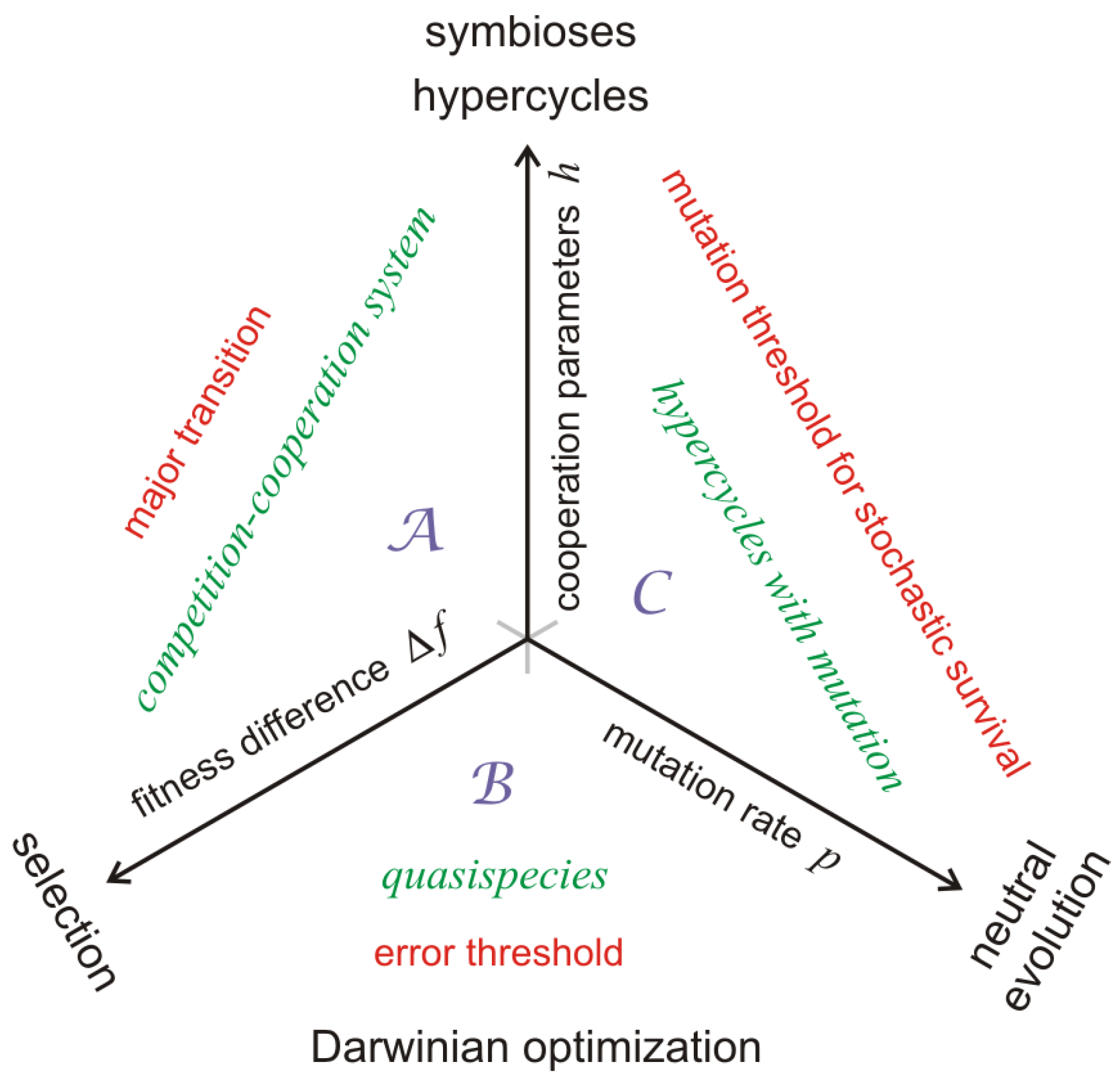
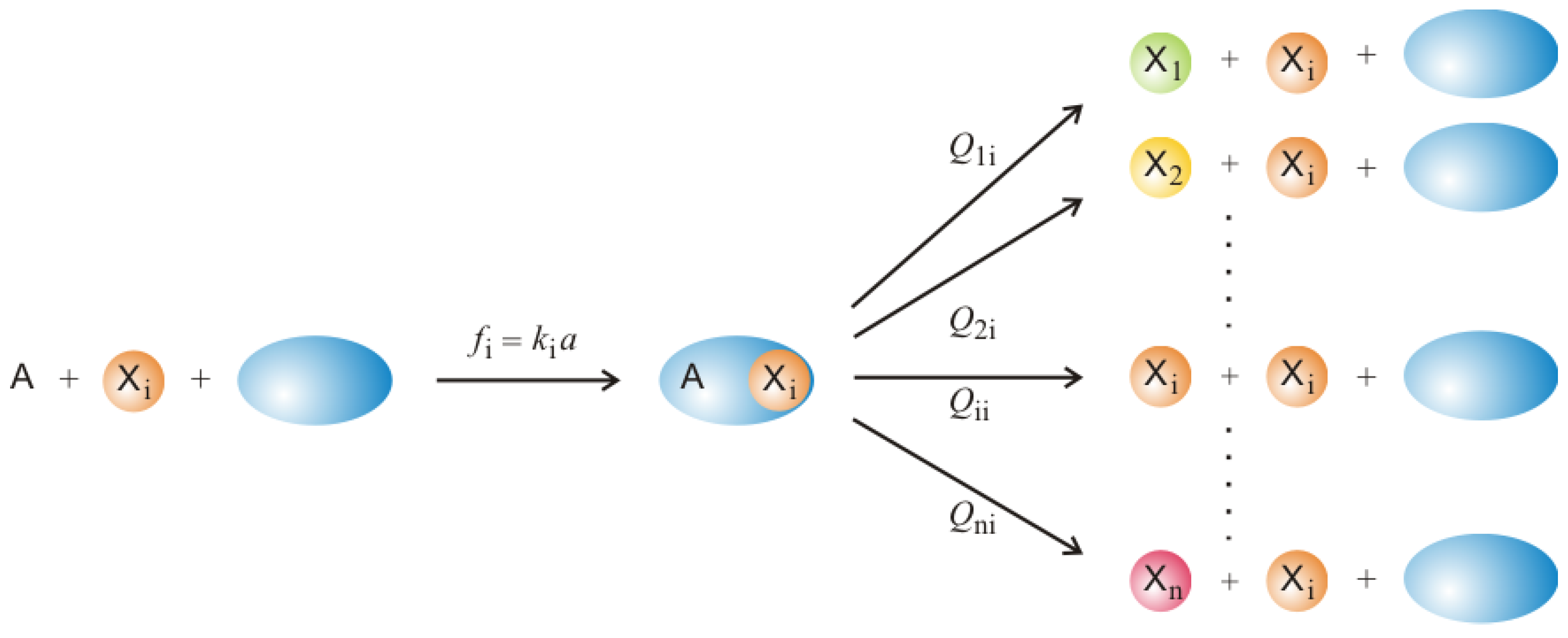
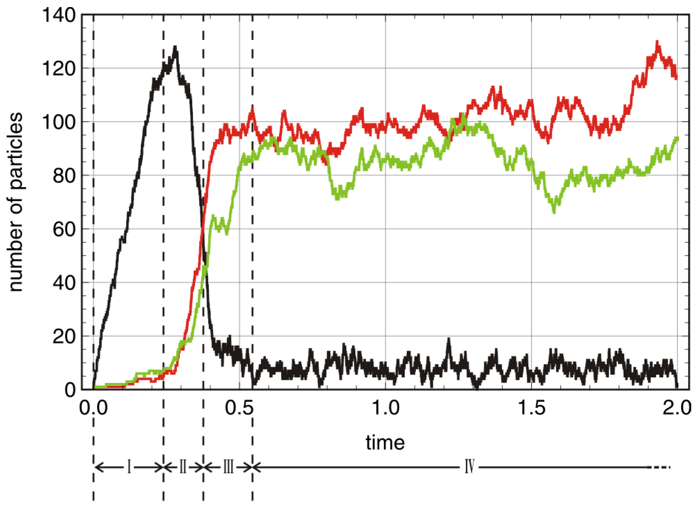
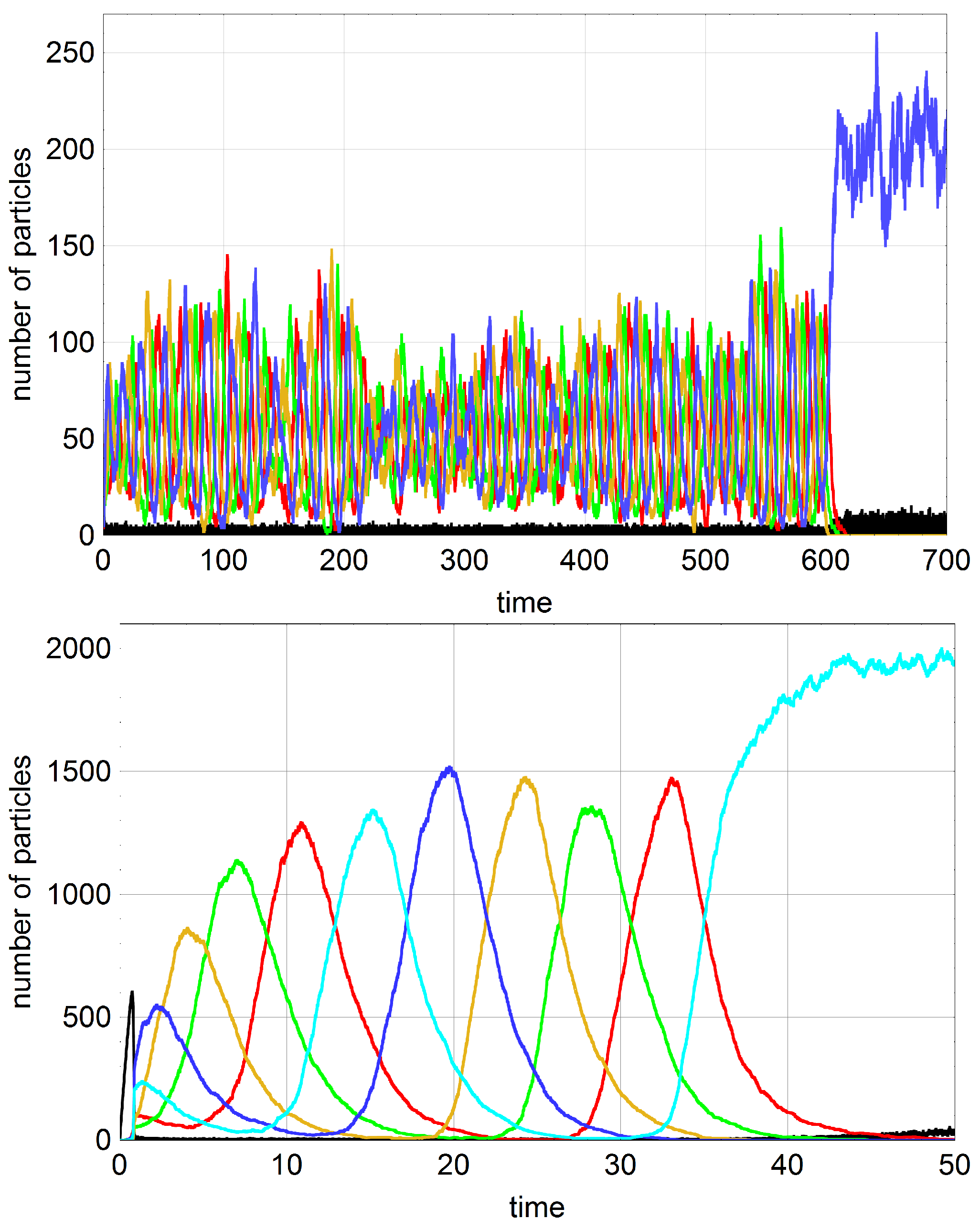
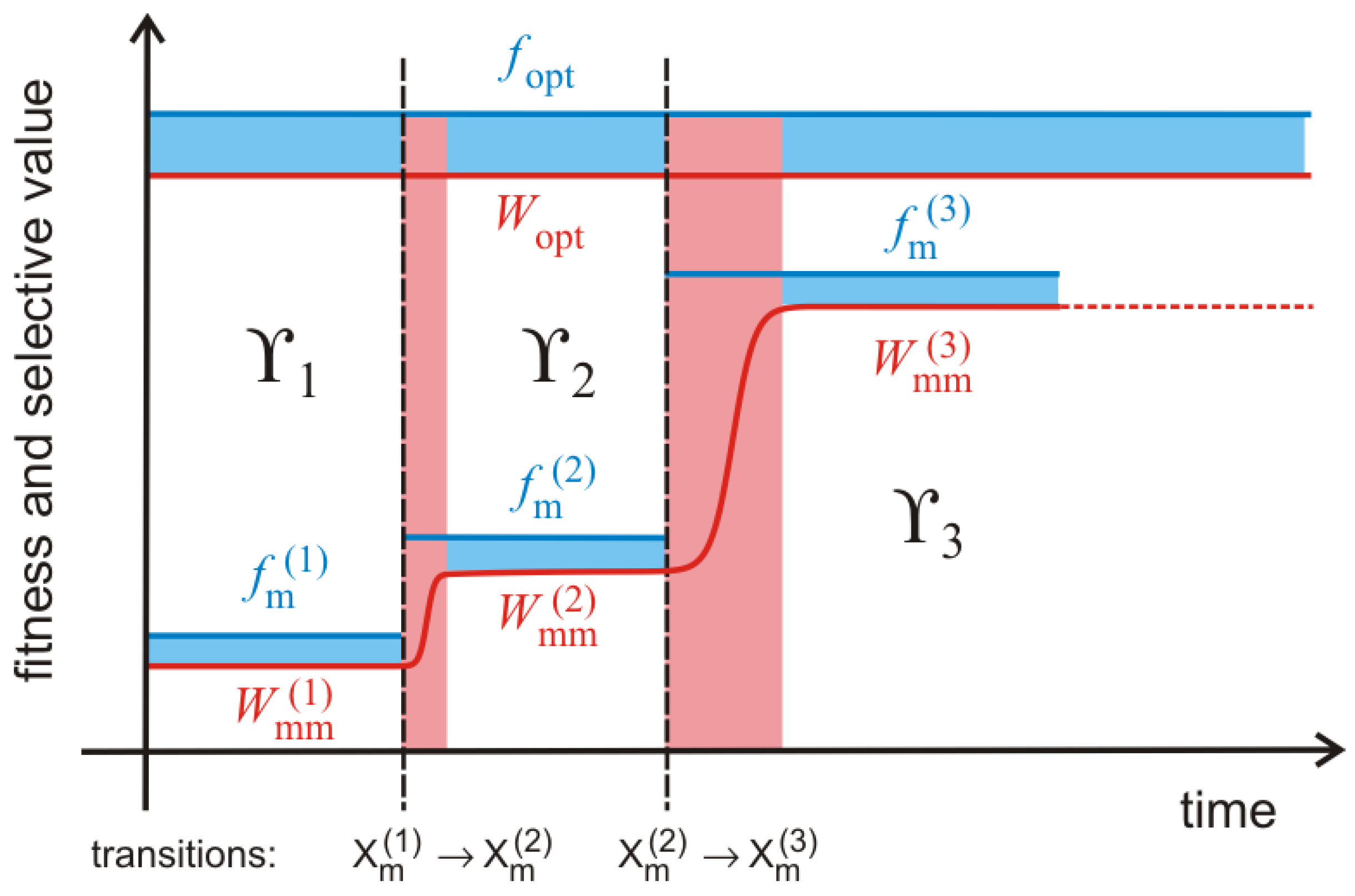
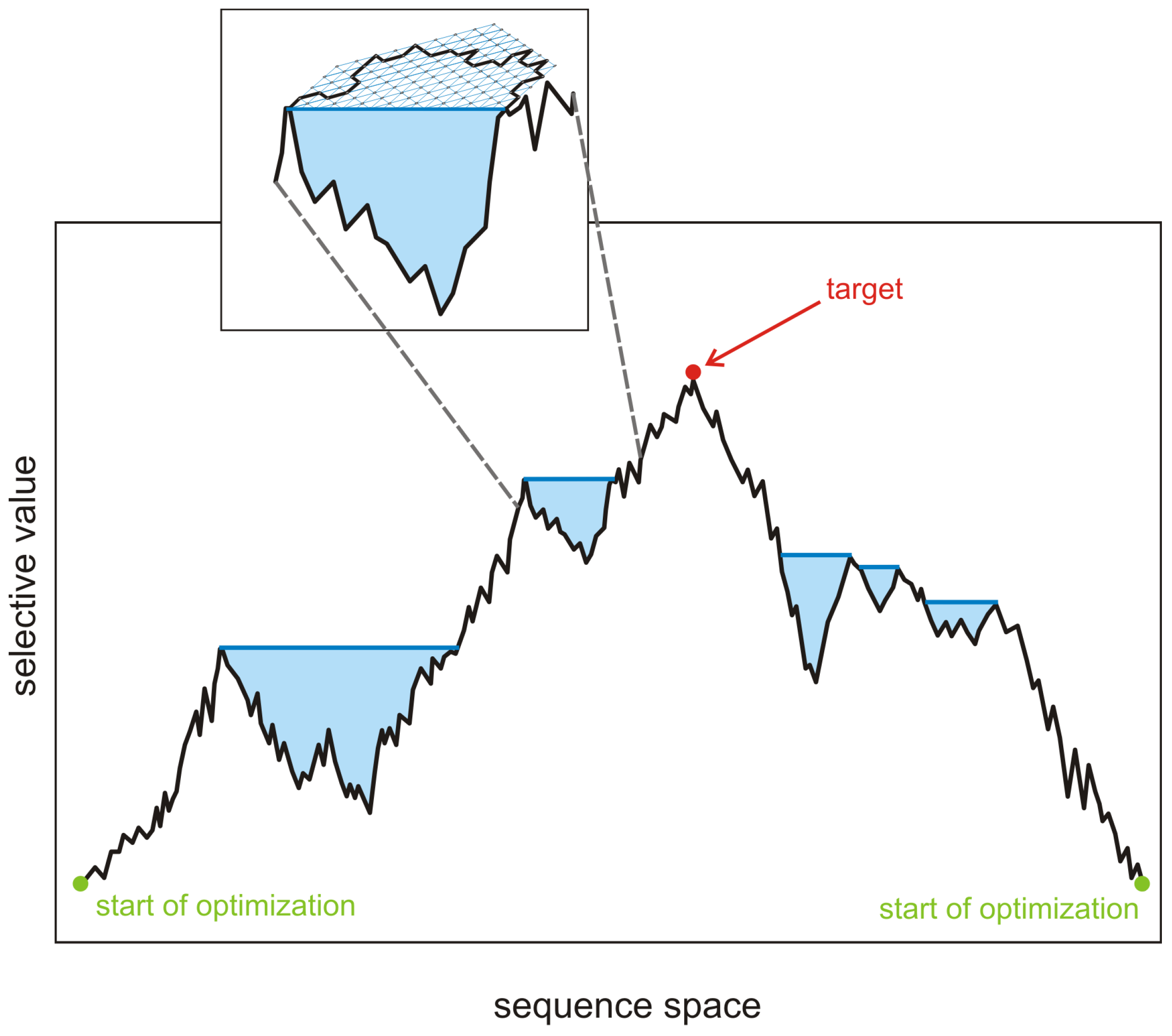
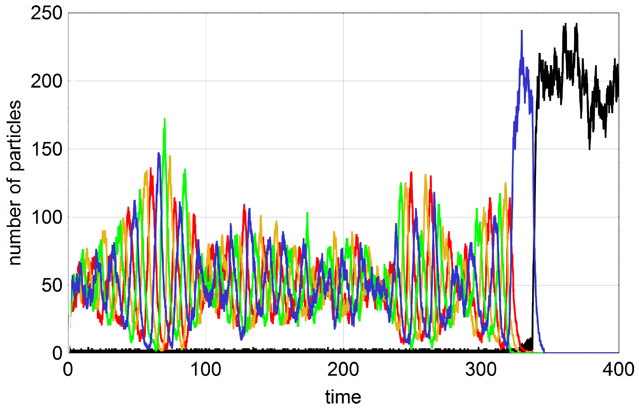
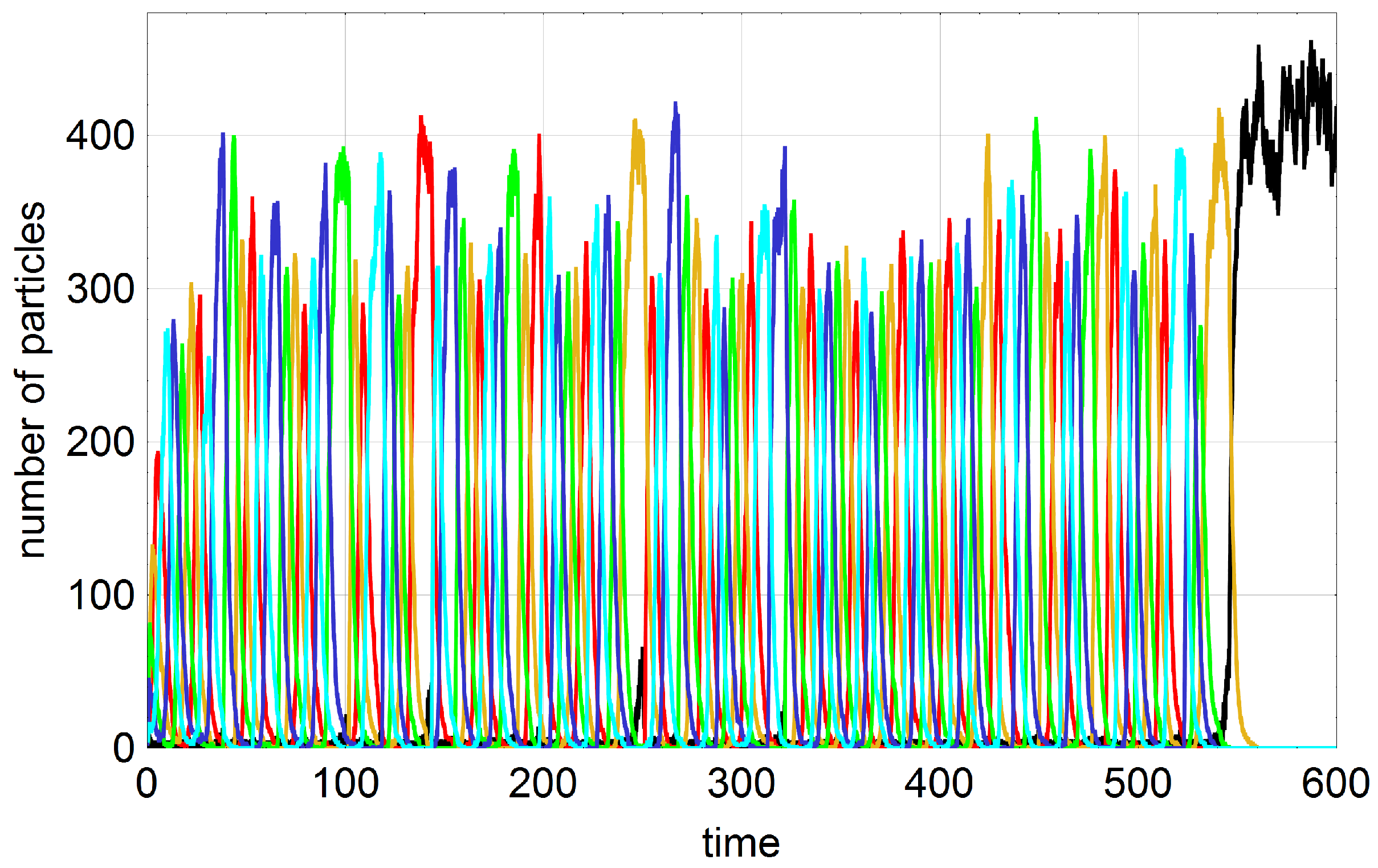
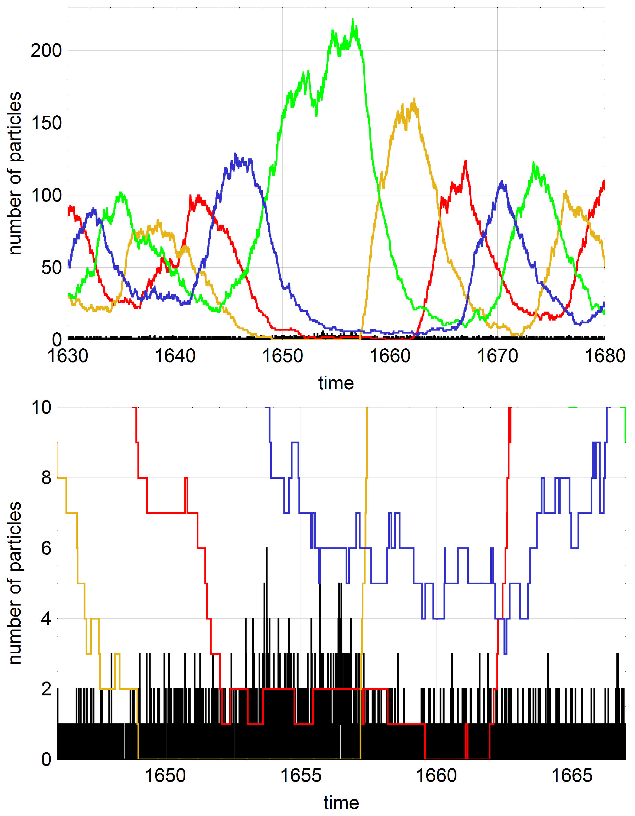
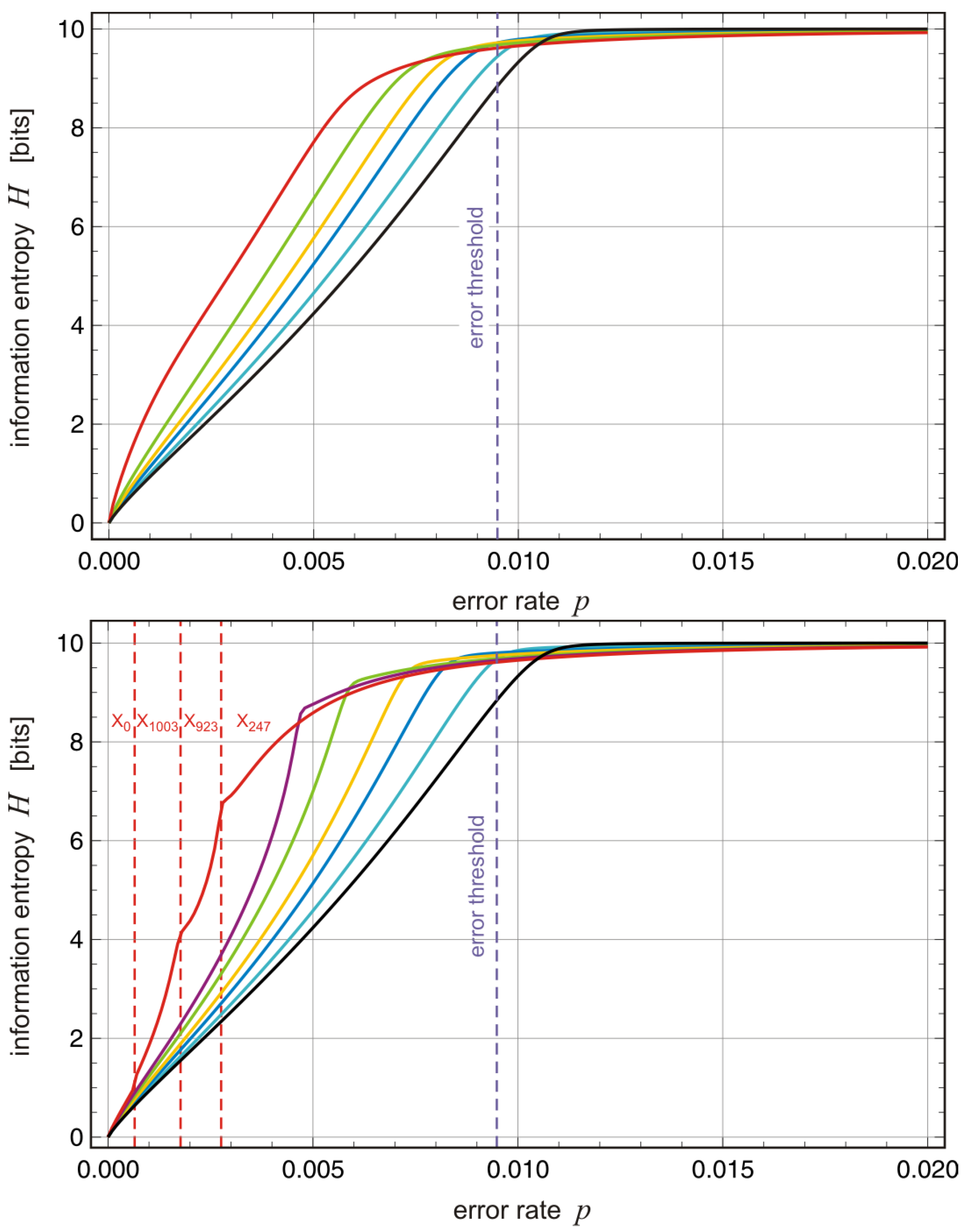
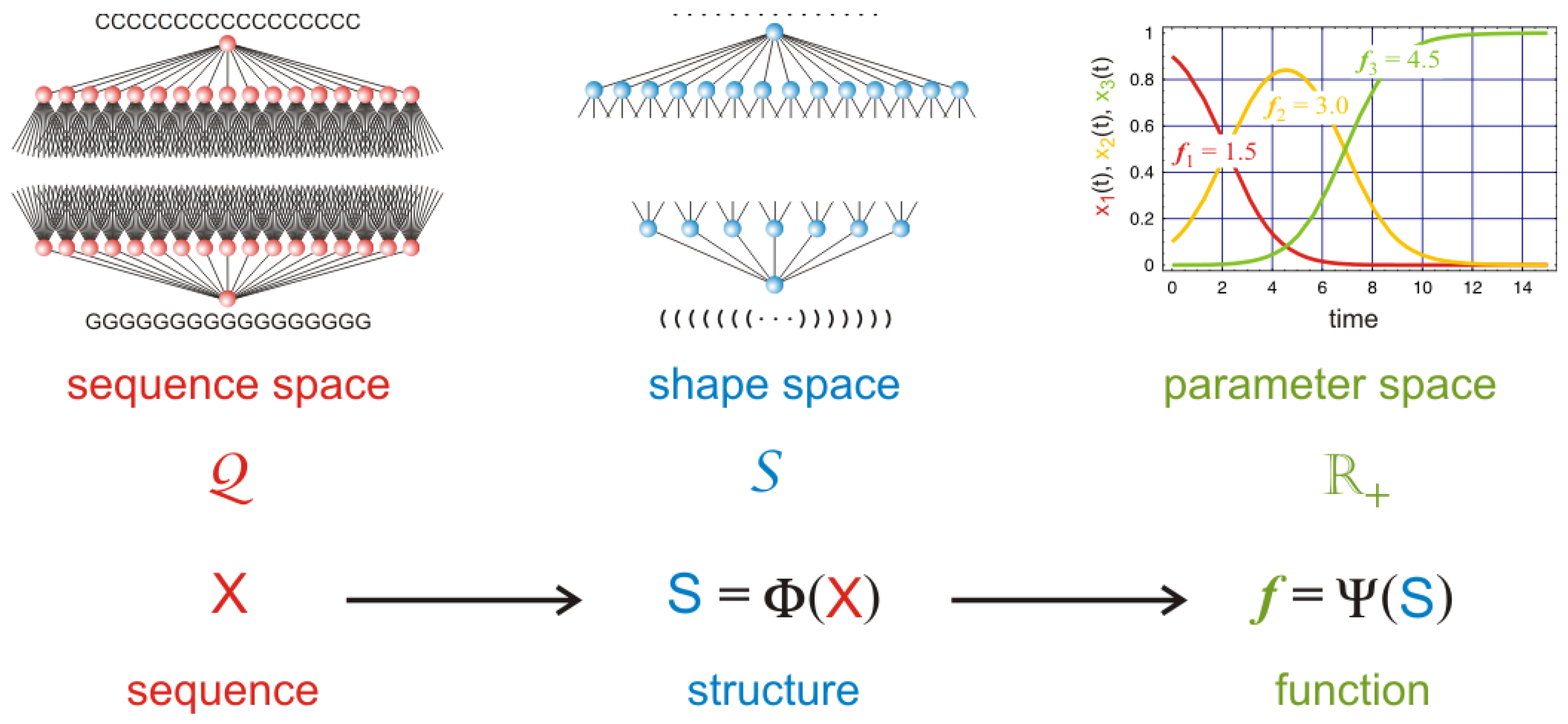
Table 1.
Asymptotically stable stationary states of Equation (4) with [9]. The three stationary states are ordered with respect to increasing -values of their asymptotically stable regimes. Validity of the relations and between rate parameters was assumed. For the cooperative state stationary concentration of A is obtained as the root with the negative sign of the quadratic Equation (5) with two combinations of the rate parameters, and . The existence of the cooperative state requires in addition a sufficiently small flow rate: .
| Name | Symbol | Stationary Values | Stability Range | ||
|---|---|---|---|---|---|
| extinction | 0 | 0 | |||
| selection | 0 | ||||
| cooperation | α | ||||
Table 2.
Asymptotically stable stationary states of Equation (4) with [9]. The four stationary states are ordered with respect to increasing -values of their asymptotically stable regime. The relations and between the rate parameters were assumed. For the cooperative state the stationary concentration of A is obtained as one root of a quadratic Equation (5) with two combinations of the rate parameters, and . The existence of the cooperative state requires a sufficiently small flow rate: .
| Name | Symbol | Stationary Values | Stability Range | |||
|---|---|---|---|---|---|---|
| extinction | 0 | 0 | 0 | |||
| selection | 0 | 0 | ||||
| exclusion | 0 | |||||
| cooperation | α | |||||
Table 3.
Probabilities to reach states in the cooperative regime with and different initial conditions. The table provides counts of approach towards the four final states: extinction , selection of in , selection of in , or cooperation . The given values are sample means and unbiased standard deviations calculated from ten packages, each of them containing 10,000 trajectories computed with identical parameters and initial conditions, and differing only in the sequence of random events determined by the seeds of the pseudorandom number generator (Extended CA, Mathematica). Choice of parameters: [Mt], [Mt], [Mt], [Mt], , [V t]. Initial conditions: , and see table.
| Initial Values | Counted Numbers of States in Final Outcomes | ||||
|---|---|---|---|---|---|
| 1 | 1 | ||||
| 2 | 1 | ||||
| 1 | 2 | ||||
| 3 | 1 | ||||
| 1 | 3 | ||||
| 2 | 2 | ||||
| 3 | 3 | 0 | |||
| 4 | 4 | 0 | |||
| 5 | 5 | 0 | |||
Table 4.
Extinction times of cooperative populations with as a function of the mutation rate parameter . A limit for recording trajectories is set with steps. Choice of parameters and initial conditions: , [Vt], [Mt], , . Pseudorandom number generator: Extended CA (Mathematica 10).
| : Mutation Rate Parameter p | |||||||
|---|---|---|---|---|---|---|---|
| Seed | 0.0 | 0.001 | 0.002 | 0.0025 | 0.003 | 0.004 | 0.005 |
| 491d | 1212.4 | 654.5 | 313.0 | 636.0 | >3000 | >3000 | 1939.4 |
| 919 | 292.4 | 1069.7 | 1764.8 | 2920.1 | >3000 | >3000 | >3000 |
| 521 | 25.3 | 25.3 | 23.8 | 30.0 | 27.1 | 43.7 | 28.4 |
| 877 | 1920.5 | 367.1 | 1863.8 | 308.4 | >3000 | 1940.9 | 1146.9 |
| 233 | 85.3 | 71.2 | 1532.6 | >3000 | 1617.9 | 84.9 | 2398.7.4 |
| 373 | 1017.7 | 482.2 | 1668.3 | 525.1 | 1146.2 | 1231.5 | >3000 |
| 089 | 319.4 | 338.5 | 75.3 | 82.4 | 81.0 | 1239.8 | 81.0 |
| 773 | 161.2 | 411.2 | 361.8 | 2297.2 | >3000 | >3000 | >3000 |
| 131 | 936.2 | 1059.8 | 78.0 | 1362.4 | 1742.9 | >3000 | >3000 |
| 631 | 135.0 | 60.4 | 670.3 | >3000 | 87.8 | 884.4 | 978.4 |
| mean | 600 | 500 | 800 | - | - | - | - |
Table 5.
Extinction times of cooperative populations with as a function of the mutation rate parameter . A limit for recording trajectories is set with steps. Choice of parameters and initial conditions: , [Vt], [Mt], , . Pseudorandom number generator: Extended CA (Mathematica 10).
| : Mutation Rate Parameter p | ||||||
|---|---|---|---|---|---|---|
| Seed | 0.0 | 0.0005 | 0.0010 | 0.0015 | 0.0020 | 0.0025 |
| 491 | 36.1 | 31.3 | 56.2 | 118.9 | 48.1 | 652.9 |
| 919 | 52.9 | 42.9 | 81.6 | 229.9 | 546.9 | >1650 |
| 521 | 39.0 | 80.9 | 96.2 | 116.1 | 366.3 | 210.0 |
| 877 | 34.4 | 40.6 | 70.2 | 310.6 | 1611.6 | 1541.6 |
| 233 | 23.8 | 85.2 | 34.6 | 310.2 | 90.9 | >1650 |
| 373 | 41.2 | 45.5 | 105.8 | 680.4 | 50.1 | >1650 |
| 089 | 29.5 | 28.3 | 73.3 | 97.7 | 831.3 | >1650 |
| 773 | 50.7 | 73.8 | 85.7 | 485.2 | 682.3 | >1650 |
| 131 | 21.5 | 21.5 | 80.0 | 104.0 | 953.1 | >1650 |
| 631 | 33.0 | 78.6 | 68.9 | 265.7 | 298.7 | 248.0 |
| mean | 37 | 53 | 75 | 272 | 548 | - |
© 2016 by the author; licensee MDPI, Basel, Switzerland. This article is an open access article distributed under the terms and conditions of the Creative Commons Attribution (CC-BY) license (http://creativecommons.org/licenses/by/4.0/).
Share and Cite
MDPI and ACS Style
Schuster, P. Increase in Complexity and Information through Molecular Evolution. Entropy 2016, 18, 397. https://0-doi-org.brum.beds.ac.uk/10.3390/e18110397
AMA Style
Schuster P. Increase in Complexity and Information through Molecular Evolution. Entropy. 2016; 18(11):397. https://0-doi-org.brum.beds.ac.uk/10.3390/e18110397
Chicago/Turabian StyleSchuster, Peter. 2016. "Increase in Complexity and Information through Molecular Evolution" Entropy 18, no. 11: 397. https://0-doi-org.brum.beds.ac.uk/10.3390/e18110397
Note that from the first issue of 2016, this journal uses article numbers instead of page numbers. See further details here.