Feature Selection of Power Quality Disturbance Signals with an Entropy-Importance-Based Random Forest

Abstract

Power quality signal feature selection is an effective method to improve the accuracy and efficiency of power quality (PQ) disturbance classification. In this paper, an entropy-importance (EnI)-based random forest (RF) model for PQ feature selection and disturbance classification is proposed. Firstly, 35 kinds of signal features extracted from S-transform (ST) with random noise are used as the original input feature vector of RF classifier to recognize 15 kinds of PQ signals with six kinds of complex disturbance. During the RF training process, the classification ability of different features is quantified by EnI. Secondly, without considering the features with zero EnI, the optimal perturbation feature subset is obtained by applying the sequential forward search (SFS) method which considers the classification accuracy and feature dimension. Then, the reconstructed RF classifier is applied to identify disturbances. According to the simulation results, the classification accuracy is higher than that of other classifiers, and the feature selection effect of the new approach is better than SFS and sequential backward search (SBS) without EnI. With the same feature subset, the new method can maintain a classification accuracy above 99.7% under the condition of 30 dB or above, and the accuracy under 20 dB is 96.8%.

1. Introduction

Power quality (PQ) is the main control target of the smart grid, and PQ signal recognition is the foundation of PQ problem management [1]. With the wide access of distributed generators (DGs) to the power system, many renewable power sources with random output characteristics, such as distributed solar energy and wind power, have a negative impact on the PQ of the power system [2]. Then, it is necessary to carry out in-depth monitoring and analysis of the PQ in all points accessed by DGs [3]. Therefore, the massive PQ data collected from a large number of monitors represents a higher real-time requirement for any PQ signal classification system [4].

Features extracted from the time-frequency analysis (TFA) results are always used as the input of the classifier for PQ disturbances identification. Previous studies have carried out a lot of in-depth research on TFA of PQ signals, including Hilbert–Huang transform (HHT) [5,6], S-transform (ST) [7,8,9] and discrete wavelet transform (DWT) [10,11,12]. In the current research results, the environmental noise is the main factor which affects the PQ classification accuracy, especially in the distribution network. ST has been proved to have good anti-noise abilities among all the TFA methods [7,8,9]. Feature extraction of PQ signals using ST and its improved form has been paid more and more attention. Nevertheless, existing methods extract a large number of features according to the ST results, but the ability of the features to identify the disturbances lacks effective analysis. The high feature vector dimension increases the complexity, reduces the classification efficiency and accuracy of PQ disturbances classifier. Moreover, the feature vectors used in different research are diverse. This will enhance the difficulties of constructing a unified PQ signal classifier. For the sake of simplifying the classifier and enhancing the classification efficiency, it is essential to add the feature selection step in the PQ disturbances recognition process.

In past studies, feature selection was either in accordance with the filter method based on the features’ statistical characteristics, which made it difficult to analyze the classification ability of the feature combination [13,14], or used the wrapper method combined with the particle swarm optimization [15], genetic algorithm [16], rough set theory [17] or other intelligent algorithms, then according to the classification results chose the optimal or sub-optimal feature subset, but the efficiency of the search algorithm is unsatisfactory. Meanwhile, existing feature selection methods have to select different feature subsets under different noise conditions, and this limits the application possibilities of feature selection methods in practical engineering.

From the perspective of classifier design steps, neural network (NN) [18,19,20], support vector machine (SVM) [21,22,23], fuzzy rule (FR) [24], decision tree (DT) [25,26,27] and extreme learning machine (ELM) [28] are commonly applied to the classification of PQ signals, and all achieve good results. However, the NN and SVM have to set more parameters. This will lead to the difficulty of designing the classifier and makes it easier to fall into over-fitting. FR and DT have simple structures with higher classification accuracy and efficiency than NN and SVM [24,25,26,27], but it is difficult to choose the optimization threshold of the classification threshold of FR and DT.

Random forest (RF) is an excellent classifier model with advantages such as good anti-noise performance, less parameters and less influence of the over-fitting problem. Moreover, RF has better generalization ability than DT [29]. In the verification of multiple public data sets, the classification accuracy of RF is the highest among all methods [30]. What’s more, RF is an effective method for the integration of feature selection. During the training process, classification ability of each feature can be obtained according to the training results of RF’s every node. Then the optimal feature subset can be selected out on the basis of this. The analysis process of feature selection method based on RF is parallel to the filter method. At the same time, RF can adjust the optimum feature subset based on the classification accuracy on the new testing sets of different feature subsets as the wrapper approach, but more efficient. The feature selection process of RF takes both the statistical conclusion of the characteristics and the classification results of the classifier into consideration. It combines the virtues of the filter method and wrapper method. Therefore, RF has good applicability for feature selection.

For the sake of finding the optimizing feature subset and increasing the classification accuracy of PQ disturbances, a new method for PQ disturbances feature selection and classification using a entropy-importance (EnI)-based RF is proposed in this paper. Firstly, 15 kinds of PQ signals including six kinds of complex disturbance are simulated by a mathematical model. Then, the simulation signals are processed by ST to extract 35 kinds of commonly used features for PQ classification. Secondly, a RF classifier used for recognizing PQ signals is constructed with the original feature subset as the input vector. According to EnI score of features obtained from the RF training process, classification ability of each feature can be sorted to construct the optimal subset. Features with zero EnI score will not be selected. On this basis, a sequential forward search (SFS) strategy is adopted to determine the optimal feature subset and RF based classifier with optimal feature subset is reconstructed. Finally, the optimized RF classifier is used to recognize PQ signals. Simulation experiment results show that the new method is valid.

The remainder of the paper is designed as follows: Section 2 presents the basic theory and the classification process of RF. In Section 3, it describes the details of the new approach including the segmentation of non-leaf node, the calculation of EnI of each feature, and the feature selection strategy based on EnI. Then, the results of different simulation experiments are shown and discussed in Section 4. Finally, Section 5 presents the conclusions of this paper.

2. Classification by Random Forest

RF combines DT with ensemble learning to form a new kind of tree classifier:

$$\{f(x,{\delta }_k),k=1,\cdots \}$$

(1)

where $f(x,{\delta }_k)$ is a meta classifier, and it is a tree construct classifier that can be formed by several algorithms; x is the input vector; ${\delta }_k$ is a random vector, independent with each other but sharing the same distribution, and it determines the growth of a single decision tree. RF generates a random feature subset in each non-leaf node of DT, and chooses the feature contained in this subset with the best classification results to split this node. Finally, RF summarizes the classification results of different DTs to achieve the optimal classification result. Compared to DT, RF overcomes the weakness of generalization ability, and improves the classification accuracy without significantly increasing the amount of computing.

2.1. RF Classification Capability Analysis

Generalization error is an important index to measure the extrapolation ability of the classifier. The classification ability of RF can be measured by analyzing its generalization error [29]. Given a classifier set $F(x)=\left\{f_1(x),f_2(x),\dots ,f_k(x)\right\}$, and the training set of each classifier is obtained from the original data set $(X,Y)$ by random sampling. The margin function is:

$$marg(X,Y)=av{e}_{k}IN(f_k(X)=Y)-\underset{j\ne Y}{\max } av{e}_{k}IN(f_k(X)=j)$$

(2)

here, $IN(\cdot )$ is an indicator function, $av{e}_k(\cdot )$ is average value, Y is the correct classification of the vector, j is the incorrect classification of the vector.

The margin function measures the degree of the average correct classification number of classifiers exceeds the average number vote for any other class. The larger the margin function, the better the classification performance. The generalization error is calculated by:

$$P{E}^{*}=P_{X,Y}(marg(X,Y)<0)$$

(3)

here, the subscript X, Y represent the definition of space.

In RF, $f_k(X)=f(X,{\delta }_k)$. With the growth of tree number of RF, it can be known from the Strong Law of Large Numbers and the tree structure that:

$$\underset{k\to \infty }{\lim }P{E}^{*}=P_{X,Y}(P_{\delta }(f(X,\delta )=y)-\underset{j\ne Y}{\max }{P}_{\delta }(f(X,\delta )=j)<0)$$

(4)

where $P_{\delta }(f(X,\delta )=y)$ represents the probability of the classification results as the right class and $\underset{j\ne Y}{\max }{P}_{\delta }(f(X,\delta )=j)$ represents the maximum probability of the classification results as any other class. Equation (4) denotes that $P{E}^{*}$ tend to a constant as the tree number increases, so RF is not easy to produce over-fitting problem. The margin function of RF is given as:

$$marr(X,Y)=P_{\delta }(f_k(X,\delta )=Y)-\underset{j\ne Y}{\max }{P}_{\delta }(f(X,\delta )=j)$$

(5)

Then, the strength of $\{f(x,{\delta }_k)\}$ is the mathematical expectation of $marr(X,Y)$:

$$str=E_{X,Y}marr(X,Y)$$

(6)

Assuming $str\ge 0$, according to Chebychev’s inequality, there is:

$$P{E}^{*}\le \frac{\mathrm{var}(marr)}{st{r}^2}$$

(7)

where $\mathrm{var}(marr)$ is the variance of $marr(X,Y)$. In order to make more detailed description about $\mathrm{var}(marr)$, let:

$$\widehat{j}(X,Y)=\arg \underset{j\ne Y}{\max }{P}_{\delta }(f(X,\delta )=j)$$

(8)

Then:

$$\begin{array}{l}marr(X,Y)=P_{\delta }(f(X,\delta )=Y)-P_{\delta }(f(X,\delta )=\widehat{j}(X,Y))\\ \hspace{1em}\hspace{1em}\hspace{1em}=E_{\delta }[IN(f(X,\delta )=Y)-IN(f(X,\delta )=\widehat{j}(X,Y))]\end{array}$$

(9)

The margin function of meta classifier is defined as:

$$rmarg(\delta ,X,Y)=IN(f(X,\delta )=Y)-IN(f(X,\delta )=\widehat{j}(X,Y))$$

(10)

Therefore, $marr(X,Y)$ is the expectation of $rmarg(\delta ,X,Y)$ in regard to $\delta$. No matter what function h is, there is:

$$[E_{\delta }h{(\delta )}^2]=E_{\delta ,{\delta }^{\prime }}h(\delta )h({\delta }^{\prime })$$

(11)

here $\delta$ and ${\delta }^{\prime }$ are independent with each other and share the same distribution, so:

$$marr{(X,Y)}^2=E_{\delta ,{\delta }^{\prime }}rmarg(\delta ,X,Y)rmarg({\delta }^{\prime },X,Y)$$

(12)

According to Equation (12), it can be obtained:

$$\begin{array}{l}\mathrm{var}(marr)=E_{\delta ,{\delta }^{\prime }}({\mathrm{cov}}_{X,Y}rmarg(\delta ,X,Y)rmarg({\delta }^{\prime },X,Y))\\ \hspace{1em}\hspace{1em}\hspace{1em}=E_{\delta ,{\delta }^{\prime }}(\rho (\delta ,{\delta }^{\prime })sd(\delta )sd({\delta }^{\prime }))\end{array}$$

(13)

when $\delta$ and ${\delta }^{\prime }$ are holding fixed, $\rho (\delta ,{\delta }^{\prime })$ is the correlation between $rmarg(\delta ,X,Y)$ and $rmarg({\delta }^{\prime },X,Y)$; $sd(\delta )$ and $sd({\delta }^{\prime })$ are the standard deviation of $rmarg(\delta ,X,Y)$ and $rmarg({\delta }^{\prime },X,Y)$ respectively. Then the conditional functional of $\mathrm{var}(marr)$ need to be met are obtained:

$$\{\begin{array}{c}\mathrm{var}(marr)=\overline{\rho }{(E_{\delta }sd(\delta ))}^2\\ \mathrm{var}(marr)\le \overline{\rho }(E_{\delta }\mathrm{var}(\delta ))\end{array}$$

(14)

where $\overline{\rho }$ is the mean correlation value. Then we have the function as follows:

$$\{\begin{array}{l}{E}_{\delta }\mathrm{var}(\delta )\le E_{\delta }{(E_{X,Y}rmarg(\delta ,X,Y))}^2-st{r}^2\\ E_{\delta }\mathrm{var}(\delta )\le 1-st{r}^2\end{array}$$

(15)

Put (7), (14), and (15) together yields the function as:

$$P{E}^{*}\le \frac{\overline{\rho }(1-s^2)}{s^2}$$

(16)

When increasing the strength of the individual classifiers or decreasing the correlation between classifiers, the generalization error tends to a loose upper bound, so RF has good generalization ability. Meanwhile, with the increase of forest size, so it is not easy for RF to fall into over-fitting.

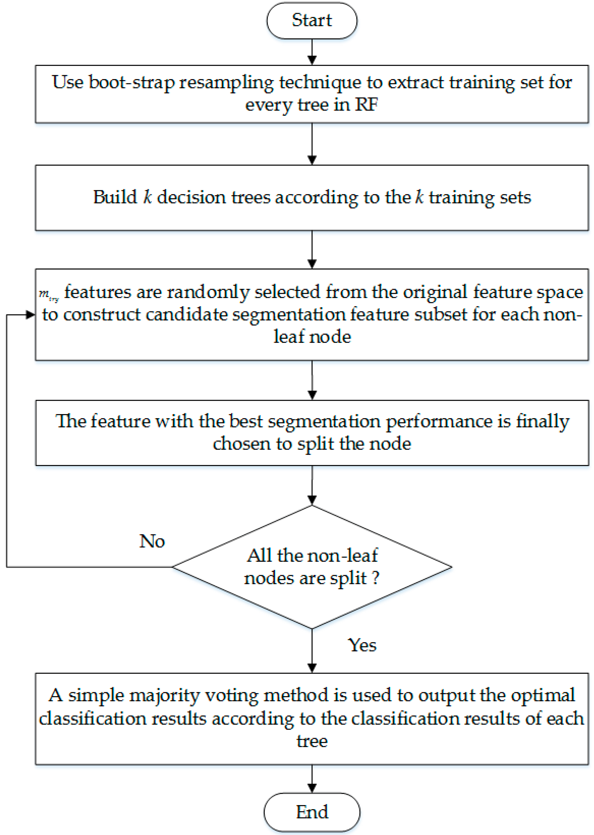
2.2. The Classification Process of RF

RF has a simple structure, good generalization ability and anti-noise performance [31]. Compared to other classifiers, the time complexity of RF is lower, and RF can achieve higher classification accuracy. Thus, RF can meet the application needs of massive PQ signal classification. The steps for the classification of RF are described as follows:

• The boot-strap resampling technique is used to extract the training set for every tree in RF, and the size of training set is equal to the original data set. Samples that haven’t been extracted are composed of out-of-bag data set. K training sets and out-of-bag data sets will be extracted by repeating the above process k times.
• K decision trees are built according to the k training sets to construct a RF.
• During the training process, $m_{try}$ features are randomly selected from the original feature space to construct candidate segmentation feature subset for each non-leaf node. Most studies let $m_{try}=\sqrt{t}$, where t is the number of original features.
• Each feature in the candidate segmentation feature subset is used to split the node, and the feature with the best segmentation performance is finally chosen as the segmentation feature of the node.
• Repeat step 3 and step 4 until all non-leaf nodes segmented, then the training process is over.
• When using RF to classify PQ signals, a simple majority voting method is used to output the optimal classification results according to the classification results of each classifier.

The steps of the classification process are presented in Figure 1.

Figure 1. Flow diagram of the RF based classification.

Figure 1. Flow diagram of the RF based classification.

3. Construction of RF and Feature Selection of PQ Signals Based on EnI

3.1. EnI Calculation and Node Segmentation

When using a feature to split the non-leaf node of a decision tree, there are two kinds of indicators to measure the segmentation effect: information gain [32] and Gini index [33]. Information gain is calculated from entropy like mutual information, which is always used for feature selection [34]. Applying these two indicators to RF, the EnI and Gini-importance (GiI) of each feature can be obtained, respectively. During the training process, the EnI method can set the importance of features that have no or little contribution to the classification to zero. Based on this, the EnI method can greatly reduce the feature selection workload when compared to the existing GiI method. The features with the zero EnI do not have to be considered. Therefore, EnI based feature selection method is able to meet the actual needs of mass PQ signal classification.

Entropy is a quantitative measurement method of data carrying information. The more uniform the data distribution, the greater its entropy value. Assuming the node, which is going to be split, is composed of a set S, and S contains s samples and n class. The entropy of the node is given as:

$$H(s_1,s_2,\cdots ,s_n)=-{\displaystyle \sum _{k=1}^n{P}_k{\log }_2(P_k)}$$

(17)

where, $s_k$ is sample number in class k $(k=1,2,\cdots ,n)$; $P_k=s_k/s$ expresses the possibility that a sample belongs to class i. When S contains only one class, its entropy is zero; when all the classes in S are distributed evenly, the maximum value of the information entropy is taken.

Assuming when RF uses a feature A to split the node, S can be divided into m subsets $S_j$, where $j=1,2,\cdots ,m$. Then the entropy of A splitting the node is defined as:

$$E_{split}={\displaystyle {\sum }_{j=1}^m\frac{s_{1j}+\cdots +s_{nj}}{s}}\cdot H(s_{1j},\cdots ,s_{nj})$$

(18)

where, $s_{ij}$ is the number of sample of class i in subset $S_j$. According to Equations (17) and (18), the information gain of A splitting the node can be obtained as:

$$Gain(A)=H(s_1,\cdots ,s_n)-E_{split}$$

(19)

The information gain of each feature in the candidate segmentation feature subset can be calculated according to Equations (17)– (19). According to the new feature selection method, the feature which has the highest $Gain$ value is chosen as the segmentation feature of this node, and the information gain of other features (all features in original feature space except feature A) is set to zero:

$$Gain(A)=\{\begin{array}{l}Gain(A)\text{ feature A has the highest information gain}\\ \hspace{1em}0\text{\hspace{1em}\hspace{1em}\hspace{1em}\hspace{1em}\hspace{1em}\hspace{1em}else}\end{array}$$

(20)

After the completion of the RF, the EnI of a feature can be obtained by linear superposition of its all information gain values:

$$EnI(A)={\displaystyle \sum _{i=1}^{n}Gain(A)}$$

(21)

where $n$ represents the all non-leaf node number in RF.

Finally, the importance of each feature can be analyzed by sorting all features in descending order according to their EnI. The feature with higher EnI will be used to construct the optimal feature set.

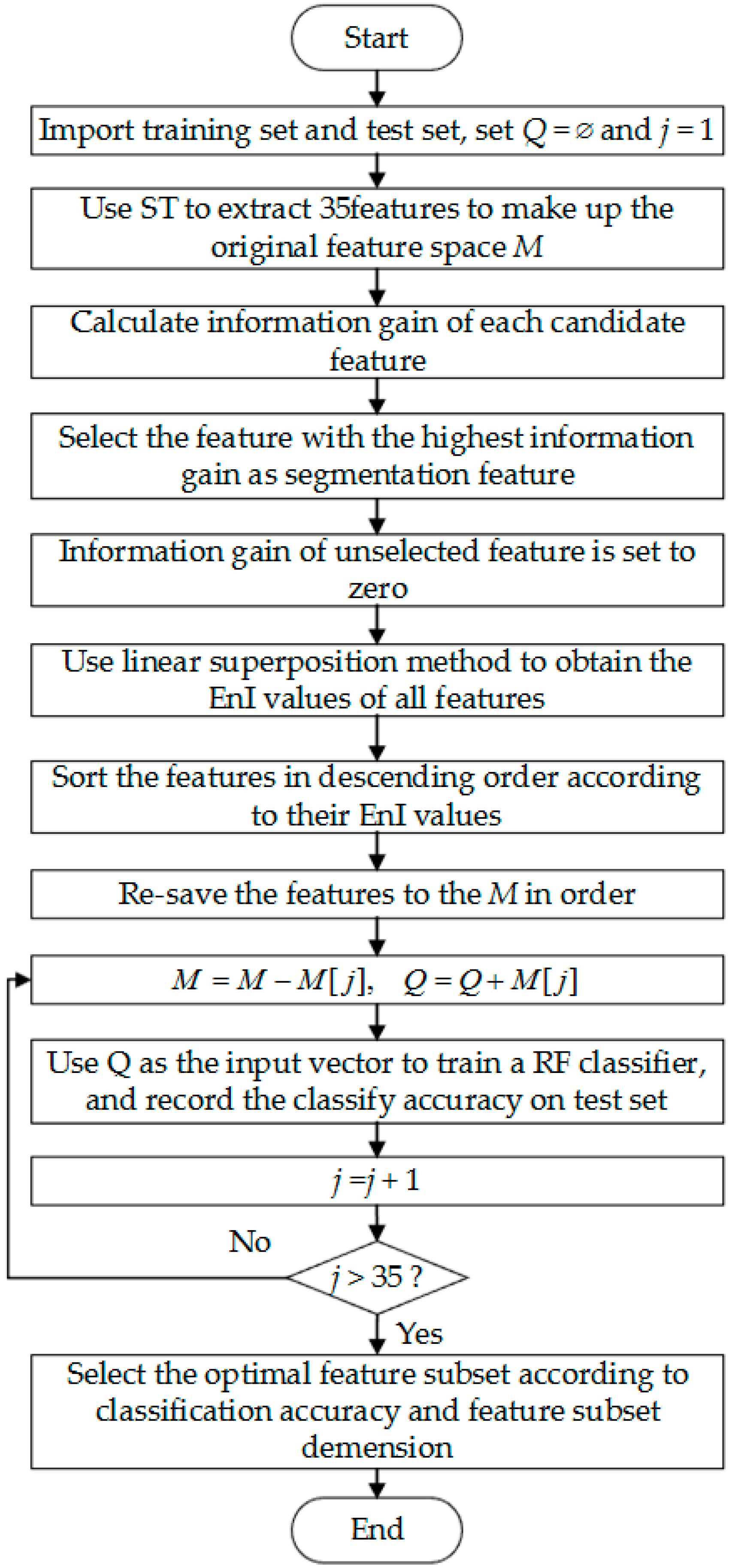
3.2. Forward Search Strategy of PQ Feature Selection Based on EnI

In this paper, the SFS algorithm [35] based on EnI is proposed for PQ feature selection. Firstly, according to the descending sort order of the features based on their important degree, the feature is added to the selected feature subset Q one by one. Subset Q is used as the input vector of RF to retrain a classifier when a new feature is added, and the classification accuracy need to be recorded. Then, the process is repeated until all features are added into Q. Finally, the optimal feature subset is determined by taking both classification accuracy and the dimension of selected feature subset into consideration. The process of feature selection needs to be performed only one time to train the RF classifier. The flow diagram of the new method is shown as Figure 2.

Figure 2. Flow diagram of the new feature selection method.

Figure 2. Flow diagram of the new feature selection method.

4. Experimental Results and Analysis

Through the simulation contrast experiment, the new method is analyzed and validated in aspects of feature selection methods, classifier performance, and signal processing methods.

4.1. Feature Extraction of PQ Signals

Referring to [13,15], 15 kinds of PQ signals are generated by simulation, including normal (C0), sag (C1), swell (C2), interruption (C3), flicker (C4), transient (C5), harmonic (C6), notch (C7), spike (C8), harmonic with sag (C9), harmonic with swell (C10), harmonic with flicker (C11), sag with transient (C12), swell with transient (C13) and flicker with transient (C14). The sampling frequency is 3.2 kHz, and the fundamental frequency is 50 Hz. For the sake of improving the capability of features extracted from ST, according to literature [25], the different values of the window width factor are given in different frequency domain. The original features extracted from ST modular matrix (STMM) are described as follow [13]:

• Feature 1 (F1): the maximum value of the maximum amplitude of each column in STMM (A_max).
• Feature 2 (F2): the minimum value of the maximum amplitude of each column in STMM (A_min).
• Feature 3 (F3): the mean value of the maximum amplitude of each column in STMM (Mean).
• Feature 4 (F4): the standard deviation (STD) of the maximum amplitude of each column in STMM (STD).
• Feature 5 (F5): the amplitude factor ($A_f$) of the maximum amplitude of each column in STMM, defined as $A_f=\frac{A_{\max }+A_{\min }-1}{2}$ in the range $0<A_f<1$.
• Feature 6 (F6): the STD of the maximum amplitude in the high frequency area above 100 Hz.
• Feature 7 (F7): the maximum value of the maximum amplitude in the high frequency area above 100 Hz (A_HFmax).
• Feature 8 (F8): the minimum value of the maximum amplitude in the high frequency area above 100 Hz (A_HFmin).
• Feature 9 (F9): $A_{HF\max }-A_{HF\min }$.
• Feature 10 (F10): the Skewness of the high frequency area.
• Feature 11 (F11): the kurtosis of the high frequency area.
• Feature 12 (F12): the standard deviation of the maximum amplitude of each frequency.
• Feature 13 (F13): the mean value of the maximum amplitude of each frequency.
• Feature 14 (F14): the mean value of the standard deviation of the amplitude of each frequency.
• Feature 15 (F15): the STD of the STD of the amplitude of each frequency.
• Feature 16 (F16): the STD of the STD of the amplitude of the low frequency area below 100 Hz.
• Feature 17 (F17): the STD of the STD of the amplitude of the high frequency area above 100 Hz.
• Feature 18 (F18): the total harmonic distortion (THD).
• Feature 19 (F19): the energy drop amplitude of 1/4 cycle of the original signal.
• Feature 20 (F20): the energy rising amplitude of 1/4 cycle of the original signal.
• Feature 21 (F21): the standard deviation of the amplitude of fundamental frequency.
• Feature 22 (F22): the maximum value of the intermediate frequency area.
• Feature 23 (F23): energy of the high frequency area from 700 Hz to 1000 Hz.
• Feature 24 (F24): energy of the high frequency area after morphological de-noising.
• Feature 25 (F25): energy of local matrix.
• Feature 26 (F26): the summation of maximum value and minimum value of the amplitude of STMM.
• Feature 27 (F27): the summation of the maximum value and minimum value of the maximum amplitude of each column in STMM.
• Feature 28 (F28): the root mean square of the mean value of the amplitude of each column in STMM.
• Feature 29 (F29): the summation of the maximum value and minimum value of the standard deviation of the amplitude of each column in STMM.
• Feature 30 (F30): the STD of the STD of the amplitude of each column in STMM.
• Feature 31 (F31): the mean value of the minimum value of the amplitude of each line in STMM.
• Feature 32 (F32): the STD of the minimum value of the amplitude of each line in STMM.
• Feature 33 (F33): the root mean square of the minimum value of the amplitude of each line in STMM.
• Feature 34 (F34): the STD of the STD of the amplitude of each line in STMM.
• Feature 35 (F35): the root mean square of the standard deviation of the amplitude of each line in STMM.
• The amplitude of voltage of a sampling point is $x_i$, where $1\le i\le M$, and M is the number of all sampling points. Then the relevant calculation formulas of features are described as follow:
• Mean: $\overline{x}=\frac{1}{M}{\displaystyle \sum _{i=1}^M{x}_i}$.
• STD: ${\sigma }_{STD}=\sqrt{\frac{1}{M}{\displaystyle \sum _{i=1}^M{(x_i-\overline{x})}^2}}$.
• Skewness: ${\sigma }_{skewness}=\frac{1}{(M-1){\sigma }_{STD}^3}{\displaystyle \sum _{i=1}^M{(x_i-\overline{x})}^3}$.
• Kurtosis: ${\sigma }_{kurtosis}=\frac{1}{(M-1){\sigma }_{STD}^4}{\displaystyle \sum _{i=1}^M{(x_i-\overline{x})}^4}$.
• And the calculation formulas of F19 and F20 are given by:
• $F19=\frac{\min [Rms(m)]}{R_0}$.
• $F20=\frac{\max [Rms(m)]}{R_0}$.
• where $Rms(m)$ is the root mean square (RMS) of each $1/4$ cycles of the original signal, and $R_0$ is the RMS of standard PQ signal with no noise.

Moreover, sampling point in the matrix of ith row and jth column is $x_{ij}$, where $N_1\le i\le N_2$, $M_1\le j\le M_2$, $N_1$, $N_2$, $M_1$ and $M_2$ are the starting line, the end line, the starting column and the ending column of the required submatrix for the calculation of relevant energy features respectively. The calculation formula of energy relevant features is described as follows:

Energy: ${\sigma }_{energy}={\displaystyle \sum _{i=N_1}^{N_2}{\displaystyle \sum _{j=M_1}^{M_2}{\left|x_{ij}\right|}^2}}$.

The calculation methods of these features mainly refer to [13,15]. Among them, the calculation methods of features from F1 to F24 refer to [13], and calculation methods of features from F26 to F35 refer to [15]. Moreover, there are six kinds of complex disturbances needed to be classified, and the classification of complex disturbances with transient is easy to be disturbed by noise and time-frequency energy of starting and ending points of voltage sag. Therefore, F25 is introduced for identification of transient oscillation components.

The calculation method of F25 is described as follows:

(1)

Using the maximum of the summation of amplitudes of each row in oscillation frequency domain, and the maximum of the summation of amplitudes of each column in the full time domain, to locate the possible time-frequency center point of oscillation.

(2)

The local energy of the final 1/4 cycle and the $\pm$150 Hz range of this time-frequency center point is calculated as F25.

The above features reflect the disturbance characteristics of different types of PQ disturbances from four aspects, which are disturbance amplitude, disturbance frequency, energy of high frequency and mutations of original signal energy. When a disturbance occurs, the values of some features will have big difference between different types of disturbances. Then the features which reflect the disturbance index can be used to recognize disturbances. Eleven features can distinguish different disturbances according to disturbance amplitude, including F1to F5, F21 and F26 to F30. Nineteen features can distinguish different disturbances according to disturbance frequency, including F6 to F18, F22 and F31 to F35. And these features reflect the main frequency components of disturbances and the amplitude spectrum differences. Three features can distinguish higher harmonics from transient oscillations according to the energy in high frequency area, including F23 to F25. Finally, based on the characteristic that the original signal amplitude of disturbances with sag, interruption and swell will mutate after a disturbance occurs, two features, F19 and F20, can distinguish these three kinds of disturbances by calculating the energy of 1/4 cycle of the original signal.

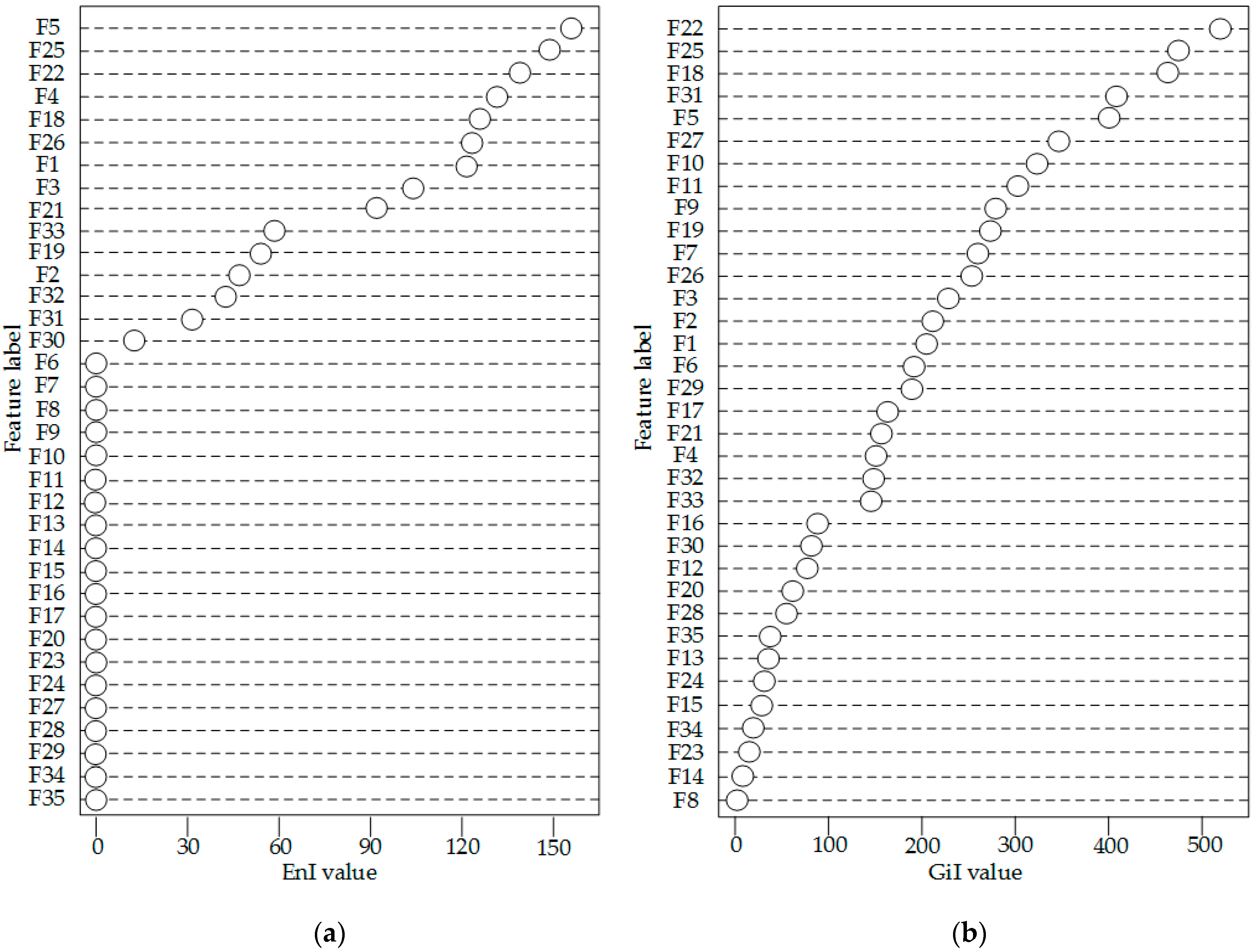
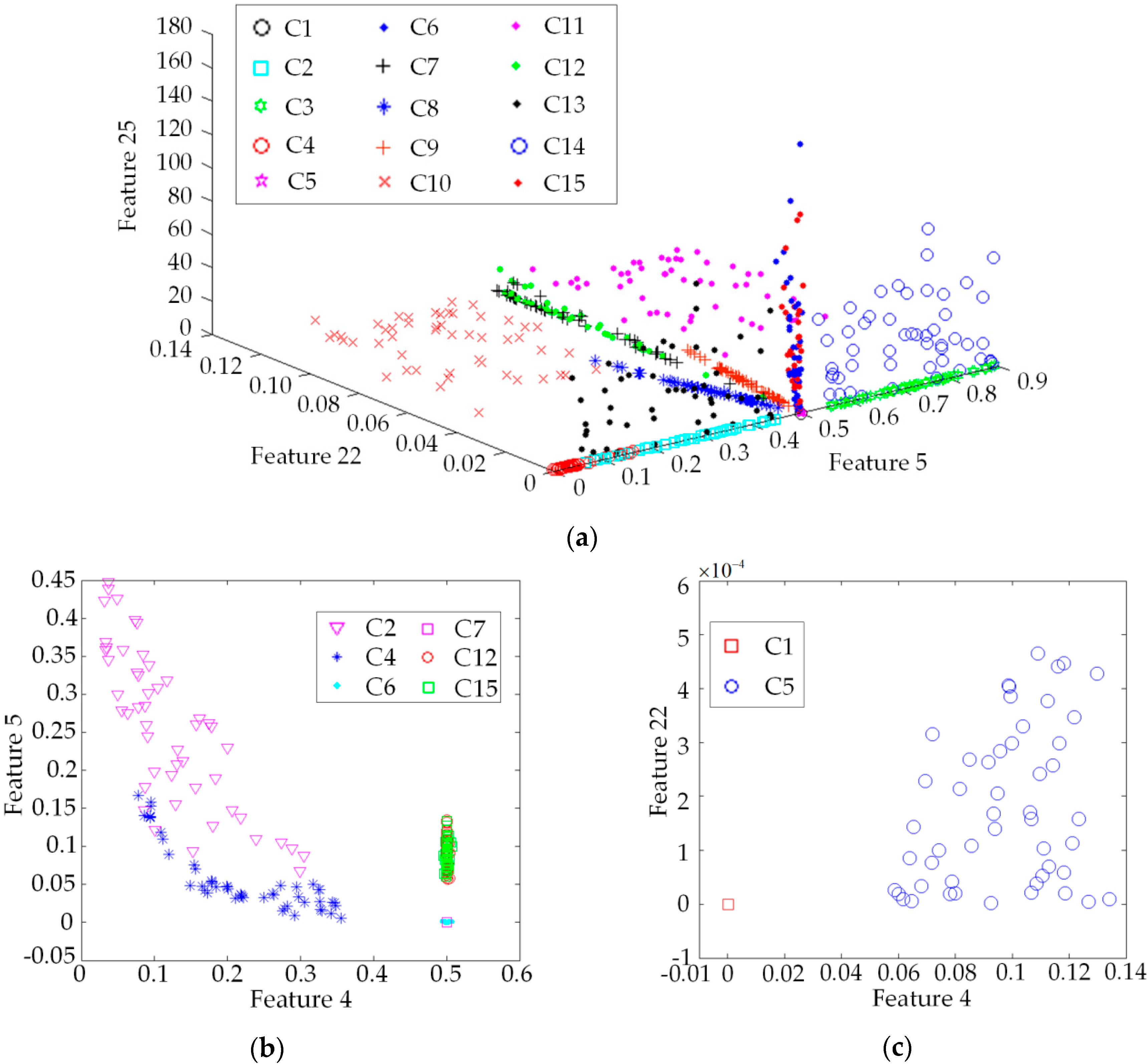
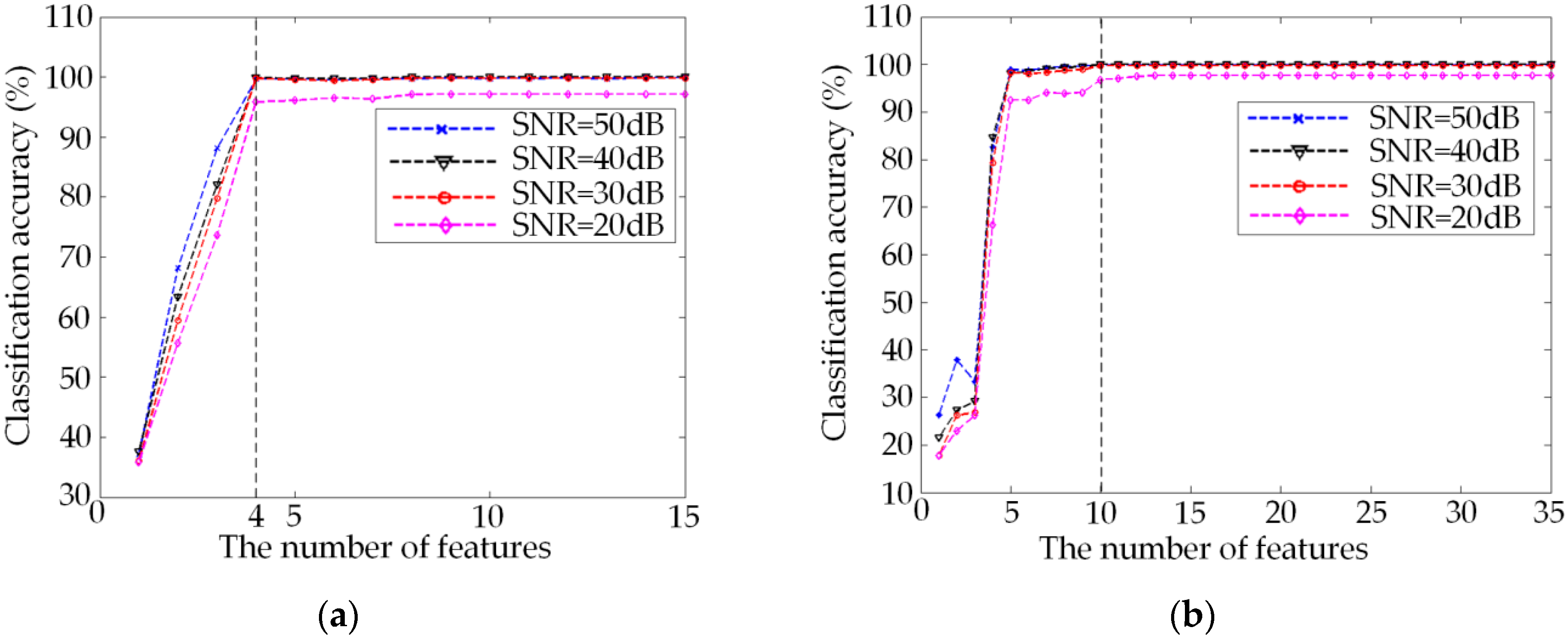
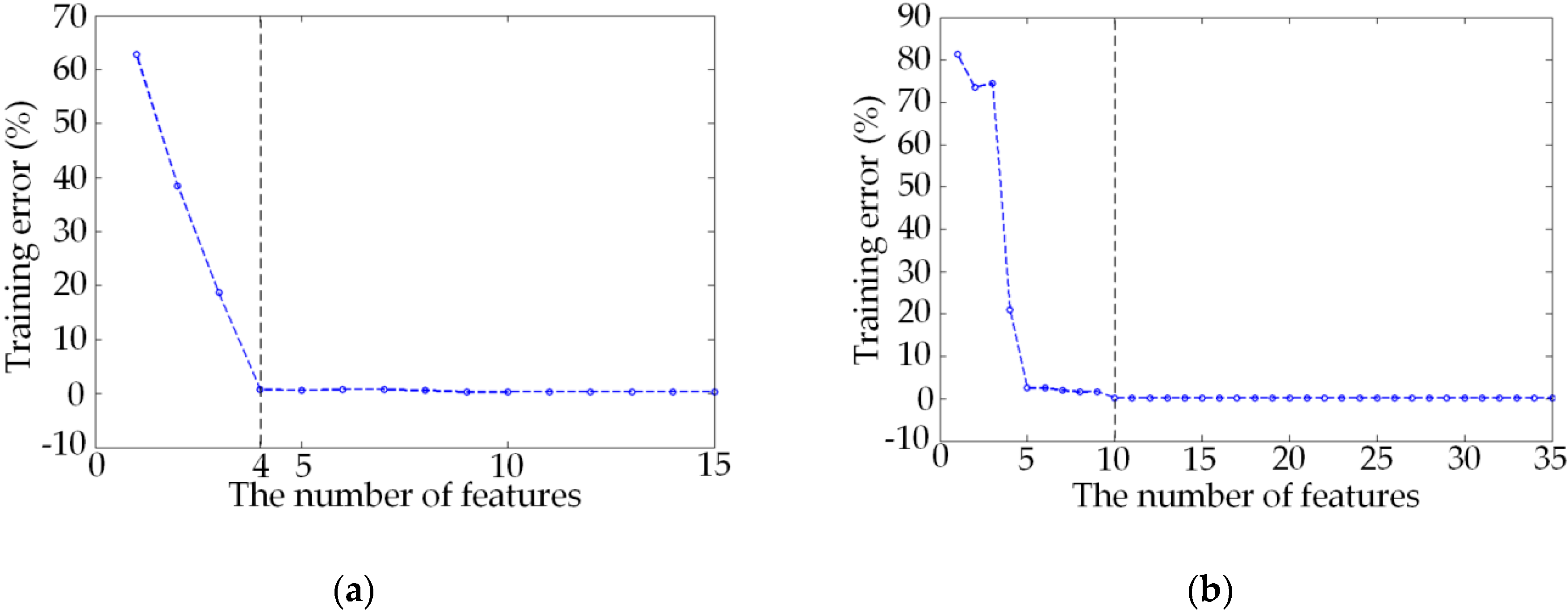
4.2. Feature Selection and Classification Effect Analysis of the New Method

Fifteen types of PQ disturbances with random disturbance parameters and signal-to-noise ratio (SNR) between 50 dB and 20 dB were simulated in Matlab 7.2. Five hundred samples of each type are generated to train the RF classifier for feature selection. Moreover, 100 samples of each type, with random disturbance parameters and the SNR are 50, 40, 30 and 20 dB respectively, are generated to verify the feature selection effect and classification ability of the new method under different noise environments.

According to the new method, features with non-zero EnI value will be added to selected feature subset one after another following the order from big to small of their EnI values. Whenever a feature is added, RF is used to verify the classification effect of this feature subset. Using information gain and Gini index as the basis of the node partition respectively, the two different importances of features are shown in Figure 3a,b. It can be known from Figure 3a that there are 20 features with their EnI value is 0. This means these features have no or very little effect on the node segmentation. Therefore, when searching the feature space, the new method needs only to iterate 15 times while GiI method needs to iterate 35 times. The efficiency of the new method in feature selection is better than GiI based method.

Figure 3. (a) EnI value of features; (b) GiI value of features.

Figure 3. (a) EnI value of features; (b) GiI value of features.

According to Figure 3a, F4, F5, F22 and F25 have the highest EnI value. As explained in Section 4.1, F4 represents the standard deviation of the maximum amplitude of each column in STMM. Then the values of the standard deviation of disturbances such as sag, swell and interruption are large. The values of the STD of steady-state disturbances such as normal voltage, flicker and spike are small respectively, so F4 can divide all kinds of disturbances into two categories. F5 represents the amplitude factor of the maximum amplitude of each column in STMM. Because the values of F5 of swell, sag and other types of disturbances are in different intervals, F5 can distinguish swell and sag with others. F22 represents the maximum value of the intermediate frequency area, and it can distinguish harmonic with other disturbances. F25 represents the energy of local matrix. According to the characteristic that the disturbance frequency of transient is high, F25 can distinguish transient with other disturbances.

Figure 4a–c illustrates the classification performances of combinations of the first four features in Figure 3a in the condition of SNR = $\infty$. Figure 4a shows the scatter plot of combination of F5, F22 and F25. It can be seen that C1 and C5, C2 and C4, C7 and C12 and C6 and C15 exist cross sample. The other types of disturbance are clearly divided. Then F4 and F5 are used for further segmentation as Figure 4b shows. Although C2 and C4 still exists cross in Figure 4b, the cross number is sharply reduced. C7, C12, C6 and C15 are completely separated. As shown in Figure 4c, C1 and C5 can be clearly divided by combination of F4 and F22. Therefore, the four features with the highest EnI value can distinguish 15 types of PQ signal effectively. The validity of the new method is proved.

Figure 4. (a) Scatter plot of F5, F22 and F25; (b) Scatter plot of F4 and F5; (c) Scatter plot of F4 and F22.

Figure 4. (a) Scatter plot of F5, F22 and F25; (b) Scatter plot of F4 and F5; (c) Scatter plot of F4 and F22.

Figure 5 and Figure 6 present the classification effect and training error of different feature subsets with different SNR respectively. With the feature number increased one by one, the classification accuracy is increasing and the training error is decreasing. As shown in Figure 5 and Figure 6, the classification accuracy and the training error tend to be stable when the feature subset dimension of the new method exceeds four, while GiI method needs at least ten features to achieve satisfying classification results.

When the number of selected feature is 4 or 10, respectively, the details of the classification accuracy of EnI method and GiI method are listed in Table 1, Table 2, Table 3 and Table 4. From these four tables, it can be seen that EnI method can achieve higher classification accuracy with the same feature subset under the high noise environment (the SNR of PQ signals is 20 dB).

Figure 5. (a) Classification accuracy of different feature subsets obtained from EnI method; (b) Classification accuracy of different feature subsets obtained from GiI method.

Figure 5. (a) Classification accuracy of different feature subsets obtained from EnI method; (b) Classification accuracy of different feature subsets obtained from GiI method.

Figure 6. (a) Training error of different feature subsets obtained from EnI method; (b) Train error of different feature subsets obtained from GiI method.

Figure 6. (a) Training error of different feature subsets obtained from EnI method; (b) Train error of different feature subsets obtained from GiI method.

Table 1. Classification of new method (the number of feature is 4, SNR is 20 dB).

Class	C0	C1	C2	C3	C4	C5	C6	C7	C8	C9	C10	C11	C12	C13	C14
C0	86	0	0	0	1	9	0	0	4	0	0	0	0	0	0
C1	0	87	0	5	0	0	0	0	0	0	0	0	8	0	0
C2	0	0	94	0	0	0	0	0	0	0	0	0	0	6	0
C3	0	5	0	94	0	0	0	0	0	0	0	0	1	0	0
C4	0	0	0	0	86	0	0	0	0	0	0	0	0	0	14
C5	0	0	0	0	0	99	0	1	0	0	0	0	0	0	0
C6	0	0	0	0	0	0	96	0	3	0	0	1	0	0	0
C7	0	0	0	0	0	0	0	100	0	0	0	0	0	0	0
C8	1	0	0	0	0	0	0	0	96	0	3	0	0	0	0
C9	0	0	0	0	0	0	0	0	0	100	0	0	0	0	0
C10	0	0	0	0	0	0	0	0	0	0	100	0	0	0	0
C11	0	0	0	0	0	0	0	0	0	0	0	100	0	0	0
C12	0	0	0	0	0	0	0	0	0	0	0	0	100	0	0
C13	0	0	0	0	0	0	0	0	0	0	0	0	0	100	0
C14	0	0	0	0	0	0	0	0	0	0	0	0	0	0	100
Comprehensive accuracy: 95.9%

Table 1. Classification of new method (the number of feature is 4, SNR is 20 dB).

Class	C0	C1	C2	C3	C4	C5	C6	C7	C8	C9	C10	C11	C12	C13	C14
C0	86	0	0	0	1	9	0	0	4	0	0	0	0	0	0
C1	0	87	0	5	0	0	0	0	0	0	0	0	8	0	0
C2	0	0	94	0	0	0	0	0	0	0	0	0	0	6	0
C3	0	5	0	94	0	0	0	0	0	0	0	0	1	0	0
C4	0	0	0	0	86	0	0	0	0	0	0	0	0	0	14
C5	0	0	0	0	0	99	0	1	0	0	0	0	0	0	0
C6	0	0	0	0	0	0	96	0	3	0	0	1	0	0	0
C7	0	0	0	0	0	0	0	100	0	0	0	0	0	0	0
C8	1	0	0	0	0	0	0	0	96	0	3	0	0	0	0
C9	0	0	0	0	0	0	0	0	0	100	0	0	0	0	0
C10	0	0	0	0	0	0	0	0	0	0	100	0	0	0	0
C11	0	0	0	0	0	0	0	0	0	0	0	100	0	0	0
C12	0	0	0	0	0	0	0	0	0	0	0	0	100	0	0
C13	0	0	0	0	0	0	0	0	0	0	0	0	0	100	0
C14	0	0	0	0	0	0	0	0	0	0	0	0	0	0	100
Comprehensive accuracy: 95.9%

Table 2. Classification of GiI method (the number of feature is 4, SNR is 20 dB).

Class	C0	C1	C2	C3	C4	C5	C6	C7	C8	C9	C10	C11	C12	C13	C14
C0	37	0	57	0	0	3	0	0	1	0	0	0	0	2	0
C1	0	63	0	22	7	0	0	0	0	0	0	0	8	0	0
C2	10	0	82	0	0	1	0	2	0	0	0	0	0	5	0
C3	0	1	0	98	0	0	0	0	0	0	0	0	1	0	0
C4	0	1	0	0	84	0	0	0	0	0	0	0	0	0	15
C5	0	0	0	0	0	51	0	0	0	0	0	0	0	49	0
C6	0	0	0	0	0	0	33	3	0	0	32	32	0	0	0
C7	0	0	0	0	0	0	0	80	0	2	0	17	0	1	0
C8	1	0	1	0	0	0	4	64	28	0	0	2	0	0	0
C9	0	0	0	0	0	0	0	0	0	86	0	14	0	0	0
C10	0	0	0	0	0	0	30	6	0	0	29	35	0	0	0
C11	0	0	0	0	0	0	3	1	0	16	6	74	0	0	0
C12	0	0	0	0	0	0	0	0	0	0	0	0	85	0	15
C13	0	0	0	0	0	33	0	0	0	0	0	0	0	67	0
C14	0	0	0	0	0	0	0	0	0	0	0	0	2	0	98
Comprehensive accuracy: 66.3%

Table 2. Classification of GiI method (the number of feature is 4, SNR is 20 dB).

Class	C0	C1	C2	C3	C4	C5	C6	C7	C8	C9	C10	C11	C12	C13	C14
C0	37	0	57	0	0	3	0	0	1	0	0	0	0	2	0
C1	0	63	0	22	7	0	0	0	0	0	0	0	8	0	0
C2	10	0	82	0	0	1	0	2	0	0	0	0	0	5	0
C3	0	1	0	98	0	0	0	0	0	0	0	0	1	0	0
C4	0	1	0	0	84	0	0	0	0	0	0	0	0	0	15
C5	0	0	0	0	0	51	0	0	0	0	0	0	0	49	0
C6	0	0	0	0	0	0	33	3	0	0	32	32	0	0	0
C7	0	0	0	0	0	0	0	80	0	2	0	17	0	1	0
C8	1	0	1	0	0	0	4	64	28	0	0	2	0	0	0
C9	0	0	0	0	0	0	0	0	0	86	0	14	0	0	0
C10	0	0	0	0	0	0	30	6	0	0	29	35	0	0	0
C11	0	0	0	0	0	0	3	1	0	16	6	74	0	0	0
C12	0	0	0	0	0	0	0	0	0	0	0	0	85	0	15
C13	0	0	0	0	0	33	0	0	0	0	0	0	0	67	0
C14	0	0	0	0	0	0	0	0	0	0	0	0	2	0	98
Comprehensive accuracy: 66.3%

Table 3. Classification of new method (the number of feature is 10, SNR is 20 dB).

Class	C0	C1	C2	C3	C4	C5	C6	C7	C8	C9	C10	C11	C12	C13	C14
C0	91	0	0	0	0	9	0	0	0	0	0	0	0	0	0
C1	0	87	0	5	0	0	0	0	0	0	0	0	8	0	0
C2	0	0	94	0	0	0	0	0	0	0	0	0	0	6	0
C3	0	1	0	98	0	0	0	0	0	0	0	0	1	0	0
C4	0	0	0	0	86	0	0	0	0	0	0	0	0	0	14
C5	0	0	0	0	0	100	0	0	0	0	0	0	0	0	0
C6	0	0	0	0	0	0	100	0	0	0	0	0	0	0	0
C7	0	0	0	0	0	0	0	100	0	0	0	0	0	0	0
C8	0	0	0	0	0	0	0	0	100	0	0	0	0	0	0
C9	0	0	0	0	0	0	0	0	0	100	0	0	0	0	0
C10	0	0	0	0	0	0	0	0	0	0	100	0	0	0	0
C11	0	0	0	0	0	0	0	0	0	0	0	100	0	0	0
C12	0	0	0	0	0	0	0	0	0	0	0	0	100	0	0
C13	0	0	0	0	0	0	0	0	0	0	0	0	0	100	0
C14	0	0	0	0	0	0	0	0	0	0	0	0	0	0	100
Comprehensive accuracy: 97.1%

Table 3. Classification of new method (the number of feature is 10, SNR is 20 dB).

Class	C0	C1	C2	C3	C4	C5	C6	C7	C8	C9	C10	C11	C12	C13	C14
C0	91	0	0	0	0	9	0	0	0	0	0	0	0	0	0
C1	0	87	0	5	0	0	0	0	0	0	0	0	8	0	0
C2	0	0	94	0	0	0	0	0	0	0	0	0	0	6	0
C3	0	1	0	98	0	0	0	0	0	0	0	0	1	0	0
C4	0	0	0	0	86	0	0	0	0	0	0	0	0	0	14
C5	0	0	0	0	0	100	0	0	0	0	0	0	0	0	0
C6	0	0	0	0	0	0	100	0	0	0	0	0	0	0	0
C7	0	0	0	0	0	0	0	100	0	0	0	0	0	0	0
C8	0	0	0	0	0	0	0	0	100	0	0	0	0	0	0
C9	0	0	0	0	0	0	0	0	0	100	0	0	0	0	0
C10	0	0	0	0	0	0	0	0	0	0	100	0	0	0	0
C11	0	0	0	0	0	0	0	0	0	0	0	100	0	0	0
C12	0	0	0	0	0	0	0	0	0	0	0	0	100	0	0
C13	0	0	0	0	0	0	0	0	0	0	0	0	0	100	0
C14	0	0	0	0	0	0	0	0	0	0	0	0	0	0	100
Comprehensive accuracy: 97.1%

Table 4. Classification of GiI method (the number of feature is 10, SNR is 20 dB).

Class	C0	C1	C2	C3	C4	C5	C6	C7	C8	C9	C10	C11	C12	C13	C14
C0	90	0	0	0	0	7	0	0	3	0	0	0	0	0	0
C1	0	90	0	4	0	0	0	0	0	0	0	0	6	0	0
C2	0	0	94	0	0	0	0	0	0	0	0	0	0	6	0
C3	0	3	0	97	0	0	0	0	0	0	0	0	0	0	0
C4	0	0	0	0	91	0	0	0	0	0	0	0	0	0	9
C5	0	0	0	0	0	100	0	0	0	0	0	0	0	0	0
C6	0	0	0	0	0	0	94	0	1	0	0	5	0	0	0
C7	0	0	0	0	0	0	0	100	0	0	0	0	0	0	0
C8	1	0	0	0	0	0	0	0	99	0	0	0	0	0	0
C9	0	0	0	0	0	0	0	1	0	99	0	0	0	0	0
C10	0	0	0	0	0	0	0	0	0	0	100	0	0	0	0
C11	0	0	0	0	0	0	0	0	0	2	0	98	0	0	0
C12	0	0	0	0	0	0	0	0	0	0	0	0	100	0	0
C13	0	0	0	0	0	0	0	0	0	0	0	0	0	100	0
C14	0	0	0	0	0	0	0	0	0	0	0	0	0	0	100
Comprehensive accuracy: 96.8%

Table 4. Classification of GiI method (the number of feature is 10, SNR is 20 dB).

Class	C0	C1	C2	C3	C4	C5	C6	C7	C8	C9	C10	C11	C12	C13	C14
C0	90	0	0	0	0	7	0	0	3	0	0	0	0	0	0
C1	0	90	0	4	0	0	0	0	0	0	0	0	6	0	0
C2	0	0	94	0	0	0	0	0	0	0	0	0	0	6	0
C3	0	3	0	97	0	0	0	0	0	0	0	0	0	0	0
C4	0	0	0	0	91	0	0	0	0	0	0	0	0	0	9
C5	0	0	0	0	0	100	0	0	0	0	0	0	0	0	0
C6	0	0	0	0	0	0	94	0	1	0	0	5	0	0	0
C7	0	0	0	0	0	0	0	100	0	0	0	0	0	0	0
C8	1	0	0	0	0	0	0	0	99	0	0	0	0	0	0
C9	0	0	0	0	0	0	0	1	0	99	0	0	0	0	0
C10	0	0	0	0	0	0	0	0	0	0	100	0	0	0	0
C11	0	0	0	0	0	0	0	0	0	2	0	98	0	0	0
C12	0	0	0	0	0	0	0	0	0	0	0	0	100	0	0
C13	0	0	0	0	0	0	0	0	0	0	0	0	0	100	0
C14	0	0	0	0	0	0	0	0	0	0	0	0	0	0	100
Comprehensive accuracy: 96.8%

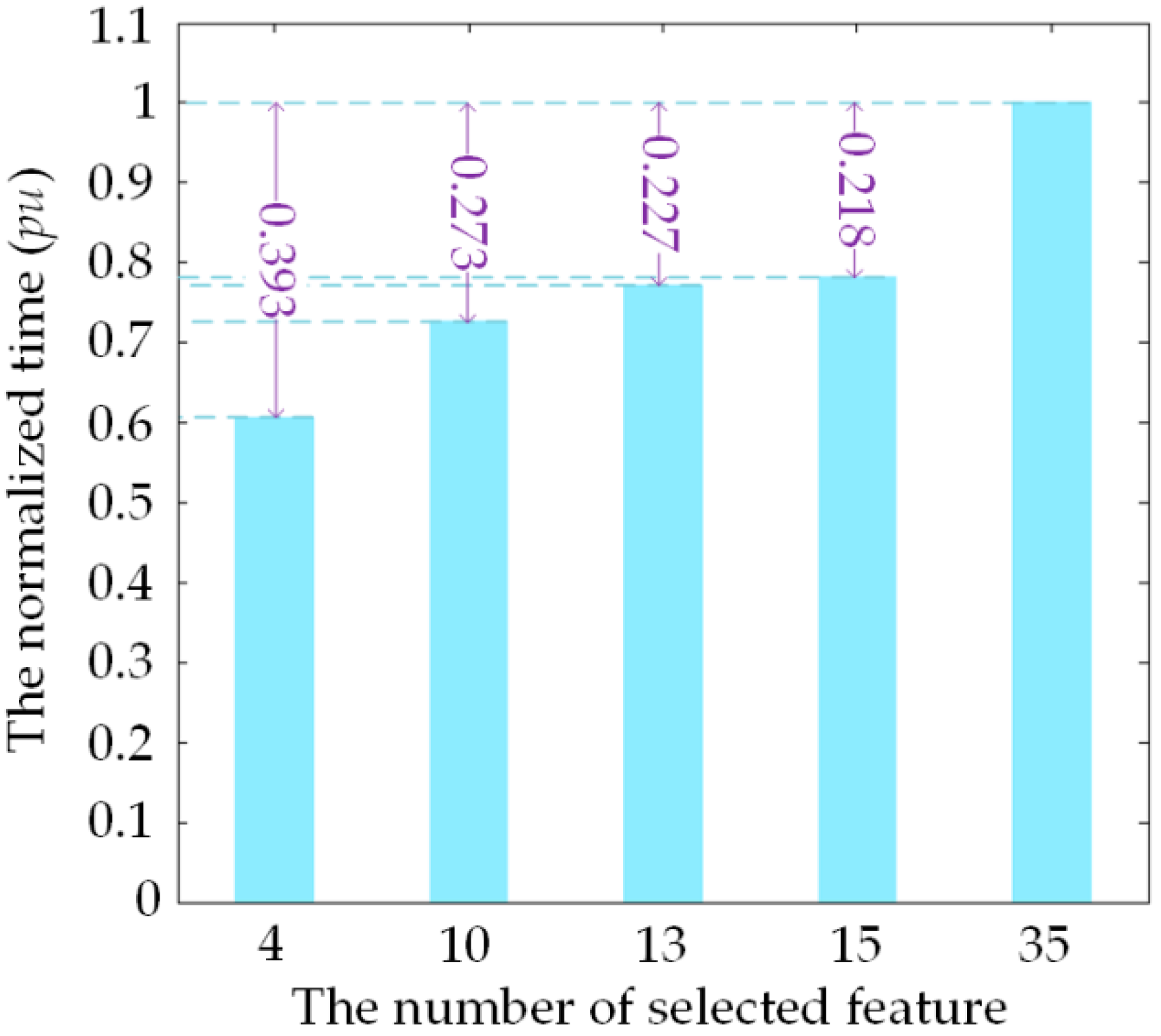
4.3. Comparison Experiment and Analysis

The feature selection result of the new method is compared with GiI method, SFS algorithm [35] and sequential backward search (SBS) [36] to testify the validity of the new approach. The number of selected feature based on GiI method, SFS method and SBS method are 10, 13 and 15 respectively. The new method considers two cases, including the dimension of the feature subset are 4 and 10 respectively. Moreover, the original feature set is used as a contrast as well.

The selected features after feature selection segment by the new method are {F4,F5,F22,F25} and {F1,F3,F4,F5,F18,F21,F22,F25,F26, F33}, respectively.

The selected features after feature selection segment by the GiI method are {F5,F9,F10,F11,F18,F19,F22,F25,F27,F31}.

The selected features after feature selection segment by the SFS method are {F2,F4,F5,F7,F10,F16,F18,F19,F22,F26,F27,F29,F31}.

The selected features after feature selection segment by the SBS method is {F1,F3,F4,F6,F11,F13,F18,F22,F23,F25,F27,F28,F29,F31,F33}.

For the sake of verifying the validity of the feature selection results of the new method, four kinds of classifier, including RF, SVM [14], PNN [13] and DT, are used to classify 15 kinds of PQ signals under the condition of different noise environments and different feature subsets. The DT classifier is constructed by rpart software package in R project. The classification results are shown in Table 5.

Table 5. Comparison of feature selection method.

SNR	Feature Selection Method	The Number of Features	Classification Accuracy(%)
			RF	SVM	NN	DT
50 dB	EnI + SFS	4	99.7	95.5	98.9	98.1
	GiI + SFS	4	82.6	74.6	76.1	75.3
	EnI + SFS	10	99.9	98.6	99.6	99.0
	GiI + SFS	10	99.9	98.5	99.7	98.9
	SFS	13	99.4	98.3	99.5	98.3
	SBS	15	99.8	98.7	99.5	99.2
	ALL	35	99.9	98.9	97.6	99.5
40 dB	EnI + SFS	4	99.9	96.1	99.2	99.4
	GiI + SFS	4	84.7	72.1	77.2	76.7
	EnI + SFS	10	100	96.8	99.8	99.7
	GiI + SFS	10	100	98.4	99.8	99.4
	SFS	13	99.6	98.4	99.6	98.7
	SBS	15	99.9	98.5	99.7	99.6
	ALL	35	100	99.3	98.2	99.9
30 dB	EnI + SFS	4	99.7	95.8	99.1	98.5
	GiI + SFS	4	79.3	70.1	71.9	72.1
	EnI + SFS	10	99.7	96.2	99.6	99.0
	GiI + SFS	10	99.7	97.9	99.5	99.0
	SFS	13	98.8	97.7	99.1	98.0
	SBS	15	99.7	97.9	99.5	99.1
	ALL	35	99.7	98.2	97.6	99.6
20 dB	EnI + SFS	4	95.9	94.8	94.2	92.5
	GiI + SFS	4	66.3	59.5	63.5	60.9
	EnI + SFS	10	97.1	95.9	95.2	93.9
	GiI + SFS	10	96.8	90.3	95.0	85.5
	SFS	13	90.3	90.7	88.7	80.5
	SBS	15	98.5	88.6	94.8	94.2
	ALL	35	97.6	90.9	94.5	95.0

Table 5. Comparison of feature selection method.

SNR	Feature Selection Method	The Number of Features	Classification Accuracy(%)
			RF	SVM	NN	DT
50 dB	EnI + SFS	4	99.7	95.5	98.9	98.1
	GiI + SFS	4	82.6	74.6	76.1	75.3
	EnI + SFS	10	99.9	98.6	99.6	99.0
	GiI + SFS	10	99.9	98.5	99.7	98.9
	SFS	13	99.4	98.3	99.5	98.3
	SBS	15	99.8	98.7	99.5	99.2
	ALL	35	99.9	98.9	97.6	99.5
40 dB	EnI + SFS	4	99.9	96.1	99.2	99.4
	GiI + SFS	4	84.7	72.1	77.2	76.7
	EnI + SFS	10	100	96.8	99.8	99.7
	GiI + SFS	10	100	98.4	99.8	99.4
	SFS	13	99.6	98.4	99.6	98.7
	SBS	15	99.9	98.5	99.7	99.6
	ALL	35	100	99.3	98.2	99.9
30 dB	EnI + SFS	4	99.7	95.8	99.1	98.5
	GiI + SFS	4	79.3	70.1	71.9	72.1
	EnI + SFS	10	99.7	96.2	99.6	99.0
	GiI + SFS	10	99.7	97.9	99.5	99.0
	SFS	13	98.8	97.7	99.1	98.0
	SBS	15	99.7	97.9	99.5	99.1
	ALL	35	99.7	98.2	97.6	99.6
20 dB	EnI + SFS	4	95.9	94.8	94.2	92.5
	GiI + SFS	4	66.3	59.5	63.5	60.9
	EnI + SFS	10	97.1	95.9	95.2	93.9
	GiI + SFS	10	96.8	90.3	95.0	85.5
	SFS	13	90.3	90.7	88.7	80.5
	SBS	15	98.5	88.6	94.8	94.2
	ALL	35	97.6	90.9	94.5	95.0

The feature selection methods based on EnI and GiI are compared according to Table 5. When RF is used as the classifier, and the selected feature number of EnI method is 4, the classification accuracy is almost close to GiI method with 10 features. When the selected feature number of EnI method is equal to GiI method, the accuracy of these two methods under the condition that the SNR is higher than 30 dB are the same, but the accuracy of EnI method under the condition that the SNR is 20 dB exceeds 0.3% compared to GiI method. It is proved that the new method based on EnI has better effect than GiI based method with RF based classifier. Meanwhile, when SNR is 20 dB, the SBS method can achieve the classification accuracy of 98.5%. However, when taking classification accuracy under all conditions and the efficiency of feature selection and extraction into consideration, EnI method is still thought to be better than SBS method. It can also be seen that the new method can use the same feature subset to achieve satisfying classification accuracy under different noise environments. This overcomes the disadvantage that existing research [15] needs to select different feature subsets under different noise environments. Meanwhile, when RF is used as classifier and the dimension of the selected feature subset increases from 4 to 10, the classification accuracy of high SNR environment has not improved, but the classification accuracy of SNR is 20 dB has improved 1.2%. Therefore, different feature subsets can be selected according to the demand of classification accuracy and efficiency in practical work.

The classification ability of different classifiers can also be analyzed using Table 5. As shown in Table 5, when compared to the other three classifiers, RF performs better on the new test sets. The best classification accuracy can only be achieved by using RF as the classifier no matter what level of the noise environment is. When the SNR is 50 dB, and the feature selection methods are EnI + SFS (the number of selected feature is 10), GiI + SFS (the number of selected feature is 10) and ALL, RF can achieve the classification accuracy of 99.9%. When the SNR is 40 dB, and the feature selection methods are EnI + SFS (the number of selected feature is 10) and GiI + SFS (the number of selected feature is 10), RF can achieve the classification accuracy of 100%. When the SNR is 30 dB, and the feature selection methods are EnI + SFS (the number of selected feature is 4), EnI + SFS (the number of selected feature is 10), GiI + SFS (the number of selected feature is 10) and ALL, RF can achieve the classification accuracy of 99.7%. When the noise environment is high (SNR is 20 dB), and the feature selection method is SBS, the RF classification accuracy is higher than the SVM of 9.9%, and is higher than the other two classifiers of 3.7% and 4.3% respectively. All these prove that RF has higher anti-noise ability, and is more suitable for the application under high noise environment. Moreover, the RF classification accuracy is higher than the DT under any condition, which proves that RF has better generalization ability than DT.

Besides classification accuracy, the impact on classification efficiency by feature selection is also analyzed. In practical application, the original PQ signals have the need for ST process after they are collected. Then the corresponding features are extracted according to the ST results. Finally, the extracted features are used as the input of the well trained classifier to output the disturbance type. Therefore, feature selection can effectively reduce the computing time of features and complexity of classifier. When the number of selected feature are 4, 10, 13, 15 and 35 respectively, the normalized time that 50 new test sets of original disturbance signals consumed from ST process to disturbance type output is shown in Figure 7. The whole time of signals recognized by 35 features were treated as the standard time (1 pu).

From Figure 7, it can be seen that, the total classificaiton time reduces significantly with the decrease of feature number. When the number of selected feature decreased from 35 to 4, the total classificaiton time can reduce by 39.3%. When the number of selected feature decreased from 35 to 10, the total classification time can reduce by 27.3%. It proves that feature selection improves the classification efficiency of the classifier effectively.

Figure 7. The normalized time of different selected feature number.

Figure 7. The normalized time of different selected feature number.

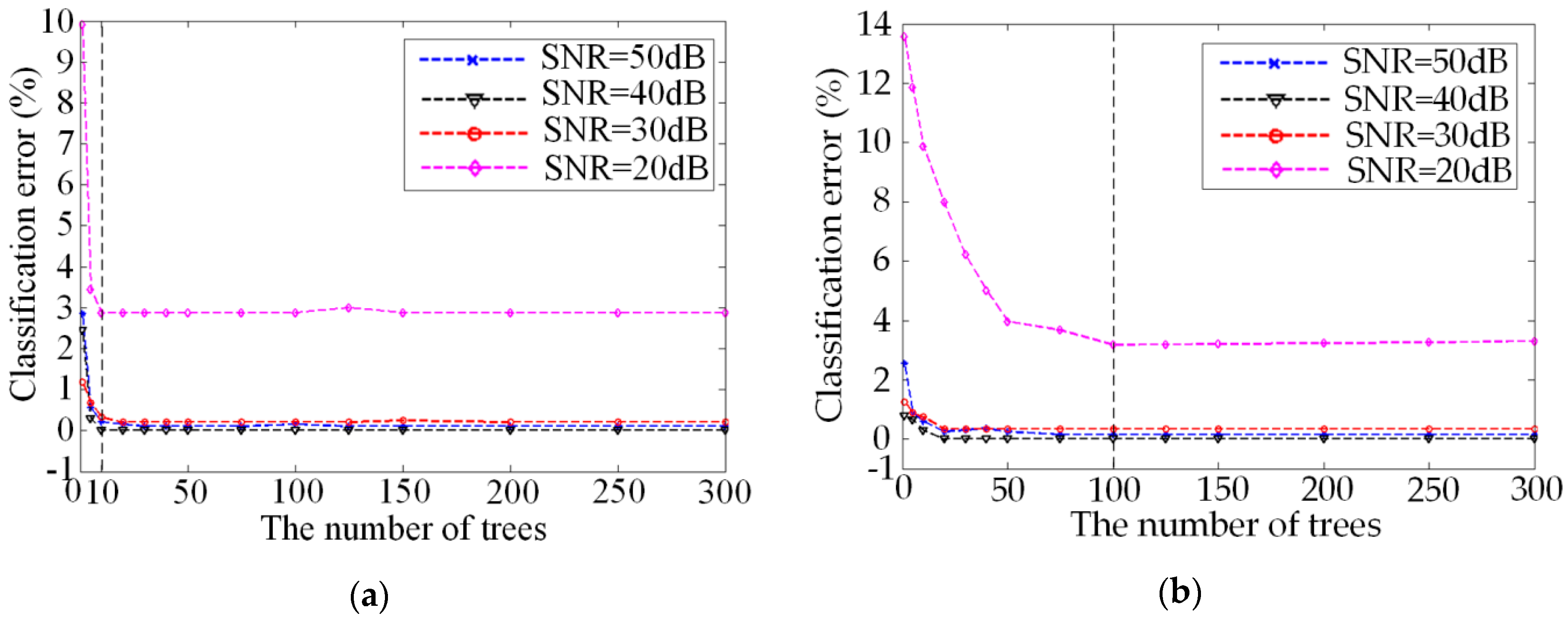
4.4. The Determination of Tree Number of RF Classifier

The number of the tree determines the scale of RF. With the increasing of tree number, the generalization error becomes smaller and EnI analysis of features becomes more accurate. Therefore, the classification performance will be better. The number of trees in RF is set to 300 during the feature selection process. However, too many trees will affect the efficiency of classification. Then it is necessary to analyze the influence of the number of the trees on the classification error in order to determine the optimal RF scale based on the optimized feature subset. Figure 8a,b show the relationship between the number of trees and classification error by different feature selection method.

Figure 8. (a) Classification error of different scale of RF of EnI method; (b) Classification error of different scale of RF of GiI method.

Figure 8. (a) Classification error of different scale of RF of EnI method; (b) Classification error of different scale of RF of GiI method.

In Figure 8a, when the tree number is over 10, the classification error is tending to be stable, while GiI method needs at least 100 trees in Figure 8b. The new method has simpler structure than GiI based RF with same classification accuracy. Meanwhile, with the increase of the tree number, the time spent on RF classification will be improved. Finally, the number of trees in RF is determined to be 10 during classification process.

4.5. Affection of Signal Processing Method on Classification Accuracy

The influence of the signal processing method for PQ signals will also be considered. Different signal processing methods will affect the classification accuracy of PQ disturbance signals. Therefore, after the new feature selection method and RF classifier are proved to be effective, the classification accuracy of discrete wavelet transform (DWT) [37] and wavelet package transform (WPT) [38] are compared to ST. The new method is chosen as the feature selection and classification method.

In the contrast experiment, the features of DWT based method are extracted refers to literature [37]. The fourth-order Daubechies wavelet (db-4) was chosen as the mother wavelet function. Then a 9-level multiresolution decomposition process is performed to the original signals. According to the detail coefficients at each level and the approximate coefficient at the last level, 90 features are extracted. The feature extraction methods of DWT are shown in Table 6.

Table 6. Feature extraction methods based on DWT [37].

Feature Extraction Methods Based on DWT
Mean	${\mu }_i=\frac{1}{N}{\displaystyle {\sum }_{j=1}^N{C}_{ij}}$	Energy	$E_i={{\displaystyle {\sum }_{j=1}^N\left|C_{ij}\right|}}^2$
Standard deviation	${\sigma }_i={\left(\frac{1}{N}{\displaystyle {\sum }_{j=1}^N{(C_{ij}-{\mu }_i)}^2}\right)}^{\frac{1}{2}}$	Shannon entropy	$S{E}_i=-{\displaystyle {\sum }_{j=1}^N{C}_{ij}^2\log (C_{ij}^2)}$
Skewness	$S{K}_i=\sqrt{\frac{1}{6N}}{{\displaystyle {\sum }_{j=1}^N\left(\frac{C_{ij}-{\mu }_i}{{\sigma }_i}\right)}}^3$	Log energy entropy	$LO{E}_i={\displaystyle {\sum }_{j=1}^N\log (C_{ij}^2)}$
Kurtosis	$KR{T}_i=\sqrt{\frac{N}{24}}\left(\frac{1}{N}{{\displaystyle {\sum }_{j=1}^N\left(\frac{C_{ij}-{\mu }_i}{{\sigma }_i}\right)}}^4-3\right)$	Norm entropy	$N{E}_i={{\displaystyle {\sum }_{j=1}^N(C_{ij})}}^{P}1\le P$
RMS	$rm{s}_i=\sqrt{\frac{1}{N}{\displaystyle {\sum }_{j=1}^N{C}_{ij}^2}}$

Table 6. Feature extraction methods based on DWT [37].

Feature Extraction Methods Based on DWT
Mean	${\mu }_i=\frac{1}{N}{\displaystyle {\sum }_{j=1}^N{C}_{ij}}$	Energy	$E_i={{\displaystyle {\sum }_{j=1}^N\left|C_{ij}\right|}}^2$
Standard deviation	${\sigma }_i={\left(\frac{1}{N}{\displaystyle {\sum }_{j=1}^N{(C_{ij}-{\mu }_i)}^2}\right)}^{\frac{1}{2}}$	Shannon entropy	$S{E}_i=-{\displaystyle {\sum }_{j=1}^N{C}_{ij}^2\log (C_{ij}^2)}$
Skewness	$S{K}_i=\sqrt{\frac{1}{6N}}{{\displaystyle {\sum }_{j=1}^N\left(\frac{C_{ij}-{\mu }_i}{{\sigma }_i}\right)}}^3$	Log energy entropy	$LO{E}_i={\displaystyle {\sum }_{j=1}^N\log (C_{ij}^2)}$
Kurtosis	$KR{T}_i=\sqrt{\frac{N}{24}}\left(\frac{1}{N}{{\displaystyle {\sum }_{j=1}^N\left(\frac{C_{ij}-{\mu }_i}{{\sigma }_i}\right)}}^4-3\right)$	Norm entropy	$N{E}_i={{\displaystyle {\sum }_{j=1}^N(C_{ij})}}^{P}1\le P$
RMS	$rm{s}_i=\sqrt{\frac{1}{N}{\displaystyle {\sum }_{j=1}^N{C}_{ij}^2}}$

In Table 6, i = 1,2,L,…,l represents multi resolution level, and N stands for the number of details or approximate coefficients at each multi resolution level.

The features extracted from WPT refer to literature [38]. The fourth-order Daubechies wavelet (db-4) was also chosen as the mother wavelet function. Then 16 wavelet coefficients can be obtained by performing a 4-level decomposition process, and 96 features can be extracted according to these coefficients. The feature extraction methods of WPT are shown in Table 7.

Table 7. Feature extraction methods based on WPT [38].

Feature Extraction Methods Based on WPT
Mean	${\mu }_j=\frac{1}{M}{\displaystyle {\sum }_{l=1}^M{C}_{jl}}$	Kurtosis	$KR{T}_j=\frac{E{(C_{jl}-{\mu }_j)}^4}{{\sigma }_j^4}$
Standard deviation	${\sigma }_j={\left(\frac{1}{M-1}{\displaystyle {\sum }_{l=1}^M{(C_{jl}-{\mu }_j)}^2}\right)}^{\frac{1}{2}}$	Energy	$E{D}_j={{\displaystyle {\sum }_{l=1}^M\left|C_{jl}\right|}}^2$
Skewness	$S{K}_j=\frac{E{(C_{jl}-{\mu }_j)}^3}{{\sigma }_j^3}$	Entropy	$EN{T}_j=-{\displaystyle {\sum }_{l=1}^M{C}_{jl}^2\log (C_{jl}^2)}$

Table 7. Feature extraction methods based on WPT [38].

Feature Extraction Methods Based on WPT
Mean	${\mu }_j=\frac{1}{M}{\displaystyle {\sum }_{l=1}^M{C}_{jl}}$	Kurtosis	$KR{T}_j=\frac{E{(C_{jl}-{\mu }_j)}^4}{{\sigma }_j^4}$
Standard deviation	${\sigma }_j={\left(\frac{1}{M-1}{\displaystyle {\sum }_{l=1}^M{(C_{jl}-{\mu }_j)}^2}\right)}^{\frac{1}{2}}$	Energy	$E{D}_j={{\displaystyle {\sum }_{l=1}^M\left|C_{jl}\right|}}^2$
Skewness	$S{K}_j=\frac{E{(C_{jl}-{\mu }_j)}^3}{{\sigma }_j^3}$	Entropy	$EN{T}_j=-{\displaystyle {\sum }_{l=1}^M{C}_{jl}^2\log (C_{jl}^2)}$

In Table 7, j = 1,2,L,…,k represents the number of nodes at the fourth decomposition level, and $M$ is the number of coefficients in each decomposed data.

After the original feature subsets are obtained, the new feature selection stategy put forward in this paper is adopted to select useful features as well. The number of features selected from the original feature subsets of DWT and WPT are 23 and 27, respectively, and the descriptions of these two optimal feature subsets are shown in Table 8 and Table 9, respectively. Finally, the two optimal feature subsets are used as the input of the RF to train the classifier. The classification accuracy of the classifier is shown in Table 10.

Table 8. The selected features extracted from DWT method.

The Numbers and Names of the Selected Features Extracted from DWT Method
7	7th level of mean	37	7th level of kurtosis	65	5th level of Shannon entropy
9	9th level of mean	44	4th level of RMS	67	7th level of Shannon entropy
14	4th level of Std. Deviation	45	5th level of RMS	84	4th level of norm entropy
15	5th level of Std. Deviation	48	8th level of RMS	85	5th level of norm entropy
20	App. level of Std. deviation	54	4th level of energy	86	6th level of norm entropy
27	7th level of Skewness	55	5th level of energy	87	7th level of norm entropy
32	2th level of kurtosis	58	8th level of energy	90	App. level of norm entropy
35	5th level of kurtosis	64	4th level of Shannon entropy

Table 8. The selected features extracted from DWT method.

The Numbers and Names of the Selected Features Extracted from DWT Method
7	7th level of mean	37	7th level of kurtosis	65	5th level of Shannon entropy
9	9th level of mean	44	4th level of RMS	67	7th level of Shannon entropy
14	4th level of Std. Deviation	45	5th level of RMS	84	4th level of norm entropy
15	5th level of Std. Deviation	48	8th level of RMS	85	5th level of norm entropy
20	App. level of Std. deviation	54	4th level of energy	86	6th level of norm entropy
27	7th level of Skewness	55	5th level of energy	87	7th level of norm entropy
32	2th level of kurtosis	58	8th level of energy	90	App. level of norm entropy
35	5th level of kurtosis	64	4th level of Shannon entropy

Table 9. The selected features extracted from WPT method.

The Numbers and Names of the Selected Features Extracted from WPT Method
1	Mean of 1st node	49	kurtosis of 1st node	61	kurtosis of 13th node
2	Mean of 2nd node	50	kurtosis of 2nd node	62	kurtosis of 14th node
4	Mean of 4th node	51	kurtosis of 3rd node	64	kurtosis of 16th node
7	Mean of 7th node	52	kurtosis of 4th node	65	energy of 1st node
17	Std. deviation of 1st node	53	kurtosis of 5th node	66	energy of 2ndnode
18	Std. deviation of 2nd node	54	kurtosis of 6th node	68	energy of 4th node
20	Std. deviation of 4th node	55	kurtosis of 7th node	81	entropy of 1st node
33	skewness of 1st node	56	kurtosis of 8th node	82	entropy of 2nd node
34	skewness of 2nd node	58	kurtosis of 10th node	84	entropy of 4th node

Table 9. The selected features extracted from WPT method.

The Numbers and Names of the Selected Features Extracted from WPT Method
1	Mean of 1st node	49	kurtosis of 1st node	61	kurtosis of 13th node
2	Mean of 2nd node	50	kurtosis of 2nd node	62	kurtosis of 14th node
4	Mean of 4th node	51	kurtosis of 3rd node	64	kurtosis of 16th node
7	Mean of 7th node	52	kurtosis of 4th node	65	energy of 1st node
17	Std. deviation of 1st node	53	kurtosis of 5th node	66	energy of 2ndnode
18	Std. deviation of 2nd node	54	kurtosis of 6th node	68	energy of 4th node
20	Std. deviation of 4th node	55	kurtosis of 7th node	81	entropy of 1st node
33	skewness of 1st node	56	kurtosis of 8th node	82	entropy of 2nd node
34	skewness of 2nd node	58	kurtosis of 10th node	84	entropy of 4th node

Table 10. Effect of different signal processing methods for PQ classification.

SNR	Feature Selection	Classification Accuracy with Different Signal Processing Method(%)
		ST	DWT	WPT
50 dB	No	99.7	98.4	95.5
	Yes	99.9	97.5	94.2
40 dB	No	100	98.8	96.4
	Yes	100	98.9	94.8
30 dB	No	99.7	97.1	94.0
	Yes	99.7	96.7	91.5
20 dB	No	97.6	83.5	82.9
	Yes	97.1	85.8	82.6

Table 10. Effect of different signal processing methods for PQ classification.

SNR	Feature Selection	Classification Accuracy with Different Signal Processing Method(%)
		ST	DWT	WPT
50 dB	No	99.7	98.4	95.5
	Yes	99.9	97.5	94.2
40 dB	No	100	98.8	96.4
	Yes	100	98.9	94.8
30 dB	No	99.7	97.1	94.0
	Yes	99.7	96.7	91.5
20 dB	No	97.6	83.5	82.9
	Yes	97.1	85.8	82.6

From Table 10, it can be clearly seen that the method with ST can achieve higher classification accuracy than the other signal processing methods under any conditions. When SNR is 20 dB and there is no feature selection process, the classification accuracy of ST based method is higher than DWT and WPT of 14.1% and 14.7%, respectively. If the feature selection process is performed, the classification accuracy of ST based method is higher than DWT and WPT of 11.3% and 14.5%, respectively. These prove that ST has good anti-noise ability. It is reasonable to use ST as the signal processing method in the new approach.

5. Conclusions

This paper proposes a PQ signal feature selection and classification approach based on an EnI based RF. The innovations in this article are listed as follows:

(1)

The EnI based feature selection method used in the new approach calculated the EnI value during the training process of RF. These values provide the theoretical basis for SFS search strategy and improve the efficiency of feature search strategy than GiI based method.

(2)

RF is used for disturbance identification. While remains the classification accuracy and efficiency as DT method, RF also increases the generalization ability of the PQ classifier.

(3)

The new method has good anti-noise ability. It can use the same feature subset and RF structure to achieve satisfying classification accuracy under different noise environments.

References

1. Saini, M.K.; Kapoor, R. Classification of power quality events—A review. Int. J. Electr. Power Energy Syst. 2012, 43, 11–19. [Google Scholar] [CrossRef]
2. Saqib, M.A.; Saleem, A.Z. Power-quality issues and the need for reactive-power compensation in the grid integration of wind power. Renew. Sustain. Energy Rev. 2015, 43, 51–64. [Google Scholar] [CrossRef]
3. Honrubia-Escribano, A.; García-Sánchez, T.; Gómez-Lázaro, E.; Muljadi, E.; Molina-García, A. Power quality surveys of photovoltaic power plants: Characterisation and analysis of grid-code requirements. IET Renew. Power Gener. 2015, 9, 466–473. [Google Scholar] [CrossRef]
4. Mahela, O.P.; Shaik, A.G.; Gupta, N. A critical review of detection and classification of power quality events. Renew. Sustain. Energy Rev. 2015, 41, 495–505. [Google Scholar] [CrossRef]
5. Afroni, M.J.; Sutanto, D.; Stirling, D. Analysis of Nonstationary Power-Quality Waveforms Using Iterative Hilbert Huang Transform and SAX Algorithm. IEEE Trans. Power Deliv. 2013, 28, 2134–2144. [Google Scholar] [CrossRef]
6. Ozgonenel, O.; Yalcin, T.; Guney, I.; Kurt, U. A new classification for power quality events in distribution systems. Electr. Power Syst. Res. 2013, 95, 192–199. [Google Scholar] [CrossRef]
7. He, S.; Li, K.; Zhang, M. A real-time power quality disturbances classification using hybrid method based on s-transform and dynamics. IEEE Trans. Instrum. Meas. 2013, 62, 2465–2475. [Google Scholar] [CrossRef]
8. Babu, P.R.; Dash, P.K.; Swain, S.K.; Sivanagaraju, S. A new fast discrete S-transform and decision tree for the classification and monitoring of power quality disturbance waveforms. Int. Trans. Electr. Energy Syst. 2014, 24, 1279–1300. [Google Scholar] [CrossRef]
9. Rodríguez, A.; Aguado, J.A.; Martín, F.; López, J.J.; Muñoz, F.; Ruiz, J.E. Rule-based classification of power quality disturbances using s-transform. Electr. Power Syst. Res. 2012, 86, 113–121. [Google Scholar] [CrossRef]
10. Yong, D.D.; Bhowmik, S.; Magnago, F. An effective power quality classifier using wavelet transform and support vector machines. Expert Syst. Appl. 2015, 42, 6075–6081. [Google Scholar] [CrossRef]
11. Zafar, T.; Morsi, W.G. Power quality and the un-decimated wavelet transform: An analytic approach for time-varying disturbances. Electr. Power Syst. Res. 2013, 96, 201–210. [Google Scholar] [CrossRef]
12. Dehghani, H.; Vahidi, B.; Naghizadeh, R.A.; Hosseinian, S.H. Power quality disturbance classification using a statistical and wavelet-based hidden markov model with dempster–shafer algorithm. Int. J. Electr. Power Energy Syst. 2012, 47, 368–377. [Google Scholar] [CrossRef]
13. Huang, N.; Xu, D.; Liu, X.; Lin, L. Power quality disturbances classification based on s-transform and probabilistic neural network. Neurocomputing 2012, 98, 12–23. [Google Scholar] [CrossRef]
14. Erişti, H.; Demir, Y. Automatic classification of power quality events and disturbances using wavelet transform and support vector machines. IET Gener. Transm. Distrib. 2012, 6, 968–976. [Google Scholar] [CrossRef]
15. Lee, C.Y.; Shen, Y.X. Optimal feature selection for power-quality disturbances classification. IEEE Trans. Power Deliv. 2011, 26, 2342–2351. [Google Scholar] [CrossRef]
16. Sánchez, P.; Montoya, F.G.; Manzano-Agugliaro, F.; Gil, C. Genetic algorithm for s-transform optimisation in the analysis and classification of electrical signal perturbations. Expert Syst. Appl. 2013, 40, 6766–6777. [Google Scholar] [CrossRef]
17. Dalai, S.; Chatterjee, B.; Dey, D.; Chakravorti, S.; Bhattacharya, K. Rough-set-based feature selection and classification for power quality sensing device employing correlation techniques. IEEE Sens. J. 2013, 13, 563–573. [Google Scholar] [CrossRef]
18. Valtierra-Rodriguez, M.; Romero-Troncoso, R.J.; Osornio-Rios, R.A.; Garcia-Perez, A. Detection and Classification of Single and Combined Power Quality Disturbances Using Neural Networks. IEEE Trans. Ind. Electron. 2014, 61, 2473–2482. [Google Scholar] [CrossRef]
19. Seera, M.; Lim, C.P.; Chu, K.L.; Singh, H. A modified fuzzy min–max neural network for data clustering and its application to power quality monitoring. Appl. Soft Comput. 2015, 28, 19–29. [Google Scholar] [CrossRef]
20. Kanirajan, P.; Kumar, V.S. Power quality disturbance detection and classification using wavelet and RBFNN. Appl. Soft Comput. 2015, 35, 470–481. [Google Scholar] [CrossRef]
21. Manimala, K.; David, I.G.; Selvi, K. A novel data selection technique using fuzzy c-means clustering to enhance SVM-based power quality classification. Soft Comput. 2015, 19, 3123–3144. [Google Scholar] [CrossRef]
22. Liu, Z.; Cui, Y.; Li, W. A classification method for complex power quality disturbances using EEMD and rank wavelet SVM. IEEE Trans. Smart Grid 2015, 6, 1678–1685. [Google Scholar] [CrossRef]
23. Biswal, B.; Biswal, M.K.; Dash, P.K.; Mishra, S. Power quality event characterization using support vector machine and optimization using advanced immune algorithm. Neurocomputing 2013, 103, 75–86. [Google Scholar] [CrossRef]
24. Huang, N.; Zhang, S.; Cai, G.; Xu, D. Power Quality Disturbances Recognition Based on a Multiresolution Generalized S-Transform and a Pso-Improved Decision Tree. Energies 2015, 8, 549–572. [Google Scholar] [CrossRef]
25. Kumar, R.; Singh, B.; Shahani, D.T.; Chandra, A.; Al-Haddad, K. Recognition of Power-Quality Disturbances Using S-transform-Based ANN Classifier and Rule-Based Decision Tree. IEEE Trans. Ind. Appl. 2015, 51, 1249–1258. [Google Scholar] [CrossRef]
26. Liu, Z.G.; Cui, Y.; Li, W.H. Combined Power Quality Disturbances Recognition Using Wavelet Packet Entropies and S-Transform. Entropy 2015, 17, 5811–5828. [Google Scholar] [CrossRef]
27. Ray, P.K.; Mohanty, S.R.; Kishor, N.; Catalao, J. Optimal feature and decision tree-based classification of power quality disturbances in distributed generation systems. IEEE Trans. Sustain. Energy 2014, 5, 200–208. [Google Scholar] [CrossRef]
28. Erişti, H.; Yıldırım, Ö.; Erişti, B.; Demir, Y. Automatic recognition system of underlying causes of power quality disturbances based on S-Transform and Extreme Learning Machine. Int. J. Electr. Power Energy Syst. 2014, 61, 553–562. [Google Scholar] [CrossRef]
29. Breiman, L. Random Forests. Mach. Learn. 2001, 45, 5–32. [Google Scholar] [CrossRef]
30. Fernández-Delgado, M.; Cernadas, E.; Barro, S.; Amorim, D. Do we need hundreds of classifiers to solve real world classification problems? J. Mach. Learn. Res. 2014, 15, 3133–3181. [Google Scholar]
31. Li, T.; Ni, B.; Wu, X.; Gao, Q.; Li, Q.; Sun, D. On random hyper-class random forest for visual classification. Neurocomputing 2016, 172, 281–289. [Google Scholar] [CrossRef]
32. Borland, L.; Plastino, A.R.; Tsallis, C. Information gain within nonextensive thermostatistics. J. Math. Phys. 1998, 39, 6490–6501. [Google Scholar] [CrossRef]
33. Lerman, R.I.; Yitzhaki, S. A note on the calculation and interpretation of the gini index. Econ. Lett. 1984, 15, 363–368. [Google Scholar] [CrossRef]
34. Zheng, Y.; Kwoh, C.K. A feature subset selection method based on high-dimensional mutual information. Entropy 2011, 13, 860–901. [Google Scholar] [CrossRef]
35. Gunal, S.; Gerek, O.N.; Ece, D.G.; Edizkan, R. The search for optimal feature set in power quality event classification. Expert Syst. Appl. 2009, 36, 10266–10273. [Google Scholar] [CrossRef]
36. Whitney, W. A direct method of nonparametric measurement selection. IEEE Trans. Comput. 1971, 20, 1100–1103. [Google Scholar] [CrossRef]
37. Erişti, H.; Yıldırım, Ö.; Erişti, B.; Demir, Y. Optimal feature selection for classification of the power quality events using wavelet transform and least squares support vector machines. Int. J. Electr. Power Energy Syst. 2013, 49, 95–103. [Google Scholar] [CrossRef]
38. Panigrahi, B.K.; Pandi, V.R. Optimal feature selection for classification of power quality disturbances using wavelet packet-based fuzzy k-nearest neighbour algorithm. IET Gener. Transm. Distrib. 2009, 3, 296–306. [Google Scholar] [CrossRef]