Exergy Analysis of Complex Ship Energy Systems

Abstract

With multiple primary and secondary energy converters (diesel engines, steam turbines, waste heat recovery (WHR) and oil-fired boilers, etc.) and extensive energy networks (steam, cooling water, exhaust gases, etc.), ships may be considered as complex energy systems. Understanding and optimizing such systems requires advanced holistic energy modeling. This modeling can be done in two ways: The simpler approach focuses on energy flows, and has already been tested, approved and presented; a new, more complicated approach, focusing on energy quality, i.e., exergy, is presented in this paper. Exergy analysis has rarely been applied to ships, and, as a general rule, the shipping industry is not familiar with this tool. This paper tries to fill this gap. We start by giving a short reminder of what exergy is and describe the principles of exergy modeling to explain what kind of results should be expected from such an analysis. We then apply these principles to the analysis of a large two-stroke diesel engine with its cooling and exhaust systems. Simulation results are then presented along with the exergy analysis. Finally, we propose solutions for energy and exergy saving which could be applied to marine engines and ships in general.

1. Introduction

Under the influence of strengthening emission regulation [1], increasing climate change concern and high fuel price volatility, energy efficiency has become a hot topic in the maritime industry [2,3]. If ship specific (e.g., fishing vessels [4,5,6]) or equipment specific (e.g., diesel engines [7,8] or ballast water treatment system [9]) energy efficiency studies are quite common, the literature is still limited regarding more comprehensive and global approaches where the totality of the ship is taken into account [10].

In previous work [11], an initial ship energy modeling approach was developed and presented. From this approach, a modeling tool, named SEECAT (ship energy efficiency calculation and analysis tool), and based on the engineering computer language Modelica [12] was created. This tool has proved to be effective and accurate. However, the approach used was based on the transport and conversion of energy flows only. Engine cooling, for example, was described by a single value, its thermal power, expressed in kW. This initial approach has proved to be insufficient, however, in regard to certain aspects. A single value approach only assesses the quantity of energy but not its quality. In order to do so, it is necessary to describe the fluid using at least two values—typically, the fluid’s mass flow and temperature. Doing so permits exergetic analysis [13], thus providing better understanding of the energetic transformations which are taking place, and giving us better information on which to assess the true energy saving potential. Exergetic analysis is widespread in other industrial sectors [14]. It is common, for example, for electrical power plants [15,16], and such studies have been used to build the new approach presented in this paper. Applied to large complex marine energy system or even entire ships, exergetic analysis is still very recent [17].

The new approach presented in this paper will be named the “second law” approach as opposed to the previous “first law” approach after the second and first law of thermodynamics. It will nevertheless require important modifications to the models. These modifications will be presented in the first part of this paper. After that, considerations concerning exergetic analysis applied to ships will be discussed. A theoretical model of an existing very large modern two-stroke marine engine (see main characteristics in

Table 1. Engine specifications (source: engine manufacturer technical data sheet).

Parameters	Value	Unit
SMCR Speed	84	r/min
SMCR power	69,700	kW
Cylinder diameter	90	cm
Cycle type	2 stroke	-
Number of cylinders	12	-
Stroke	320	cm
Mean effective pressure	20	bar

) with its cooling and exhaust circuits will be subsequently presented. Simulation results will be presented along with exergy analysis. Finally, solutions for energy and exergy saving will be proposed.

2. “Second Law” Approach Modeling

This new modeling approach is presented in this section.

2.1. A New Structure

Describing the ship energy flows using several variables instead of one implies significant modifications to the model. These modifications are illustrated by comparing Figure 1 and Figure 2. The first figure shows a schematic model of an engine cooling system under the “second law” approach. The structure of the new model resembles more closely to technical blue prints used in the marine industry. Pumps, heat exchanger, and valves are now represented. Additionally, links (Modelica connectors) could almost be directly associated with water pipes.

The second figure shows the same system but with the previous “first law” approach. The network structure has disappeared; the engine high temperature (HT) and low temperature (LT) cooling powers now flow directly to the sea, feeding on their way potential heat consumers. A black-box approach is used. It is therefore obvious that, on the one hand, the new approach will require more models, more state variables, and therefore more computer time. However, on the other hand, it will describe essential systems such as engine cooling networks, waste heat recovery boilers, steam circuits, and heating, ventilation and air conditioning (HVAC) systems in more detail. It will also make possible the representation of new systems such as power turbines or Organic Rankine Cycle (ORC) systems. Finally, it will enable exergy analysis.

To do all this, more information needs to be transported through each connector (graphical links between models used in Modelica [18]). In the previous approach, only power was transported. In this new approach, the pressure, the mass flow, and the specific enthalpy of the fluid are transported.

The new approach also requires new models such as pumps, heat exchangers, and valves, which were not represented in the previous approach (except for the pumps’ electrical consumption).

The increased number of models implies more links and connections as well as more fluid junctions, and separations; here, the inherent characteristics of the Modelica language are very valuable, as it natively integrates the Kirchhoff’s current and voltage laws. In that respect, Modelica proved itself to be a very useful tool for energy modeling.

The SEECAT model presented in Section 4.2 also integrates several proportional integral controllers for temperature regulation. From an “energy” point of view, these regulators are not justified as their energy consumption is negligible. Nevertheless, they are useful for modeling purposes, as they avoid having to laboriously declare start value variables, and they allow computation even when temperature set-points are not achievable: They allow more simulation flexibility. Of course, the counterpart is an increased number of state variables and thus a higher computer time.

2.2. Equations

In this section, the main equation used to model marine engine cooling and exhaust systems are described. With the exception of regulators (Proportional-integral-derivative (PID) controllers), there are no differential equations in the model. Moreover, links are ideal and have no length; they conserve perfectly mass, energy, and pressure. They transport the following set of variables: $\left\{p,\dot{m},h\right\}$. Each component connected to these links will then have to compute the input and output pressure, mass flow, and enthalpy. Finally, multiple components are represented as one; for example, two pumps working in parallel are represented by a single equivalent pump model.

2.2.1. Mass Conservation

As a consequence of the quasi-static modeling approach, the mass is perfectly continuously conserved for every model; therefore:

$${\dot{m}}_{in}={\dot{m}}_{out}$$

(1)

where ${\dot{m}}_{in}$ and ${\dot{m}}_{out}$ are respectively the instantaneous mass flow entering and leaving the component.

2.2.2. Perfect Gas Hypothesis

Moreover, apart from inside the engine model, air and exhaust gases are considered as perfect gases, and therefore:

$$\Delta h=c_p ·\Delta T=c_p·\left(T-T_{ref}\right)$$

(2)

If the specific enthalpy is considered null at reference temperature, a common approximation is to write:

$$h=c_p ·\Delta T=c_p·\left(T-T_{ref}\right)$$

(3)

Values of specific heat capacity at constant pressure for fresh air and exhaust gases are calculated thanks to the empirical formulas of Keenan and Kaye [19]. These equations depend on the temperature (in Celsius degrees) and the air-fuel equivalence ratio:

•

For $T\ge 326.85°\mathrm{C}$:

$$c_p= \left(166.3+\frac{24.5}{\lambda }\right)·\text{log}\left(T-70-\frac{120}{\lambda }\right)$$

(4)

•

For $T<326.85 °\mathrm{C}$, two possible cases:

▪

if $\lambda <8$, then:

$$c_p{=}_{}\left(975.5+0.28·T\right)-\text{log}\left(\lambda \right)·\left(11.92+0.06·T\right)$$

(5)

▪

else:

$$c_p{=}_{}1000+2.85·{\mathrm{e}}^{0.0088·\left(T-273.15\right)}$$

(6)

These curves do not perfectly “join” at 326.85 °C and therefore a linear interpolation, between 226.85 and 426.85 °C, has been added in the Modelica code of the Keenan and Kaye function.

2.2.3. Water and Steam

For fresh water, the temperature and entropy of the fluid are calculated thanks to its specific enthalpy and pressure using the water tables IF97 [20].

2.2.4. Pumps

All pumps, whatever the technology they rely on, are represented in the same way. The behavior of a water pump is mainly represented by its isentropic efficiency ${\eta }_s$:

$${\eta }_s=\frac{h_s-h_{in}}{h_{out}-h_{in}}$$

(7)

where:

• $h_{in}$ is the specific enthalpy of the fluid at input flange (J/kg);
• $h_{out}$ is the specific enthalpy of the fluid at output flange (J/kg);
• and $h_s$ is the enthalpy of the fluid at output flange if the pump were ideal and therefore the compression adiabatic and reversible, hence isentropic. It corresponds to the enthalpy of a fluid at output pressure and input entropy.

In a first approach, the model will only represent fixed flow pumps. Because these pumps only work around a nominal point (fixed flow, fixed pressure drop), the isentropic efficiency will be considered constant.

Moreover, the compression is considered as adiabatic, and therefore:

$$\dot{W}=\dot{m}·\left(h_{out}-h_{in}\right)/{\eta }_{mech}$$

(8)

For the same reasons mentioned previously, the mechanical efficiency will be also considered constant.

2.2.5. Heat Exchangers

Heat exchangers are mainly described by their effectiveness $\epsilon$, which is the ratio between the real heat transfer $\dot{Q}$ (W) and the maximum heat transfer ${\dot{Q}}_{max}$ (W):

$$\epsilon =\frac{\dot{Q}}{{\dot{Q}}_{max}}$$

(9)

The approximation of perfectly insulated heat exchangers is made for the sake of simplicity; therefore, the thermal power lost by the hot fluid is entirely transferred to the cold fluid:

$$\dot{Q}={\dot{m}}_{hot}·c_{p_{hot}}·\Delta T_{hot}={\dot{m}}_{cold}·c_{p_{cold}}·\Delta T_{cold}$$

(10)

The maximum heat transfer achievable is defined as follow:

$${\dot{Q}}_{max}=C_{min}·\left(T_{{hot}_{in}}-T_{{cold}_{in}}\right)$$

(11)

with $C_{min}$ is the minimum value between the hot fluid and the cold fluid heat capacity rates (W/K):

$$C_{min}=\text{minimum}\left({\dot{m}}_{cold}·c_{p_{cold}} , {\dot{m}}_{hot}·c_p{c}_{p_{hot}}\right)$$

(12)

In an initial approximation the heat exchanger effectiveness is considered constant and set as an input parameter. If additional data is available, the effectiveness can be determined using the Number of Transfer Units (NTU) method.

2.2.6. Fluid Mixer

As mentioned previously, Modelica integrates natively Kirchhoff’s current and voltage laws. These laws are useful for fluid separations: The mass flow is divided, and the pressure and specific enthalpy is conserved automatically. Nevertheless, for fluid junctions, this is not possible. A model has to specify the output pressure. For the rest, the mass flow is conserved and the output specific enthalpy is the weighted average of the inputs:

$$h_{out}=\frac{{\dot{m}}_{in1}·h_{in1}+{\dot{m}}_{in2}·h_{in2}}{{\dot{m}}_{out}}$$

(13)

Finally, the “fluid circuit” approach is put into practice and illustrated in Section 4.2.

2.2.7. Main Engine

The model used to describe the behavior of the main engine is based on the mean value approach [21]. This model, along with its complete set of equations has already been presented in a previous publication [22]. The behavior inside the cylinders is modeled using average values (pressure, temperature, etc.) over the thermodynamic cycle and relies significantly on empirical data. The behavior outside the cylinders (scavenge air cooler, turbocharger, exhaust, and intake pipes) relies mostly on ideal physical equations. Other modeling approaches can be used as long as the model returns the engine’s complete thermal balance for any operating point.

3. Exergy Analysis

Nowadays, modern ships already meet nearly all their needs in thermal power thanks to energy recovery systems. New research and developments should therefore focus on increasing the mechanical power. Exergy analysis is very useful to that extent.

First of all, let us recall that the exergy of a fluid represents the maximum work extractable from an ideal machine; it is expressed as:

$$ex=h-h_a-T_a\left(s-s_a\right)$$

(14)

Furthermore, the counterpart of exergy, anergy $an$ is defined as:

$$an=T_a\left(s-s_a\right)$$

(15)

Considering the enthalpy and entropy of the environment as null, one can write:

$$h_t=e{x}_{th}+an$$

(16)

Finally, it is recalled that the exergetic efficiency is defined as follow:

$${\eta }_{ex}= \frac{\text{Exergy output}}{\text{Exergy input}}$$

(17)

The definition of the exergetic efficiency can appear unsatisfying when applied to devices that convert fuel into work or electricity, as its value is very close to the energetic efficiency. Aljundi calculated the overall energetic and exergetic efficiencies of Zarqua’s power plant and found respectively 26% and 25% [23]. Rosen found the efficiencies to be of 37% and 36% for the coal-fired Nanticoke Generating Station in Ontario, Canada [15]. Furthermore, Koroneos et al. found the energetic and exergetic efficiencies of Linoperamata’s (Crete) power plant to be approximately the same: 34% [16]. The definitions of the energetic and exergetic efficiencies explain why (see Equation (18)). The output of power plants is electricity, and as a matter of fact electricity is pure exergy; hence, Energy output = Exergy output. Similarly, the input of power plants is fuel (gas, fuel oil, coal, etc.), and the chemical energy of fuel is considered to be pure exergy. Thus, Energy input = Exergy input. Therefore, ${\eta }_{en}={\eta }_{ex}$. The small differences calculated by Aljundi and Rosen come from the fact that the lower heating value (LHV) of fuels is lower than their exergetic content (mainly due to different calculation conventions [24]). However, globally, the energetic and exergetic efficiencies of thermal power plants are the same, hence, the exergetic efficiency gives no additional information.

$$\begin{array}{cc}{\eta }_{ex}& =\frac{\text{Exergy output}}{\text{Exergy input}}\\ & =\frac{\text{Work}}{\text{Fuel chemical energy}}\\ & =\frac{\text{Energy output}}{\text{Energy input}}={\eta }_{en}\end{array}$$

(18)

A new efficiency definition (similar to exergy) can be imagined to fill this gap. For example, the energy efficiency of this engine is 51.7% at 70% load. Its exergy efficiency is also of 51.7%. A new efficiency definition, no longer considering the exergy input as the fuel chemical energy but, instead, the exergy of the hot gases at an average combustion temperature, could be more satisfying. This efficiency could be called “post-combustion efficiency”:

$${\eta }_{PC}=\frac{\text{Exergy output}}{\text{Combustion thermal exergy}}$$

(19)

The combustion thermal exergy is the maximum work achievable with a Carnot machine working between the hot gases at an average combustion temperature and the environment temperature. It should be noted that, in most cases, the combustion thermal energy is very close to the fuel chemical energy. The difference between them is the combustion efficiency, which is usually very high in modern engines and boilers (more than 95%). However, this combustion thermal energy would be now associated with a finite average combustion temperature and therefore anergy. Going back to the engine, a traditional mean value combustion temperature for this kind of engine is 1800 °C. For an ambient temperature of 25 °C, the combustion thermal exergy would be:

$$\begin{array}{cc}\text{Combustion thermal exergy}& =\text{Fuel chemical energy}·(1-\frac{T_{ambiant}}{T_{combustion}})\\ & =94.36\text{ MW}\times \left(1-\frac{25°\mathrm{C}+273.15}{1800°\mathrm{C}+273.15}\right)\\ & =80.79\text{ MW}\end{array}$$

(20)

The engine “post-combustion exergy efficiency” would then be:

$$\begin{array}{cc}{\eta }_{e{x}_{PC}}& =\frac{\text{Work}}{\text{Combustion thermal exergy}}\\ & =\frac{48.80}{80.79}=60.4\%\end{array}$$

(21)

This new efficiency of 60.4% shows how close to ideality the engine is when considering a combustion temperature of 1800 °C and an ambient temperature of 25 °C. The previous efficiency of 51.7% showed how close the engine was to ideality too, albeit when considering an infinite combustion temperature.

Using the exergy efficiency in a marine application also raises the issue of a dual environment. As a matter of fact, exergy is defined for a given environment temperature. In the case of ships, there are two possible environment temperatures: the sea water and the ambient air. Traditionally, most systems are cooled down ultimately by sea water. Nevertheless, this is not necessarily ideal, and it has been decided that the environment chosen for exergy calculation would the one with the lowest temperature. Hence, if ambient air has a lower temperature than the sea, it will be chosen for exergy calculation.

Finally the difference between exergy loss and destruction is recalled. Exergy destruction is exergy converted into anergy: The process is irreversible. Exergy loss is thermal exergy on the way to destruction but could be converted into work if an ideal engine was used. For example, the combustion of fuel at a finite temperature in the engine destroys exergy: Part of the fuel chemical exergy is transformed into anergy, whereas the exergy of the engine exhaust gases is lost and will ultimately be destroyed as it cools down in contact with atmosphere. However, it could be partly saved if an energy saving device is used such as a waste heat recovery (WHR) boiler.

4. Results

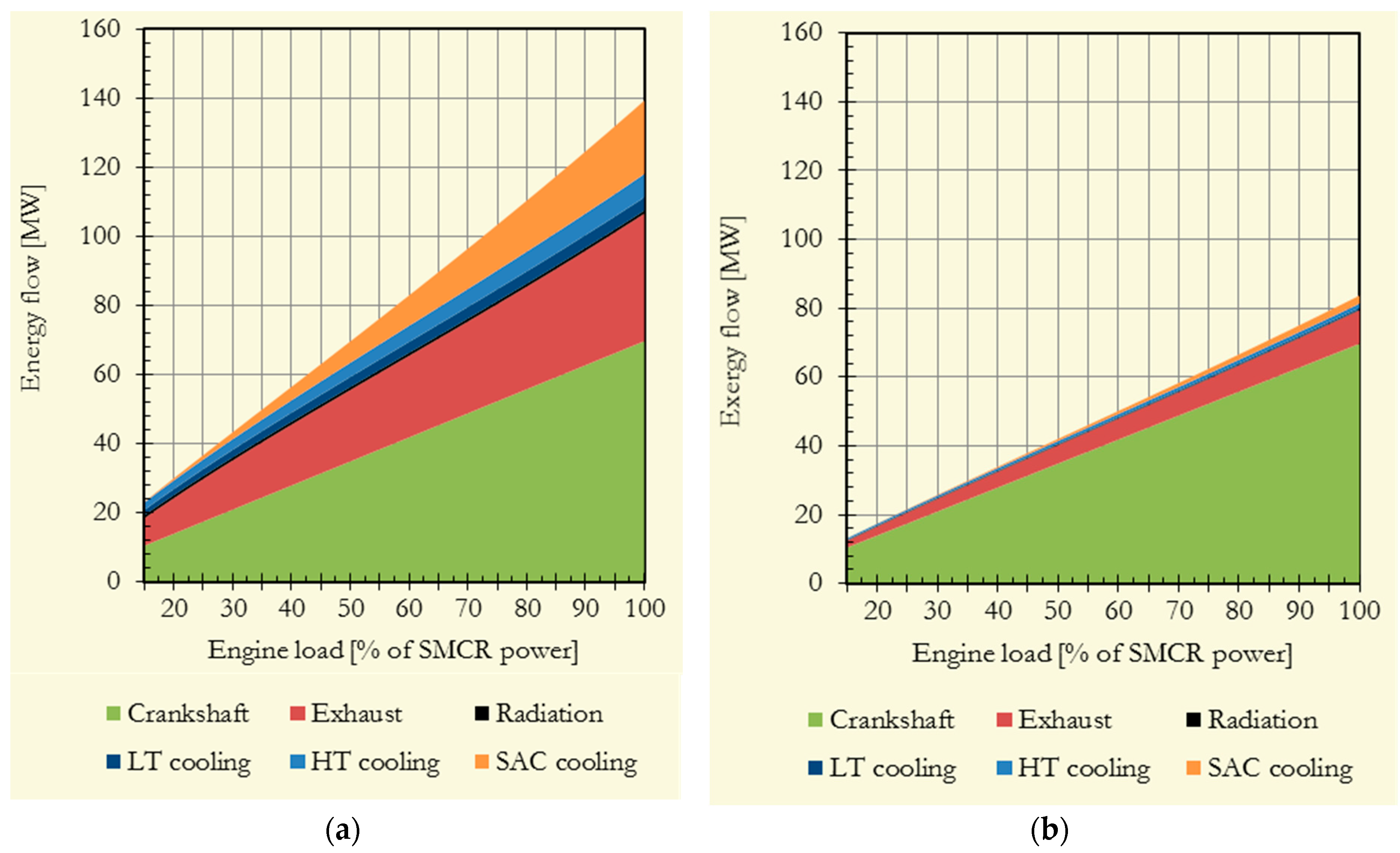
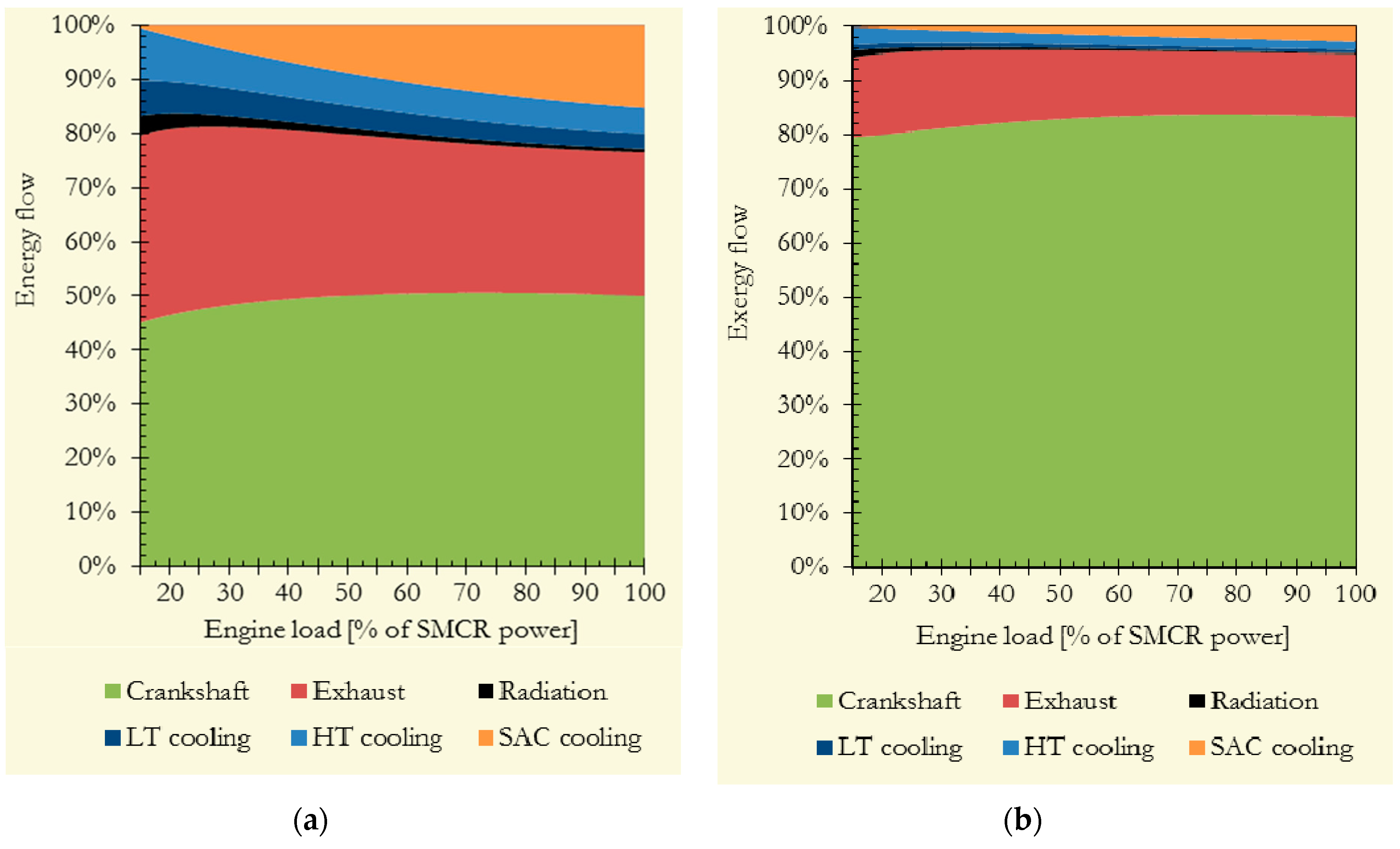
4.1. Engine Energetic and Exergetic Balance

An exergetic analysis has been carried out for the engine. The energetic and exergetic balance of its output power when operating at 70% load are presented in

Table 2. Energetic and exergetic content of the engine output power (70% load).

	Energy (MW)	Exergy (MW)	Ratio * (%)
Mechanical power	48.80	48.80	100.00
Exhaust thermal power	26.62	6.73	25.30
Scavenge air cooler thermal power	11.64	1.14	9.83
High temperature engine cooling thermal power	5.25	0.99	18.87
Low temperature engine cooling thermal power	3.36	0.38	11.43
Radiation	0.85	0.17	19.82
Total	96.53	58.21	60.31

* Exergy content over energy content.

.

Table 2 clearly illustrates the difference between energy and exergy. Considering the “Mechanical power” line, one observes that mechanical shaft has the same energy and exergy content. That is of course in accordance with theory. However, considering now the other lines of the table, one observes that energy and exergy content now differ. Thermal exhaust power, for example, has an energy content of 26.62 MW and an exergy content of 6.73 MW. This means that only 25.30% of this thermal power could be converted into mechanical power if an ideal Carnot machine were used. Hence, 74.70% of this exhaust power is anergy and doomed to stay as thermal power. The exergy content ratio, which is the ratio between the exergy and energy contents of a thermal fluid, depends on its temperature. The higher the temperature, the higher the ratio. In the end, the total exergy content of the engine climbs to 58.21 MW, which represents 60.31% of the total input power (mainly composed of the fuel chemical power). 48.8 MW are directly converted into mechanical work, and 9.41 MW hence remain to be converted. If these 9.41 MW of exergy were converted to work, the engine would have a brake specific fuel consumption (BSFC) of only 136 g/kWh, which is 16% less than current value.

The energetic and exergetic balance of the engine over the complete propeller curve are presented in Figure 3 and Figure 4. Figure 3a shows how all energy outputs increase with engine load. The Figure 4a shows how the energy distribution changes with engine load. If the mechanical part stays roughly constant, all other energy outputs, except SAC cooling, have their distribution reduced with load. The predominance of exhaust heat among “waste” energies is nevertheless clear. Figure 3b, using the same scale as the first one, clearly illustrates how most “waste” energies are mainly composed of anergy. Their exergy content is relatively small due to low output temperatures. Nevertheless, Figure 4b shows that mechanical energy represents “only” approximately 82% of the total exergy output and that 18% remain to be saved. These proportions are roughly constant along the propeller curve. Exhaust gases represent the major part of these remaining 18%.

The next section will explain how this waste exergy is either lost or destroyed and how it could be saved or even increased.

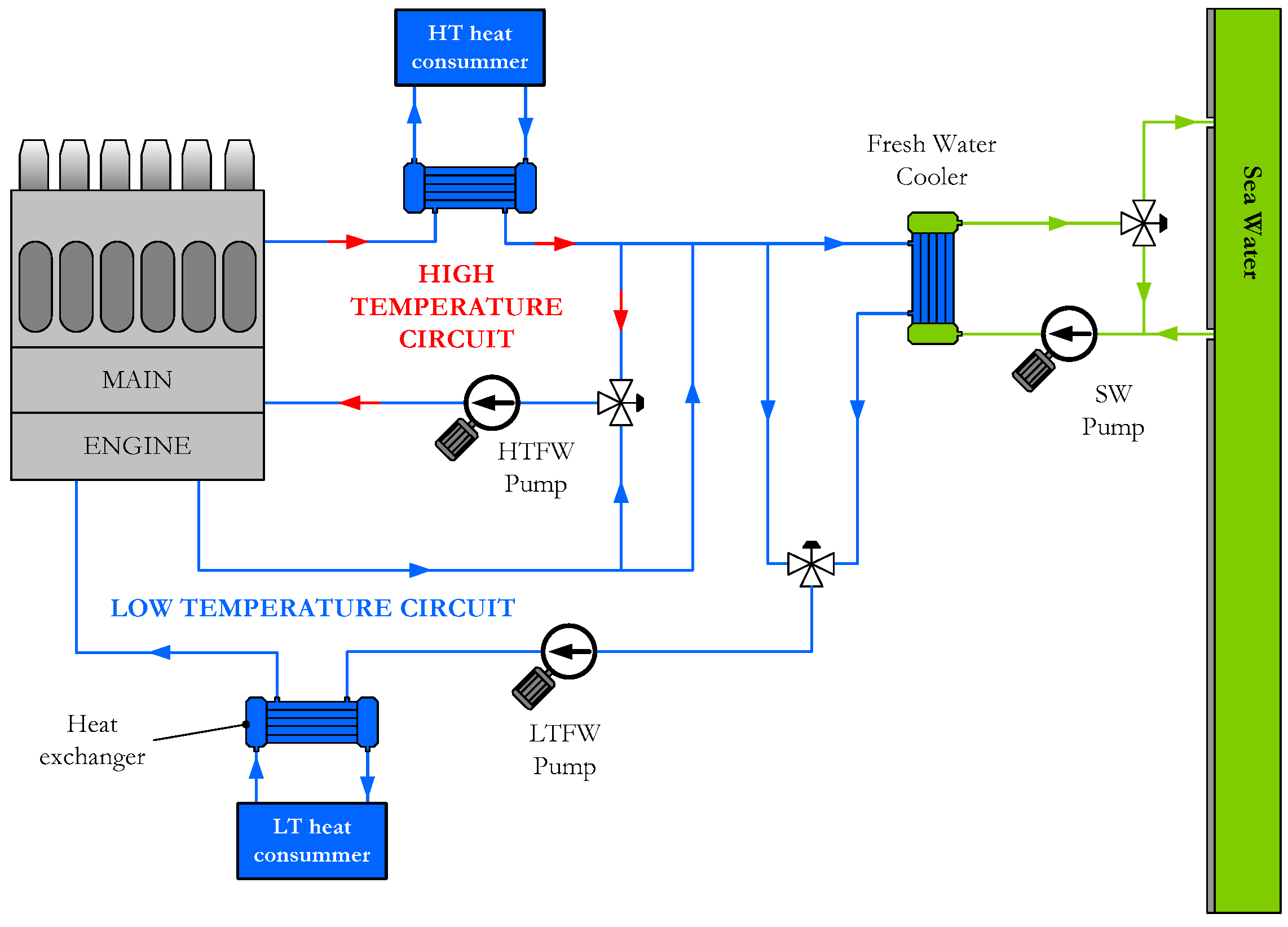
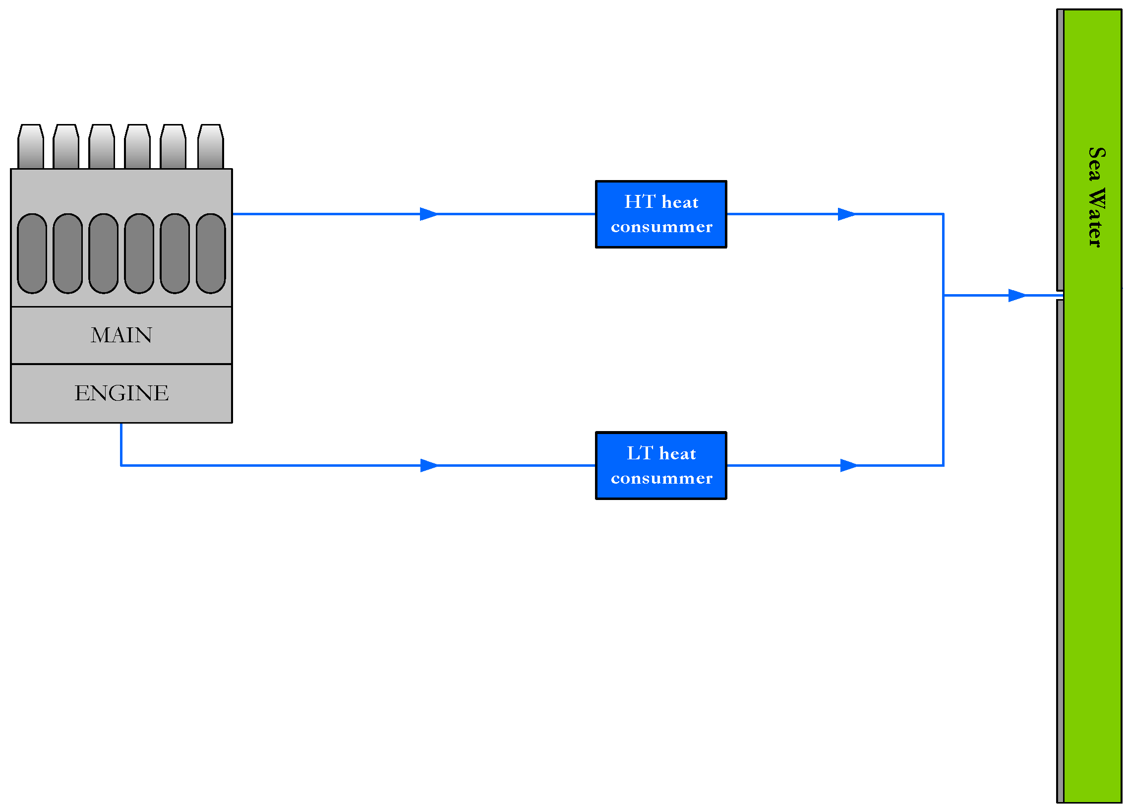
4.2. Engine Cooling and Exhaust Circuit: Energetic and Exergetic Balance

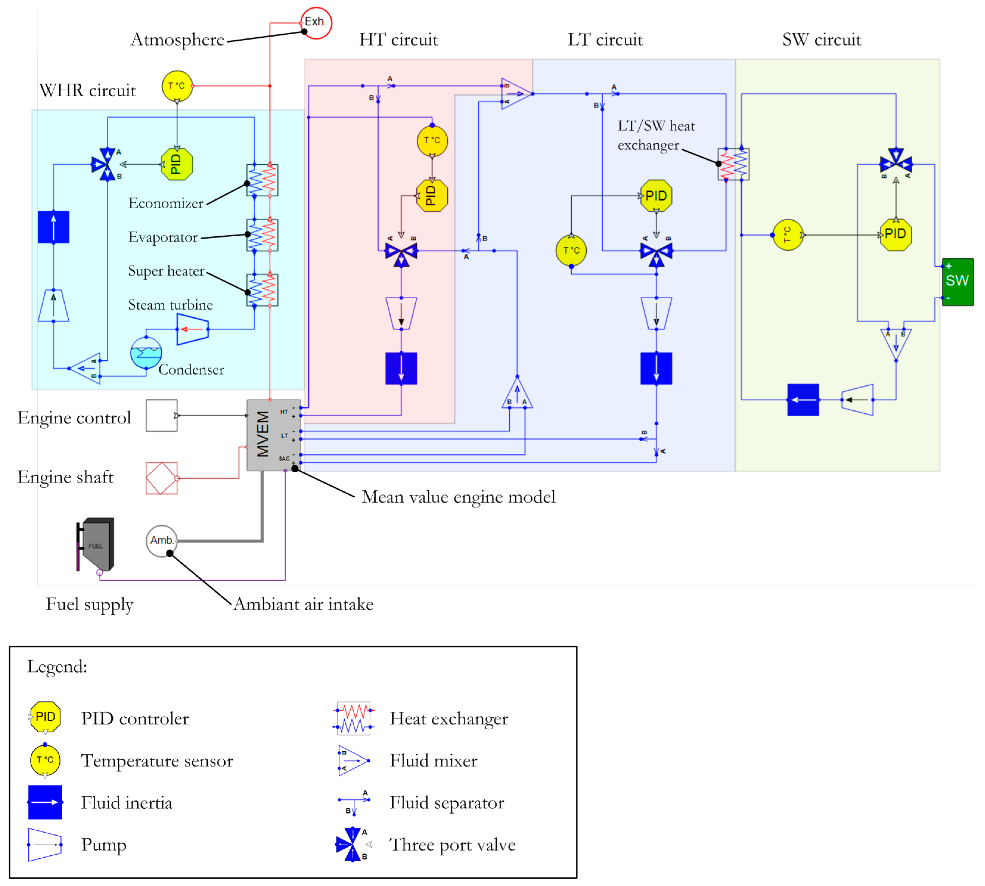
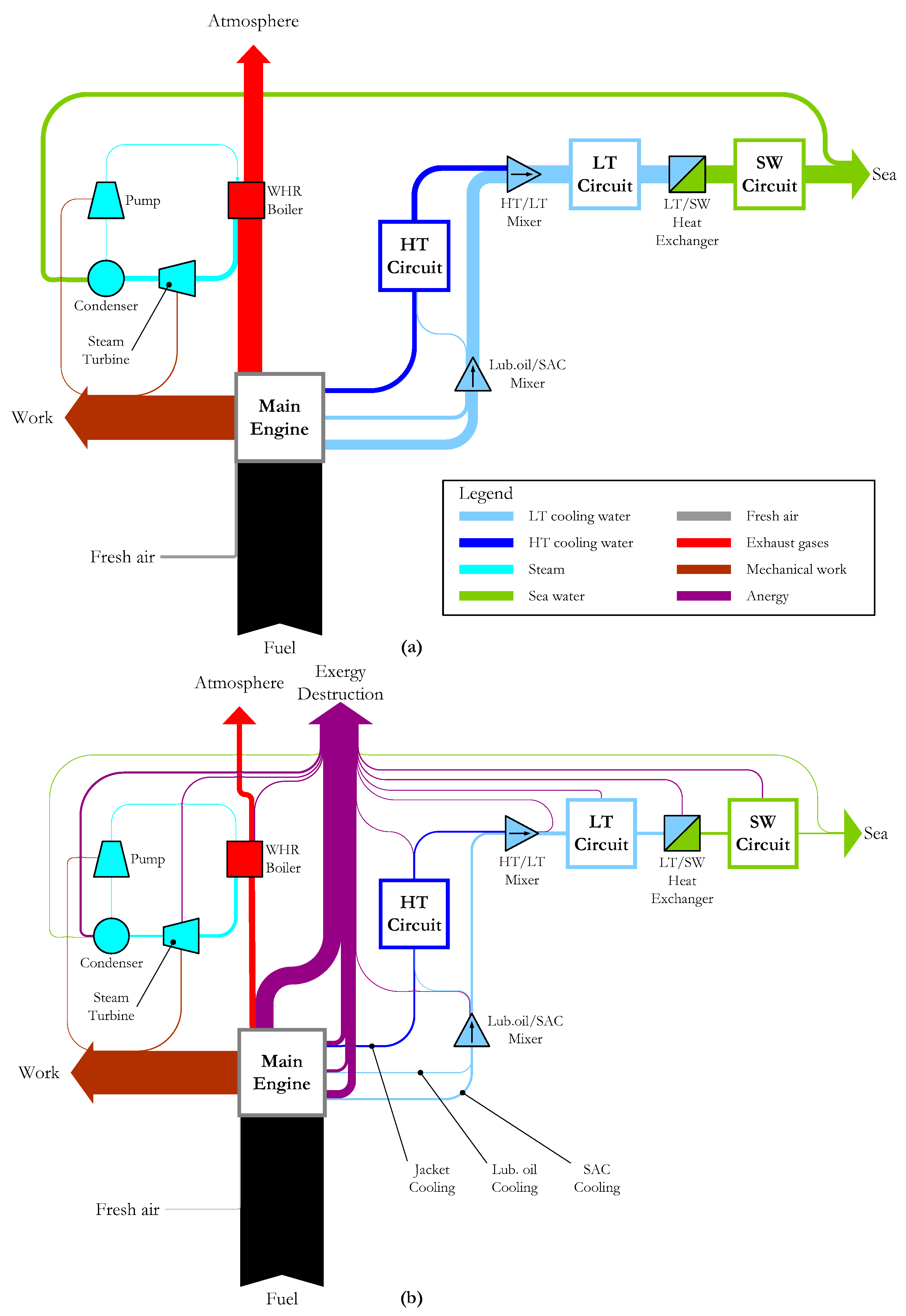
In this section, the engine is now represented with its cooling and exhaust circuits. The structure and the values of the circuits are based on a theoretical ship whose purpose is to illustrate the strengths and possibilities of the exergy analysis.

4.2.1. Presentation

The SEECAT diagram of the engine and its cooling and WHR circuit is represented in Figure 5. The engine is symbolised by the grey rectangle with “MVEM” written in it (for more details on this model see [22]). In the top left corner, the exhaust circuit and WHR system are represented. Distilled water is brought up to 22 bar by a pump and sent to the economizer and evaporator where it turns into steam (8 bar). This steam is then overheated (212 °C) in the superheater and expanded in the turbine where it produces work. It finally goes to the condenser and back to the pump. A three-port valve regulation controls the water flow in the WHR boiler to avoid exhaust gases cooling down under 170 °C (under 140 °C the sulfuric acid contained in the exhaust gases could condensate and corrode exhaust pipes). Everything on the right side of the engine represents the engine cooling system. The light red zone represents the high temperature fresh water cooling circuit; the light blue zone represents the low temperature fresh water cooling circuit and the green zone represents the sea water cooling circuit. The HT circuit cools down the engine jacket. A three-port valve controls the engine output temperature and maintains it at around 80 °C. The HT circuit is cooled down by the LT circuit, which itself cools down the engine lubrication oil system and the scavenge air cooler. The temperature in the LT circuit is regulated by a three-port valve, the temperature set point is traditionally around 36 °C. The LT is finally cooled down by the sea water circuit whose temperature is also regulated by a three-port valve to a temperature around 25 °C.

If not mentioned otherwise, the simulation is run with the parameters in

Table 3. Standard simulation parameters.

Standard Conditions	Value
Atmospheric pressure:	1 bar
Air temperature:	25 °C
Sea water temperature:	10 °C
Exergy temperature:	10 °C
Reference temperature:	0 °C
High temperature engine cooling circuit regulation temperature:	80 °C
Low temperature engine cooling circuit regulation temperature:	36 °C
Sea water cooling circuit regulation temperature:	25 °C

.

In this table, the exergy temperature represents the lower of the two environment temperatures—in this case, the sea water temperature. The reference temperature represents the temperature used for enthalpy, entropy, and thermal power calculations. Enthalpy, entropy, and thermal power of a fluid are considered null at reference temperature.

4.2.2. Simulation Results

A simulation was run with the engine load at 70%. In the previous section, the engine exergy balance was presented. It was found that “waste” energy contained 9254 kW of exergy:

• 6734 kW in the exhaust gases;
• 1144 kW in the LT circuit due to SAC cooling;
• 991 kW in the HT circuit due to engine jacket cooling; and
• 385 kW in the LT circuit due to engine lubrication oil cooling.

In most cases, this exergy is not converted into work and is hence either destroyed or lost.

Table 4. Energy and exergy flows of the engine with its cooling and exhaust systems [kW].

	${\dot{H}}_{in}$	${\dot{H}}_{out}$	$\Delta \dot{H}$	$\dot{W}$	$\dot{E}{x}_{in}$	$\dot{E}{x}_{out}$	$\dot{E}{x}_{dest}$	$\dot{E}{x}_{loss}$	$\dot{E}{x}_{gain}$
HT cooling circuit:
Jacket cooling	44,986	50,237	5251	-	3686	4677	-	-	991
Pump	44,951	44,986	34	34	3677	3706	−5	-	34
Pressure drop	44,986	44,986	-	-	3706	3686	−20	-	-
HT-LT 3-port valve	44,951	44,951	-	-	3857	3677	−180	-	-
HT-LT mixer	93,773	93,773	-	-	4587	4361	−227	-	-
LT cooling circuit:
Engine lub. oil cool.	26,904	31,037	4133	-	837	1222	-	-	385
SAC cooling	45,809	57,451	11,642	-	1425	2570	-	-	1144
LT-SAC mixer	88,488	88,488	-	-	3781	3770	−11	-	-
Pump	72,501	72,713	213	213	2234	2381	−65	-	213
Pressure drop	72,713	72,713	-	-	2381	2262	−119	-	-
Three port valve	72,501	72,501	-	-	2583	2234	−349	-	-
LT-SW exchanger	112,256	112,256	-	-	3128	2695	−433	-	-
SW circuit:
Pump	66,009	66,271	262	262	977	1134	−105	-	262
Pressure drop	66,271	66,271	-	-	1134	990	−144	-	-
Mixer	26,635	26,635	-	-	1491	977	−514	-	-
SW	30,944	9410	−21,534	-	825	-	-	−825	-
Exhaust circuit:
Engine exhaust	-	26,618	26,618	-	-	6734	-	-	6734
WHR boiler	26,917	26,917	-	-	6747	6137	−610	-	-
Power turbine	5734	5212	−522	-522	1842	1151	−170	-	−522
Condenser	5212	293	−4919	-	1151	9	−1142	-	-
Mixer	293	293	-	-	9	9	-	-	-
Pump	293	299	5	5	9	13	−1	-	5
Atmosphere	21,183	-	−21,183	-	4295	-	-	−4295	-

lists all energy and exergy flows in and out of the main components of the engine cooling and exhaust circuits. This table makes it possible to track down exergy and find out where it is lost or destroyed. The Sankey diagrams, where are flow diagrams in which the width of each flow arrow is proportional to the actual flow value, in Figure 6 are based on the same results and represent the net flows of energy and exergy. Comparing the two diagrams highlights the average low quality of energy and clearly indicates the sources of irreversibilities.

In the cooling circuits, exergy is provided by the engine and the pumps. The exergy gain brought by the pumps is almost entirely destroyed by the pressure drops inside the circuit. Concerning the exergy provided by the engine cooling, it is eventually entirely destroyed or lost. The exergy gains on the cooling circuits total 3028 kW. Two thousand two hundred three kilowatts are destroyed in the pressure drops, heat exchangers, three-port valves, and fluid mixers. It is interesting to notice that heat exchangers, three-port valves, and fluid mixers have perfect energy efficiencies: The heat flowing in is entirely transferred to the output. As for the fluid mixers and three-port valves, the process of mixing fluids—for instance, a hotter one with a colder one—is known to be highly irreversible. Concerning heat exchangers, exergy can be conserved provided there is perfect effectiveness, equal mass flow, and equal heat capacity. These conditions are of course ideal and present moreover no industrial interest. In practice, heat exchangers are always sources of irreversibilities and hence destroy exergy. Concerning pressure drop, the exergy destruction is due to the friction between the fluid and the pipes. Finally, friction, heat exchange and fluid mixing are responsible for the entire exergy destruction in the cooling circuits. The remaining 825 kW of exergy are lost in the sea but could be saved.

The exhaust circuit is where most of the exergy lies: 6734 kW released by the engine. It represents 71.5% of the waste exergy produced by the engine, whereas it contains “only” 55.8% of the waste energy. This clearly indicates where the priority lies. It is a well-known practice to add a waste heat recovery boiler to the exhaust circuit in order to produce steam. However, this steam is not always used to produce work and is often used only for heating and cleaning purposes, which is a total destruction of exergy. Adding a power turbine will help save part of this exergy. In the simulation made, 2 kg/s (7200 t/h) of steam at 8 bar are produced by the WHR boiler and expanded in the turbine. The turbine, which has an isentropic efficiency of 70%, then produces 522 kW of work for 691 kW of exergy consumed. The rest of the exergy is either destroyed or lost. The condenser destroys up to 1142 kW, the boiler heat exchangers destroy 610 kW, and 4295 kW are lost in the atmosphere.

The relative importance of the condenser in the destruction of exergy is contrary to the conclusions of Rosen [15]. Rosen had shown that condensers, even if they dissipated a lot of energy, did not destroy much exergy as the energy flow entering the condenser was of poor quality (low pressure and low temperature). The conclusion nevertheless applied to thermal power plants where the steam turbines operate at a very high pressure and temperature (typically 160 bar and 540 °C). In such conditions, turbines are able to operate a greater enthalpy variation and hence send the fluid to the condenser with less exergy. However, in any case, the exergy destruction in the condenser is not the “responsibility” of the condenser but rather the responsibility of the rest of the circuit.

Concerning the exergy lost in the atmosphere, it has already been said that the WHR system can be regulated to stop exhaust gases cooling down to below 150 °C, thus avoiding the condensation of sulfuric acid. If exhaust gases could be cooled down to lower temperatures, it would allow more steam production at higher temperatures and hence more exergy saving.

In the end, the WHR boiler and turbine system have an exergetic efficiency of 7.68%; that is to say, 7.68% of the exergy entering the system is converted into work. This small figure indicates that the system is far from ideal and that there is a considerable scope for improvements, which is, from a certain perspective, very encouraging. It means that there is no theoretical limit to a big increase in work production. Traditional steam turbine cycles have higher exergy efficiency (30%–60% range). This difference is mainly due to the lack (in the WHR boiler case) of multiple high-end turbines (high and low pressure), lack of reheating steam intakes, and lower steam temperature and pressure (8 bar and 212 °C versus 160 bar and 540 °C). Nevertheless, there are, as mentioned above, some technological limitations. If the temperature of 150 °C for exhaust gases was an absolute technological limitation (which is not the case by the way), it would be possible to define a new concept (similar to exergy or the post-combustion exergy efficiency defined in Section 2) that would measure the maximum work producible given this temperature limitation. This work would be calculated using a Carnot machine working between the fluid temperature and the temperature limitation (instead of the environment temperature as in exergy). In the present case, this work would be:

$$\begin{gathered} {\dot{W}}_{150 °C}={\dot{Q}}_{exhaust}·\left(1-\frac{T_{limitation}}{T_{exhaust}}\right) \\ =26618\text{ kW}·\left(1-\frac{150°\mathrm{C}+273.15}{223°\mathrm{C}+273.15}\right) \\ =3916\text{ kW} \end{gathered}$$

(22)

This means that if ship designers do not want to cool down exhaust gases under 150 °C, there is still 3916 kW of energy convertible into work. Of course, a new efficiency could be associated to this new concept, which would measure the ratio between the work actually achieved and the best theoretical work achievable given the temperature limitation. In this case, this efficiency would be of (522−5) kW/3916 kW = 13.2%. The figure still indicates a great potential for exergy saving.

5. Energy Performance Improvements

This section presents a set of solutions for energy performance improvements. Some of these solutions are “old” ones that have already been proposed and tested in other fields, others are recent ones just emerging and some are new. As mentioned previously, modern ships already meet their needs in thermal power thanks to energy saving. Today, new developments should focus on exergy saving. The solutions presented in this section are theoretical solutions that “work on paper”. Some of these solutions might not be economically interesting or comply with regulations. Others might be opposed to “traditional construction rules” or not even be technically feasible. It is nevertheless the role of engineers and researchers to sometimes emancipate themselves from these limitations and imagine new and bold solutions. Restarting from scratch is often salutary, and for complex problems requesting holistic approaches such as energy efficiency it is almost essential.

The solutions proposed in this section are divided in three parts: design, retrofit, and operation.

5.1. Design

Diesel engines are traditionally seen as work producers. This should no longer be the basic paradigm. They should at least be seen as work and heat producers or better as exergy and anergy producers. To that extent, engine design should focus on maximizing the production of exergy.

Today, engine cooling thermal powers have poor exergy content. The only way to increase their exergy content is to increase the engine cooling temperatures. Engines are cooled down to limit material fatigue and guarantee good lubrication (lubrication oils work best at a certain temperature). However, if the jacket cooling water is maintained at temperatures around 80 °C, this also serves to avoid evaporation. If engines were cooled down by thermal oil, the engine could be kept at a higher temperatures without risking evaporation. In the case of the engine, if it was cooled down by oil at 110 °C instead of water at 80 °C, the exergy production of the HT cooling circuit would increase from 991 kW up to 1370 kW. In the same way, if new lubrication oils working best at higher temperatures were used, the exergy production could be significantly increased. For example, with lubrication oil working at 80 °C instead of 36 °C, the exergy production of the LT cooling circuit would increase from 385 kW up to 820 kW. Applying the same logic to scavenge air cooling will not be necessarily advantageous. Increasing the temperature of the SAC cooling would mean increasing the cylinder air input temperature, which would degrade the engine volumetric efficiency. Finding an optimum balance between exergy production and engine efficiency would be an interesting study to carry out. Finally, the same logic could also be applied to the sea water cooling circuit. The temperature of the sea water cooling circuit is regulated to avoid salt precipitation that fouls the heat exchanger. This precipitation occurs around 35 °C. It could be avoided by using another fluid for cooling such as the fuel in fuel tankers. It could also be, not avoided, but ignored if the heat exchange between the LT circuit and sea water was not made through a heat exchanger but directly through the hull plating. In this case, the sea water circuit would be replaced by a fresh water circuit or simply deleted.

The exergy analysis of the engine and its cooling circuit has also highlighted the necessity to avoid heat exchangers and fluid mixers as much as possible. New designs requiring fewer heat exchangers and fluid mixers are preferable.

All these means of increasing exergy production and avoiding exergy destruction are only good if this exergy can be converted into work. A solution would be to use the HT and LT power to heat up a working fluid. For example, the HT circuit is often used for fresh water production thanks to distillers. However, today, reverse osmosis water production units have shown themselves to be more efficient. The HT thermal power could then be entirely used to heat up the water used in the WHR boiler. It would then serve as a “pre-economizer” instead of being cooled down by the LT circuit. The LT heat could also serve as a “pre-pre-economizer.” The WHR boiler could then increase the steam produced and its temperature, thereby increasing the work producible by the turbine. A second way of saving the cooling circuit exergy would be to use organic Rankine cycle systems (ORC) [25,26]. These systems convert heat into work in a similar way as the WHR boiler and steam turbine do, but, instead of using water, they use organic fluids (such as n-pentane or toluene). These fluids present the advantage of evaporating at lower temperatures than water (at ambient pressure), which makes ORC systems more efficient than steam cycles at low temperatures [27]. Moreover, ORC systems are often simpler than their steam equivalents as they do not always require superheaters, steam drums, or deaerators, making them easier to regulate and more compact. ORC systems have usually low energy efficiencies (< 25%) but are interesting from an exergetic point of view as they convert low-grade heat into work or electricity.

The analysis of the engine thermal and exergy balance has shown that the major part of “waste” energy was made up of exhaust heat and that exhaust heat had the highest exergy content ratio because of its high temperature. Exhaust gases are in fact the best exergy vectors, and new engine designs should try to increase even further the proportion of exhaust gases in waste energy (by mainly increasing output temperature if possible). A possible way to do that would be to insulate the engine. Research into this concept has already been carried out. The primary objective was to increase engine efficiency by reducing heat loss. Results were never conclusive in that regard, as it was observed that the heat saved by insulating the engine was mainly transferred to the exhaust gases [28]. This solution could then be successfully applied to diesel engines.

In order to save as much exergy as possible from the exhaust gases, the steam should be produced at the highest pressure possible. Fifteen bar could be feasible, as water then boils at around 200 °C. Moreover, it should be possible to cool down exhaust gases below 150 °C by using new materials that resist to sulfuric acid corrosion. This is already done in domestic condensing boilers. These two measures should allow more steam to be produced at a higher pressure and hence more work production.

5.2. Retrofit

Several of the solutions proposed above could also be used in retrofitting. However, this would certainly be more costly and complicated. A relatively interesting solution, which would be relatively easy to retrofit, is variable flow pumps. Most ships today use three-port valves for temperature regulation. This implies a fixed flow pump consuming a constant quantity of work whatever the cooling needs. Using variable flow pumps instead is a simple method to reduce this work demand and hence exergy consumption. Of course, there are many factors to consider. Fixed flow pumps are often more efficient than variable flow pumps and less expensive. The profitability of such an operation will also depend greatly on the ship’s average operational profile. Correctly assessing the possible gains is now made possible thanks to the “second law” approach.

5.3. Operation

The Carnot efficiency indicates that operating under cold environmental conditions is favorable. The concept of exergy easily explains this: As the environment temperature goes down, the enthalpy difference between the fluid in its current state and the fluid at environment temperature increases, and more work is producible. This theory is verified in practice. The engine’s manufacturer provides its data sheet for different environment temperatures and indicates a gain of almost 2 g/kWh in cold conditions (10 °C ambient air and sea) compared to ISO conditions (25 °C ambient air and sea). These gains should be added to possible gains in the exhaust WHR system. This energy gain could be taken into account when planning routes. When faced with two similar alternatives, the route presenting the lowest predicted sea and air temperature should be favored.

6. Conclusions

The first holistic energy ship model developed was circumscribed by certain limitations [11], notably the fact that it was based only on the first law of thermodynamics and can be described now as a first level approach. This new model moves up to a second level where the second law of thermodynamics, through the concept of exergy, is now taken into account. This new approach requires more detailed and complicated modeling but using it makes it possible to precisely pinpoint sources of irreversibility and potential work production. It globally provides a better understanding and a more physical representation of complex systems such as engine cooling and exhaust circuits. Additionally, it opens up a vast field of energy and exergy saving solutions, solutions that will require new models and simulations. However, to fully benefit from the exergy analysis, a new study based on real ship measurement is necessary. Moreover, this new approach also calls for a new level of modeling. Just as the exergy concept introduced physical limitations to the first law of thermodynamics, technology introduces limitations to the second law of thermodynamics (friction, finite dimensions, and material corrosion or fatigue). Taking into account these limitations is essential if one wants to correctly assess possible energy gains.

Finally, this new “fluid circuit” approach will be very useful to model, understand, and improve new systems such as HVAC and ORC systems.

References

1. International Maritime Organization. MARPOL: Articles, Protocols, Annexes, Unified Interpretations of the International Convention for the Prevention of Pollution from Ships, 1973, as Modified by the 1978 Relating Thereto, 5th ed.; International Maritime Organization: London, UK, 2011. [Google Scholar]
2. Buhaug, Ø.; Corbett, J.J.; Endresen, Ø.; Eyring, V.; Faber, J.; Hanayama, S.; Lee, D.S.; Lee, D.; Lindstad, H.; Markowska, A.Z. Second IMO GHG Study 2009; International Maritime Organization: London, UK, 2009. [Google Scholar]
3. United Nations Conference on Trade and Development. Review of Maritime Transport 2011; United Nations: New York, NY, USA, 2011. [Google Scholar]
4. Thomas, G.; O’Doherty, D.; Sterling, D.; Chin, C. Energy audit of fishing vessels. Proc. Inst. Mech. Eng. Part M J. Eng. Marit. Environ. 2010, 224, 87–101. [Google Scholar] [CrossRef]
5. Basurko, O.C.; Gabiña, G.; Uriondo, Z. Energy performance of fishing vessels and potential savings. J. Clean. Prod. 2013, 54, 30–40. [Google Scholar] [CrossRef]
6. Emilio, N.; Gabriele, B.; Antonello, S. An Energy Audit tool for increasing fishing efficiency. In Proceedings of the 2nd International Symposium on Fishing Vessel Energy Efficiency E-Fishing, Vigo, Spain, 22–24 May 2012.
7. Rakopoulos, C.D.; Giakoumis, E.G. Review of thermodynamic diesel engine simulations under transient operating conditions. SAE 2006 Trans J. Engines 2006. [Google Scholar] [CrossRef]
8. Rakopoulos, C.D.; Michos, C.N.; Giakoumis, E.G. Study of the transient behavior of turbocharged diesel engines including compressor surging using a linearized quasi-steady analysis. SAE Model. SI Diesel Engines 2005, 225. [Google Scholar] [CrossRef]
9. Balaji, R.; Yaakob, O. An analysis of shipboard waste heat availability for ballast water treatment. J. Mar. Eng. Technol. 2012, 11, 15–29. [Google Scholar]
10. Baldi, F. Improving Ship Energy Efficiency through a Systems Perspective. Licentiate thesis, Chalmers University of Technology, Department of Shipping and Marine Technology, Gothenburg, Sweden, 2013. [Google Scholar]
11. Marty, P.; Corrignan, P.; Gondet, A.; Chenouard, R.; Hétet, J.-F. Modelling of energy flows and fuel consumption on board ships: Application to a large modern cruise vessel and comparison with sea monitoring data. In Proceedings of the 11th International Marine Design Conference, Glasgow, UK, 11–14 June 2012; Volume 3, pp. 545–563.
12. Modelica. Available online: https://www.modelica.org (accessed on 28 March 2016).
13. Benelmir, R.; Lallemand, A.; Feidt, M. Analyse Exergétique; Techniques de l’ingénieur: Paris, France, 2002. (In French) [Google Scholar]
14. Dincer, I.; Rosen, M.A. Exergy: Energy, Environment and Sustainable Development; Elsevier: Philadelphia, PA, USA, 2007. [Google Scholar]
15. Rosen, M.A. Energy- and exergy-based comparison of coal-fired and nuclear steam power plants. Exergy Int. J. 2001, 3, 180–192. [Google Scholar] [CrossRef]
16. Koroneos, C.; Haritakis, I.; Michaloglou, K.; Moussiopoulos, N. Exergy Analysis for Power Plant Alternative Designs, Part I. Energy Sources 2004, 26, 1277–1285. [Google Scholar] [CrossRef]
17. Baldi, F.; Ahlgren, F.; Nguyen, T.-V.; Gabrielii, C.; Andersson, K. Energy and exergy analysis of a cruise ship. In Proceedings of the 28th International Conference on Efficiency, Cost, Optimization, Simulation and Environmental Impact of Eeergy Systems, Pau, France, 29 June–3 July 2015.
18. Fritzson, P. Principles of Object-Oriented Modeling and Simulation with Modelica 2.1; John Wiley & Sons: Hoboken, NJ, USA, 2004. [Google Scholar]
19. Keenan, J.H.; Kaye, J. Gas Tables: Thermodynamic Properties of Air Products of Combustion and Component Gases Comprehensives Flow Functions; John Wiley and Sons: New York, NY, USA, 1948. [Google Scholar]
20. Wagner, W.; Copper, J.R.; Dittmann, A.; Kijima, H.J.; Kruse, A.; Mares, R.; Oguchi, K.; Sato, H.; Stocker, I.; Sifner, O.; et al. The IAPWS Industrial Formulation 1997 for the Thermodynamic Properties of Water and Steam. J. Eng. Gas Turbines Power 2000, 122, 150–184. [Google Scholar]
21. Hendricks, E. Mean Value Modelling of Large Turbocharged Two-Stroke Diesel Engines; SAE Technical Paper 890564; SAE International: Warrendale, PA, USA, 1989. [Google Scholar]
22. Marty, P.; Corrignan, P.; Hétet, J.-F. Development of a Marine Diesel Engine Mean-Value Model for Holistic Ship Energy Modelling. In Proceedings of the COFRET’14—COlloque FRancophone en Énergie, Environnement, Économie et Thermodynamique, Paris, France, 23–25 April 2014; pp. 341–352.
23. Aljundi, I.H. Energy and exergy analysis of a steam power plant in Jordan. Appl. Therm. Eng. 2009, 29, 324–328. [Google Scholar] [CrossRef]
24. Borel, L.; Favrat, D. Thermodynamique et Énergétique; PPUR: Lausanne, Switzerland, 2005. (In French) [Google Scholar]
25. Larsen, U.; Pierobon, L.; Haglind, F.; Gabrielii, C. Design and optimisation of organic Rankine cycles for waste heat recovery in marine applications using the principles of natural selection. Energy 2013, 55, 803–812. [Google Scholar] [CrossRef] [Green Version]
26. Shu, G.; Liang, Y.; Wei, H.; Tian, H.; Zhao, J.; Liu, L. A review of waste heat recovery on two-stroke IC engine aboard ships. Renew. Sustain. Energy Rev. 2013, 19, 385–401. [Google Scholar] [CrossRef]
27. Suárez de la Fuente, S.; Greig, A.R. Making shipping greener: ORC modeling under realistic operative conditions. In Proceedings of the Low Carbon Shipping Conference, London, UK, 9–10 September 2013.
28. Descombes, G.; Maroteaux, F.; Feidt, M. Study of the interaction between mechanical energy and heat exchanges applied to IC engines. Appl. Therm. Eng. 2003, 23, 2061–2078. [Google Scholar] [CrossRef]
Figure 1. Schematic representation of an engine cooling system under the new “second law” approach.
Entropy 18 00127 g001
Figure 2. Schematic representation of an engine cooling system under the previous “first law” approach.
Entropy 18 00127 g002
Figure 3. (a) Absolute output energy balance of the engine. (b) Absolute output exergy balance of the engine.
Entropy 18 00127 g003
Figure 4. (a) Relative output energy balance of the engine. (b) Relative output exergy balance of the engine.
Entropy 18 00127 g004
Figure 5. SEECAT model of the engine and its cooling and WHR circuit.
Entropy 18 00127 g005
Figure 6. Energy (a) and exergy (b) Sankey diagrams of the engine with its cooling and exhaust circuits.
Entropy 18 00127 g006