
Quantum Errors and Disturbances: Response to Busch, Lahti and Werner

Centre for Engineered Quantum Systems, School of Physics, The University of Sydney, Sydney, NSW 2006, Australia
Entropy 2016, 18(5), 174; https://0-doi-org.brum.beds.ac.uk/10.3390/e18050174
Submission received: 27 February 2016
/
Revised: 25 April 2016
/
Accepted: 28 April 2016
/
Published: 6 May 2016
(This article belongs to the Special Issue Quantum Information and Communication: From Foundations to Applications)
Abstract
:Busch, Lahti and Werner (BLW) have recently criticized the operator approach to the description of quantum errors and disturbances. Their criticisms are justified to the extent that the physical meaning of the operator definitions has not hitherto been adequately explained. We rectify that omission. We then examine BLW’s criticisms in the light of our analysis. We argue that, although the BLW approach favour (based on the Wasserstein two-deviation) has its uses, there are important physical situations where an operator approach is preferable. We also discuss the reason why the error-disturbance relation is still giving rise to controversies almost a century after Heisenberg first stated his microscope argument. We argue that the source of the difficulties is the problem of interpretation, which is not so wholly disconnected from experimental practicalities as is sometimes supposed.
PACS:
03.65.Ta1. Introduction
The error-disturbance principle remains highly controversial almost a century after Heisenberg wrote the paper [1], which originally suggested it. It is remarkable that this should be so, since the disagreements concern what is arguably the most fundamental concept of all, not only in physics, but in empirical science generally: namely, the concept of measurement accuracy. Measuring instruments are not born equal. If one did not have a way to distinguish measurements that are in some sense “good” from measurements that are in some sense “bad”, that is if one did not have what Busch et al. [2] call a “figure of merit”, one would be forced to regard all measurements as being on the same footing. There would, in fact, be no reason to prefer numbers obtained using a state-of-the-art photon counter from those obtained using the less expensive, less demanding procedure of making a blind guess. Under such conditions, empirical science would be impossible. Since physics has actually made huge advances over the last century, it is obvious that, on a practical level, experimentalists have ways to distinguish good measurements from bad. However, those practical methods are not supported by an adequate understanding at the theoretical level.
It is worth asking why, given the fundamental importance of the problem, progress has been so slow. Although it is true that the problem is technically demanding, it appears to us that the main obstacle has always been, as it continues to be, conceptual. The classical concept of error involves a comparison between the measured value and the true value, as it existed before the measurement was made. The Bell–Kochen–Specker theorem [3,4,5,6], however, requires us to abandon the idea that a measurement ascertains the pre-existing value of a specified observable (aside from cases where there is a superselection rule). This is such a radical departure from classical ideas that Bell [7] suggested that “the field would be significantly advanced by banning [the word ‘measurement’] altogether, in favour for example of the word ‘experiment’ ”. The question then arises: once the classical concept of measurement has gone up in smoke, what, if anything, is left of the classical concept of measurement accuracy? It will be seen that this is a special case of the more general question, which lies at the heart of all of the disputes about quantum foundations: once the classical concept of measurement has gone up in smoke, what, if anything, is left of the classical concept of empirically-accessible reality? The problem is consequently of a rather peculiar kind. Physics encompasses an enormous spectrum of problems, ranging from nuts-and-bolts problems, such as measuring a length precisely, to deep philosophical questions. The error-disturbance principle is unusual because it directly connects the two ends of the spectrum. On the one hand, it has, as we stressed above, an immediate, down-to-earth practical relevance. On the other hand, we would argue that one of the factors obstructing progress, the reason almost half a century elapsed before people started to come seriously to grips with the problem, was the obscurities of the Copenhagen interpretation. It thus provides a riposte to the suggestion that the interpretational issues are practically unimportant.
Although the connections with the interpretation problem are not the main point of this paper, they are part of the underlying motivation. It is therefore appropriate to say something about them in this introductory section (we shall give a more detailed discussion in a subsequent publication). Let us begin by observing that Heisenberg himself did not propose or even conjecture an error-disturbance principle. He did, of course, construct his famous microscope argument [1,8], which has suggested to many that he had in mind such a principle. However, that is based on a misunderstanding of the point of the microscope argument (that is, what Heisenberg saw as the point). That point emerges most clearly in Von Neumann’s account [9], where it is made completely explicit that the function of the microscope argument is to give intuitive support to the inequality proved by Kennard [10] and Weyl [11] (the latter attributing the result to Pauli) and to its subsequent generalization by Robertson [12] and Schrödinger [13]. In his 1927 paper [1], Heisenberg was less explicit. At the time he wrote the paper, the Kennard–Pauli–Weyl proof was yet to come, and perhaps for that reason, he gave the microscope argument pride of place. However, he was using it to support his original prototype for the uncertainty principle, namely the order of magnitude estimate , where , are the standard deviations of the p, q probability distributions scaled by a factor . There is no indication that he envisaged, in addition to this statement, an entirely different error-disturbance principle.
Nevertheless, although Heisenberg did not in fact propose an error-disturbance principle, one may feel that he should have done so, for it is strongly suggested by the considerations in his 1927 paper (to that extent, we agree with Busch et al. [14], that it is “latent” in what he says). Reflecting on the microscope experiment, it seems intuitively evident that the measurement of position really is (in some sense) less than perfectly accurate and that the electron really will (in some sense) be disturbed by the photon. The situation seems to be crying out for proper quantum mechanical analysis. Yet, it evidently did not seem that way to Heisenberg; nor, apparently, did it seem that way to most other people before the 1960s. During the period between 1927 and the 1965 paper of Arthurs and Kelly [15] which gave the first explicit model for a joint measurement of position and momentum, one finds various paraphrases and elaborations of the statements in Heisenberg’s original paper, but we are not aware of any clear statement of the error-disturbance principle conceived of as a proposition distinct from the Kennard–Pauli–Weyl inequality or any recognition of the fact that a quantum mechanical definition of measurement accuracy is needed. The question arises: Why is it that Heisenberg and so many others failed to draw what seems to most people now the obvious conclusion from his uncertainty paper? The answer, we suggest, is that their understanding was obstructed by one of the features of the Copenhagen interpretation.
In the words of Bell [16], the Copenhagen interpretation divides the world “into speakable apparatus ...that we can talk about ...and unspeakable quantum system that we can not talk about” (ellipses in the original). Of course, the Copenhagen interpretation is not a sharply defined entity [17,18,19]). However, it appears to us that Bell’s one-sentence summary does identify an idea that, in one form or another, is common to all the many variants. This idea has been hard to maintain since the 1970s, when it was realized, in connection with the problem of gravity-wave detection, that the error-disturbance principle is relevant to highly accurate measurements of a macroscopic oscillator [20,21]. Such an oscillator is just as speakable as any other piece of laboratory apparatus; yet, at the same time, we need to analyse its behaviour quantum mechanically. However, in the early days of quantum mechanics, the unspeakability of quantum systems was accepted by almost everyone. Thinking of the quantum world as ineffable and beyond the reach of thought [22], forgetting that the quantum world is the one in front of our noses, encouraged the perception that quantum mechanical measurements are so utterly different from classical ones that no points of contact with classical concepts are possible. In particular, it encouraged the assumption that the classical concept of error cannot carry over to quantum mechanics in any shape or form. This, we would suggest, is why Heisenberg did not follow through on what now seems the obvious implication of his microscope argument and formulate an error-disturbance principle. He did not do so because he rejected the very idea of a quantum error or a quantum disturbance.
Corresponding to the idea that there are two different worlds, speakable and unspeakable, there is a widespread assumption that there are two kinds of measurement, classical and quantum. If highly accurate determinations of the centre-of-mass motion of a macroscopic object are to be treated as quantum measurements, then it is hard to see how one can consistently make such a distinction. Instead, one seems forced to the view that every measurement is a quantum measurement, measurements with a meter rule not excluded. To be sure, low precision measurements with a meter rule permit simplifying assumptions that cease to be valid as one increases the accuracy. However, that is purely a matter of practical convenience, not the signal of a fundamental difference of kind. In the case of kinematics, we continue to use the Newtonian theory when analysing low velocity motion, without taking this to mean that there is a fundamental difference of kind between the relativistic momentum of a space-ship travelling at near light speed and the Newtonian momentum of a train on the London underground. Similarly, in the case of measurements, we need a unified description.
In particular, we need a unified description of measurement errors. The statement, that the kind of sophisticated measurement on a macroscopic object that demands a quantum analysis is more accurate than a commonplace measurement with a meter rule, tacitly assumes that there is a single concept of accuracy applicable to both. Otherwise, we would not have the basis for a comparison. In the case of kinematics, the Newtonian definition of momentum is an approximation to the relativistic definition, valid for low velocities. In the same way, one would like an overarching quantum definition of error, which effectively reduces to the classical one in limiting cases. At first sight, this may seem impossible, since quantum mechanics requires us to drop the assumption that a measurement ascertains the pre-existing value of a specified observable. However, on further reflection, it will be seen that even on classical assumptions, one is never able to directly compare the measured value with the pre-existing true one. In classical physics, as in quantum physics, measured values are the only ones available. It follows that, although in classical principle the error is the difference between the measured value and the true one, in point of classical practice it must be possible to do everything using measured values only.
The purpose of this paper is to make a small beginning on the task of constructing a unified theory of measurement. We focus on Busch, Lahti and Werner’s (BLW’s) criticisms [2,23,24,25,26] of the operator approach [27,28,29,30,31] to the description of quantum errors and disturbances. Their criticisms raise some issues that are highly relevant to the above discussion and that need to be settled if we hope to make progress. It should be stressed that although our conclusion is that the operator approach is more useful than BLW allow, we are far from rejecting everything they say. In particular, we completely agree with them on what is, perhaps, the most essential point, that quantum errors and disturbances need to be defined operationally. Moreover, in defending the operator approach, it is no part of our intention to impugn the distributional approach they favour. No one would say that the RMS characterization of an ordinary uncertainty is either “better” or “worse” than an entropic characterization. Rather, one has different quantitative measures, each of which has advantages and disadvantages; similarly here. The task is not to single out one particular approach as somehow canonical, but rather to achieve a clear understanding, at the basic conceptual level, of what is meant by the words “error” and “disturbance” in a quantum mechanical context and of the different ways of quantifying the concepts.
There are two versions of the operator approach (or O approach, as we will call it from now on). BLW’s criticisms are largely directed against the state-dependent version proposed by Ozawa [28,29]. However, we had previously proposed a state-independent version [27]. Both versions are relevant to our discussion. In Section 2, we compare and contrast them.
Section 3 is the core of the paper. We begin with the classical concepts of error and disturbance. We show that there are at least two ways to reformulate them in a manner that does not involve a comparison with pre-existing values. We then show that the reformulated definitions have natural quantum generalizations, which we call the D and C definitions. The D and C errors are thus candidates for the overarching concept of measurement accuracy, which, as we argued above, is necessary if one wants to construct a unified theory of measurement, in which every measurement is seen as quantum. They also have an important bearing on BLW’s criticism of the O approach. As BLW correctly observe, the O definitions are non-operational. However, the D and C definitions are operational. Moreover, the O quantities are upper bounds on the corresponding D and C quantities. This gives indirect operational meaning to the O quantities. Specifically, it means that if one of the O quantities is small, then there are at least two well-defined operational senses in which the measurement is accurate or non-disturbing. The situation when an O quantity is large is more problematic. In the state-independent case, it is possible that the smallness of the O error/disturbance is both necessary and sufficient for the measurement to be accurate/non-disturbing in a well-defined operational sense. However, we have not been able to prove this.
In Section 4, we analyse BLW’s objections to the O approach in light of the foregoing. BLW contrast the operator approach with what they call a distributional approach. It is to be observed, however, that the D and C quantities are also defined distributionally. Since the O quantities owe their physical meaning to their connection with the D and C quantities, it follows that the O quantities are indirectly distributional. In short, the problem is not to decide between a distributional approach and some other, completely different approach. Rather, it is to decide between two different kinds of distributional approaches. As with all such questions, the answer is relative to the situation of interest. We show that there is at least one important class of physical problems for the which the D error and, by extension, the O error are clearly more appropriate than the definition that BLW favour, based on the Wasserstein two-deviation.
2. The Operator Approach
In this section, we outline the operator characterization of quantum errors and disturbances. Our aim is purely descriptive. We justify the approach, and respond to the various criticisms that have been made of it, in subsequent sections.
Consider a classical measurement of position. Let , be the position and momentum immediately before the measurement, and let , be their values immediately after it. Let be the final value of the pointer observable. Then, the error in the measurement of position is , and the disturbance to the momentum is (classical physics does not, of course, require there to be a disturbance to the momentum, but such a disturbance is perfectly possible). On the level of formal analogy, it is natural to ask what happens if one replaces the classical variables in these expressions with the corresponding Heisenberg picture operators. Let and be the Hilbert spaces for the system and apparatus, respectively, and assume that the system + apparatus are initially in the product state , where is the density matrix of the system and is the density matrix of the apparatus. Let be the unitary operator describing the measurement interaction, let
be the position, momentum and pointer Heisenberg picture observables immediately before the measurement interaction commences, and let
be the Heisenberg picture observables immediately after the interaction has finished. Formal analogy with the classical case then suggests that we define
In Appleby [27,32,33,34] we also introduced the predictive error operator . We shall not discuss it here since it does not give rise to conceptual difficulties. We refer to (respectively, ) as the error (respectively, disturbance) operator. We then obtain a numerical characterization of the error by defining
and a numerical characterization of the disturbance by defining
We label the quantities with a superscript because, while the apparatus “ready” state is assumed to be always the same, the system state can vary. The operators , are unbounded, which means that the quantities , are not defined for every state . In the following, we will always assume that is in the set of physical states defined in the Appendix. If this is true, then, provided that is appropriately chosen, the expectation value is well defined and finite for every monomial M in , , , , , .
Of course, we have not yet justified the interpretation of and as an error and disturbance (beyond noting the formal analogy with classical physics, which, though suggestive, is clearly not sufficient to justify the proposal). We defer a proper justification to the next section and focus here on the question of whether there exists an error-disturbance relation expressible in terms of these quantities. In various special cases [15,32,33,35,36,37,38], one does indeed have
analogous to the ordinary uncertainty relation . However, as we showed in [27], it is easy to see that the inequality cannot be generally valid. In [27] we were concerned with joint measurements of x and p; however our argument also applies to single measurements of x only because any such measurement can be regarded as a joint measurement in which the momentum pointer does not interact with the system. Indeed, the example we gave was of precisely this kind. Eliminating the inessential reference to the momentum pointer we gave a simple model for the measurement process, in which the position pointer is the position of a particle having momentum and in which the measurement rotates the system particle position onto the pointer particle position, so that
Such a rotation is effected by
where
(so, if , were different components of the position of a single particle in three dimensions, would be a component of the angular momentum operator). The fact that means that . It is easy to see that . Therefore, this is a measurement for which the error is zero, while the disturbance is finite for every physical state.
Although we are mainly concerned with the error-disturbance relation in this paper, it is worth noting that exactly the same argument shows [27] that the error-error relation
for a joint measurement of position and momentum cannot be valid in general. Indeed, consider a joint measurement in which the interaction of the particle with the position pointer is described by the unitary in Equation (8), while the momentum pointer just goes along for the ride, without interacting at all. One then has and (where is the momentum pointer position). Even though the momentum is not really being measured at all, is still finite for every physical state. Therefore, inequality (10) is violated for every physical state.
The fact that inequalities (6) and (10) are not generally valid was noted by us [27] and subsequently by Ozawa [28,29,39,40,41]; in the case of (10) also by Hall [42]. We, Ozawa and Hall responded to these facts by trying to find alternative inequalities that are generally valid. However, we, on the one hand, and Ozawa and Hall, on the other, were led in different directions. We begin by describing our approach to the problem, since this came first in point of time.
The essential point will emerge most clearly if we start with the violation of inequality (10) by the measurement described by Equation (8). For this measurement, it is not simply that the product is less than for a certain subset of initial states. The product is in fact strictly zero for every possible initial state. However, it would be rash to conclude from this that the measurement is in some sense “best possible”. As we noted above, the momentum pointer does not interact with the system, which means that so far as momentum is concerned, the measurement is not only not highly accurate, it cannot properly be described as a measurement at all. It is true that is small for a certain, highly specific set of initial states. However, that is not a reason for describing the measurement as accurate. Consider the following scenario:
Alice goes to Bob’s shop and buys what Bob says is a highly accurate ammeter. However, when she gets home, she finds that the needle is stuck at the 1 amp position. When she goes back to complain, Bob is unrepentant. He insists that the meter is indeed highly accurate provided one uses it to measure a 1 amp current.
Clearly, Alice will not be satisfied with this response. No more would she be satisfied with the claim that the interaction described by Equation (8) gives a highly accurate measurement of momentum.
This example shows that the smallness of the product is not always the signature of a highly accurate joint measurement of position and momentum. Similar remarks apply to the product . Consider, for instance, a “measurement” for which is the identity, so that there is no coupling whatever between system and apparatus. Here, is zero for every possible initial state, while is always finite and sometimes small. Yet, as in the broken ammeter example, it would be an abuse of language to describe this as a measurement of position that is always non-disturbing and sometimes highly accurate.
In [27], these considerations led us to look for replacements for the products , whose smallness can unequivocally be regarded as the signature of a measurement that is in some sense “good”. In the broken ammeter example, what makes Bob’s claim absurd is the fact that an accurate classical ammeter is one for which the measured value is close to the true one, not just for one particular current, but for every current within a wide range. Applying the same principle to the quantum case suggests that we define the error by
where is the set of physical states, as defined in Appendix A. As we saw above, the smallness of for some particular is consistent with the apparatus being completely decoupled from the system, so that it is not really measuring anything. However, if is small, it means that is small for every possible state, and we clearly are entitled to say that the measurement is highly accurate (taking into account the discussion in Section 3). Similar principles apply to the concept of disturbance. Consider, for instance, the measurement described by Equation (8), which rotates onto . For this measurement, will be small for certain special choices of and . However, it will typically be large. A medical procedure would not usually be described as non-invasive merely on the grounds that it can occasionally happen that the patient escapes almost intact; similarly here. We accordingly define the disturbance to be
With these definitions, it can be shown
where we use the convention, here and elsewhere, that a product of the form counts as infinite, even if . The quantity on the left-hand side should not be confused with . It is an open question whether the latter satisfies a similar inequality.
One can also prove a universally valid version of the error-error relation for a joint measurement of position and momentum
where is defined by taking the supremum of . In [27], we gave a proof of these relations, which glossed over some questions to do with domains of definition and differentiability. A completely rigorous proof is given in Appendix A below.
The quantities , are not without interest, as we discuss below. However, they are not the appropriate definitions for a real measuring instrument. The demand that be small is the demand that be small, not only when is a wave-packet localized in the vicinity of the apparatus, but also when is a wave-packet localized on the other side of the cosmic event-horizon. Clearly, this is not a reasonable demand to make of a practical laboratory instrument, which is only designed to give accurate readings for a restricted set of input states. In [27], we accordingly proposed the following modified definitions:
where the supremum is now taken over a proper subset of the set of physical states. We took to be a set of physical states for which the mean values , lie in a rectangular region of phase space with sides , and satisfying certain additional conditions. We then proved the inequalities
where we again use the convention that a product of the form counts as infinite, even if . It will be observed that in the limit as , , we recover inequalities (13) and (14). As with inequalities (13) and (14), the proof of inequalities (17) and (18), which we gave in [27], glossed over certain details. We give a completely rigorous proof in Appendix A below, where we also take the opportunity to strengthen the statement somewhat.
In practice one might not want to make a sharp distinction between states which are in the operating range of the instrument and ones which are not. There are various ways in which definitions (15), (16) might be modified to take this into account, but that would take us beyond the scope of this paper.
Let us now turn to the approach of Ozawa [28,29,40,41] and Hall [42]. In our approach, we replaced the state-dependent definitions , with the quantities , and , and proved inequalities applying to those. Ozawa [28,29], by contrast, kept with the state-dependent definitions and showed
where , are the ordinary uncertainties in the state . He also showed that [40,41], for a joint measurement of position and momentum,
It will be observed that these relations have a similar mathematical form to our inequalities (17) and (18). Hall [42] proved a relation similar to inequality (20). Other modifications and improvements have also been proved [43,44,45].
The reader should not conclude from our earlier discussion that we have any objection to the state-dependent definitions employed by Ozawa, Hall and others. Asking whether a state-independent definition is better than a state-dependent one is like asking whether a hammer is better than a screw-driver. The answer to all such questions, concerning the suitability of a tool, is relative to the use to which it is put. The fact that Bob, in the broken ammeter example, makes an inappropriate use of it does not invalidate the idea that the classical error is the difference between the measured value and the true one. The same applies here. It is true that there exist quantum analogues of the broken ammeter—processes that do not properly count as a measurement for which the state-dependent error is small. Nevertheless, the state-dependent error has a well-defined physical meaning (as we discuss in Section 3), and this makes it a potentially useful tool. State-independent definitions, such as the ones proposed by ourselves or BLW [2,23], have the advantage that they supply what BLW call an overall figure of merit; while state-dependent definitions, if not handled with care, can lead to unreasonable conclusions. However, as Rozema et al. [46] point out, state-independent definitions have the disadvantage that they are insensitive to fine, state-dependent details, which can be important. The state-dependent error can be used to analyse those details. It is to be observed, furthermore, that the state-dependent quantities , are the limits of , as is shrunk to a single point. If one takes the view that use of , is in all circumstances inappropriate, then it is hard to see how one can avoid taking the view that the use of , is also inappropriate when is very small. Which raises the question: “Just how large has got to be in order for the use of , to be justified?” It is difficult to see how the answer can be other than arbitrary. It appears to us that such discussions are fruitless and that the solution to the quandary “state-dependent or state-independent?” is not to regard it as a quandary. Instead of making a once-and-for-all choice, we are free to use either or both, in a manner adjusted to the question of interest. We return to the points raised in this paragraph at the end of Section 4.
So far from being rivals, Ozawa’s inequalities and ours are closely related. Let be any region satisfying the condition of Theorem 4 in the Appendix. If we take the supremum on both sides of Ozawa’s inequality (19), we obtain the relation
where
This is weaker than our inequality (17) if , are large, but stronger if they and the region are small. It is probably fair to say that that an experimenter will never be committed to the proposition that the system state is precisely . The statement, that the length of a rod is , will not usually be taken to mean that the length is to infinitely many decimal places. Rather, it will be taken to mean that the length is in the interval . A similar principle applies to statements regarding the wave function. This is true even in a Bayesian approach [47], where quantum states are interpreted as gambling commitments (the fact that gambling commitments are not, in practice, expressed in terms of arbitrarily large integers means that state space has to be coarse-grained in this approach). It follows that a so-called state-dependent definition of error or disturbance is really a state-independent one for which the region is very small. If is sufficiently small one will want to use Ozawa’s inequalities, but if it is larger one will want to use ours (provided satisfies the condition of Theorem 4).
Although will, in practice, only be small for a restricted set of states, the limiting situation, when it becomes zero for all , is still conceptually important. It can be shown (Appleby [34], Ozawa [48], Busch [49]) that the condition is both necessary and sufficient for the distribution of measured values to be . No real measuring instrument could have precisely this distribution of measured values for every input state ; in particular, it cannot do so for states such that the support of is not compact (in this connection, it may be worth remarking that the x and p space wave-functions cannot both have compact support, meaning that at least one of the two distributions , must be practically unrealizable). Nevertheless, the idea that is the probability distribution for a measurement of position has played a fundamental role in physical thinking ever since Born [50,51] first proposed it (in connection with the momentum distribution). There is no problem here, provided we understand the proposal to be, not that is an operational distribution (one corresponding to an actual measurement), but that it is the canonical or target distribution to which an operational distribution may conform more or less well.
A similar result can be proved for joint measurements minimizing the product : namely, that the product is minimized if and only if the distribution of measured values is the Husimi function (Appleby [34], Werner [52], Busch et al. [14]). In Appleby [53], we extended the analysis to measurements of angular momentum and showed that a determination of spin-direction is optimal if and only if the distribution of measured values is , where is a suitably-normalized coherent state.
3. Physical Interpretation of the Operator Definitions
We now come to the problem of interpreting the quantities defined in the last section. Quantum mechanics forces us to drop the classical assumption that a measurement ascertains the pre-existing value of a specified observable [3,4,5,6]. Even if one postulates that the observable measured does have a pre-existing value, that value must typically differ from the value found by measurement. In the Bohm theory, for example, the result of a measurement of velocity is usually quite different from the postulated pre-existing velocity [54,55,56,57]. Classically, the error is usually defined in terms of the difference between the measured value and the pre-existing true one. It might consequently seem that, in abandoning the idea that measurements ascertain pre-existing values, we are obliged also to abandon the concept of experimental error (in the Introduction, we argued that that is exactly how it did seem to, for example, Heisenberg). We begin by showing that that is not the case. Specifically, we describe a classical model for which the classical error can be defined in a way that does not involve a comparison with pre-existing values. We then show that this alternative definition naturally carries over to quantum mechanics.
The example we consider is that of a one-dimensional classical gas. Let x and p be the position and momentum of a particular particle in this gas, and let be the phase space probability measure. Suppose we measure x. Let be the pointer position after the measurement. We assume that the measurement process is stochastic and is described by a transition kernel , such that the expectation value of a function is given by (see, for example, Cinlar [58])
The superscript λ is to serve as a reminder that λ is arbitrary, unlike χ, which characterizes the measurement interaction and is therefore fixed. Define
It will be seen that is the RMS difference between the measured value and the pre-existing true one when λ is concentrated on the single point . We then define the classical error by
Of course, this definition is open to the same objection as the quantity defined in the last section; namely, that it is likely to be infinite for a realistic model. However, this need not detain us, because we are not interested in the model for its own sake, but only as a conceptual bridge, which will take us from classical intuition to a reasonable quantum mechanical definition of measurement error. Now, let
be the mean and standard deviation relative to the measure λ. Then, by an application of the Cauchy–Schwartz inequality,
Thus, the classical error bounds the increase in the RMS deviation of the pointer position from the initial state mean as compared to the initial state standard deviation. Note that , are λ-dependent, but is not. The inequality is actually tight. To see this, choose a sequence , such that , and let be the measure concentrated on the point . Then
Therefore
where is the set of all phase-space probability measures. This gives us an alternative formula for the classical error.
We can derive a similar formula for the classical disturbance. Let be the momentum after the measurement and the transition kernel, such that
Define the classical disturbance by
Then, by an argument similar to the one above, we find
We are now free to throw away the ladder and take Equations (29) and (32) to be the definitions of , . These alternative definitions do not involve a direct comparison between the measured value and the pre-existing one. Consequently, they do not involve the expectation values of products of pairs of variables like and x, which, in a quantum mechanical context, become non-commuting operators. Instead, they are framed in terms of the moments of probability distributions, which are also defined in quantum mechanics. They therefore generalize. Just as we can classically, so in quantum mechanics, we can define the error and disturbance in terms of the increase in an RMS deviation from an initial state mean
where we employ the notations of the last section, together with
We may also define
We will refer to these as the D definitions (“D” for “maximal increase in the RMS deviation from the initial state mean”). They are important because they show that the Bell–Kochen–Specker theorem is not, as it might seem, an insuperable obstacle blocking the path from the original classical intuition to a satisfactory quantum generalization. On the contrary, if the concepts are appropriately formulated, there is complete continuity between classical and quantum in this regard. However, although the D definitions are valid and useful, they should not be regarded as canonical. In the first place, there are other classical definitions that also have natural quantum generalizations (as we will see in the next paragraph). In the second place, there is no reason to make classical physics the arbiter. There may be useful quantum definitions that are not the generalization of any classical concept.
We arrive at another natural generalization of classical ideas if we consider measurements on a pair of correlated particles. Suppose we have two particles with positions , and momenta , and suppose we measure . Suppose that the unitary operator describing the measurement interaction is of the form , where acts on in the product (, , being respectively the Hilbert spaces of particles A, B and the apparatus). Let be the pointer position. Classically, it would be natural to define the error to be the maximal increase in the correlation as compared to and the disturbance to be the maximal increase in the correlation as compared to . The point to notice here is that . Therefore, the classical definitions are expressed in terms of the moments of probability distributions, which are also defined quantum mechanically. They therefore generalize to
where
being the set of physical states , such that . We may also define
We refer to these quantities as the C definitions (“C” for “correlation”).
Let us now turn to the definitions in Section 2, which we will refer to as the O definitions (“O” for “operator”). The commutators and are typically non-zero, so the O quantities are typically not generalizations of the corresponding classical quantities, as Busch and co-workers have stressed [24,49]. The O quantities do, however, impose bounds on the D and C quantities, and this gives them an indirect physical interpretation. We have
from which it follows
for all . Similarly
Taking suprema, we deduce
When , these inequalities reduce to
We also have the following constraints on the relative sizes of the D and C quantities:
These inequalities mean, among other things, that the O quantities are upper bounds on the corresponding D and C quantities.
Our discussion raises some important questions. If is large, then the above inequalities are consistent with one of the O quantities being large, while the corresponding D and C quantities are both small. They also leave open the possibility that, in the case when is large, one of the D quantities is large, while the corresponding C quantity is small, or vice versa. One would like to know if these possibilities are actually realized.
Korzekwa et al. [59] answer the first of these questions for the case of the state-dependent disturbances. Consider two non-commuting observables , on a finite dimensional Hilbert space. Suppose that the system is initially in an eigenstate of , which is not also an eigenstate of , and suppose that one makes a von Neumann measurement of . Then, the D and C disturbances are both zero, while the O disturbance is non-zero.
Busch [60] gives an example that shows that it is possible for the state-dependent D and C errors to be zero, while the state-dependent O error is non-zero. Unlike Korzekwa et al.’s example, it is rather artificial (it is a quantum version of the broken-ammeter scenario); however, it is enough to establish the point of principle. Suppose the system and pointer particles are both spin-1/2 particles and that the measured observable and pointer observables are the operators for their respective particles. Suppose that the initial system + apparatus state is and that . Then, it is easily seen that the state-dependent O error is the ordinary uncertainty of in the state , while the state-dependent D and C errors are zero.
We can use a modification of this example to show that it is possible for the state-dependent D quantities to be zero while the state-dependent C quantities are non-zero. Let everything be as in the last paragraph, except that the system + apparatus are in the maximally-mixed state . Then, the D error is zero, while the C error is (the supremum in Equation (38) being achieved for the maximally-entangled state with , where are the eigenstates of ). To show that the same is true of the D and C disturbances, continue to assume that system+apparatus are in the maximally-mixed state, but take the evolution operator to be . Then, the state-dependent D disturbance to the observable is zero, while the state-dependent C disturbance is (the supremum in Equation (39) being achieved for the maximally-entangled state with , where are the eigenstates of ).
Of course, the last three examples (unlike the example of Korzekwa et al.) are somewhat artificial. It would be interesting to see if the conclusion continues to hold for more realistic measuring processes. Furthermore, we have not addressed the more challenging and, to our mind, more interesting question, of what can be said in the state-independent case. This requires further investigation.
The D and C quantities have a direct, operational interpretation as errors and disturbances. The smallness of one of these quantities is both necessary and sufficient for the measurement to be accurate or non-disturbing in a well-defined, operational sense. By contrast, the interpretation of the O quantities, as we have presented it here, is indirect: their meaning comes from the fact that they supply various bounds on the D and C quantities. Moreover, although the smallness of an O quantity is sufficient, we have not been able to show that it is necessary for the measurement to be accurate or non-disturbing in a well-defined sense. In the case of the state-independent quantities, it is possible that, with more work, one could establish necessitys as well. If that were so, it would mean, in effect, that the state-independent O quantities were fully operational characterizations of the error and disturbance.
Finally, let us note that there is no reason to assume that our analysis is complete. The O quantities may capture other operationally identifiable features of the measurement, which the D and C quantities both miss.
4. Response to Criticisms
We now consider BLW’s critique of the O definitions (also see Busch et al. [49] and Korzekwa et al. [59]). BLW contrast the O approach with what they call a distributional approach. They argue that, although the O approach has its uses in certain special cases, the version of the distributional approach based on the Wasserstein two-deviation is, in general, greatly preferable. In addressing their criticisms, let us begin by observing that the D and C definitions are themselves distributional definitions. Moreover, although the O quantities are not defined distributionally, their physical interpretation (as given in Section 3) depends on the fact that they supply various bounds on the corresponding D and C quantities. Therefore, the distinction between operator and distributional approaches is less clear-cut than it may initially appear. The problem is not really to decide between a distributional approach and some other completely different approach; rather, it is to decide between alternative versions of the distributional approach. As with all such problems, the answer is dependent on the situation of interest. In the following, it is certainly not our intention to suggest that the O definitions are preferable to BLW’s definitions in every situation. We only argue that there is a physically-important class of situations in which the D definitions, and consequently, the O definitions, are preferable.
It should be observed that BLW’s criticisms are directly almost entirely against Ozawa’s state-dependent version of the O approach. Concerning our state-independent version, they go so far as to say, on p. 1278 of [24], that the quantity is a “reliable indicator of the presence or absence of differences between the target and approximator observables”. However, they qualify that statement by adding that it is a “curiosity” that that should be so, since “the error interpretation of the state-dependent quantities used for its determination [i.e., the determination of ] is not generally applicable”. We hope that our discussion in previous sections will have gone some way towards clarifying the interpretation of and that our discussion in this section, of BLW’s criticisms of the state-dependent O definitions (on which, as they correctly observe, the interpretation of , depend) will go further in that direction. Nevertheless, we will leave open what is perhaps the most important question, whether there exist processes, which are highly accurate (respectively, non-disturbing) as judged by any reasonable operational criterion, for which (respectively, ) is large.
BLW accept that the O definitions give valid characterizations of the error (respectively, disturbance) under conditions where the observables , (respectively, , ) commute. However, in cases where these observables do not commute, they argue that , (respectively, , ) are not jointly measurable and, consequently, that the interpretation of , as error and disturbance operators is ungrounded. This objection would be justified if we were relying on a naive, purely formal analogy with the classical expressions and . However, since we are actually relying on the fact that the O quantities bound the D and C quantities and since the definitions of the latter are just as operational as BLW’s own definitions, there is no problem here.
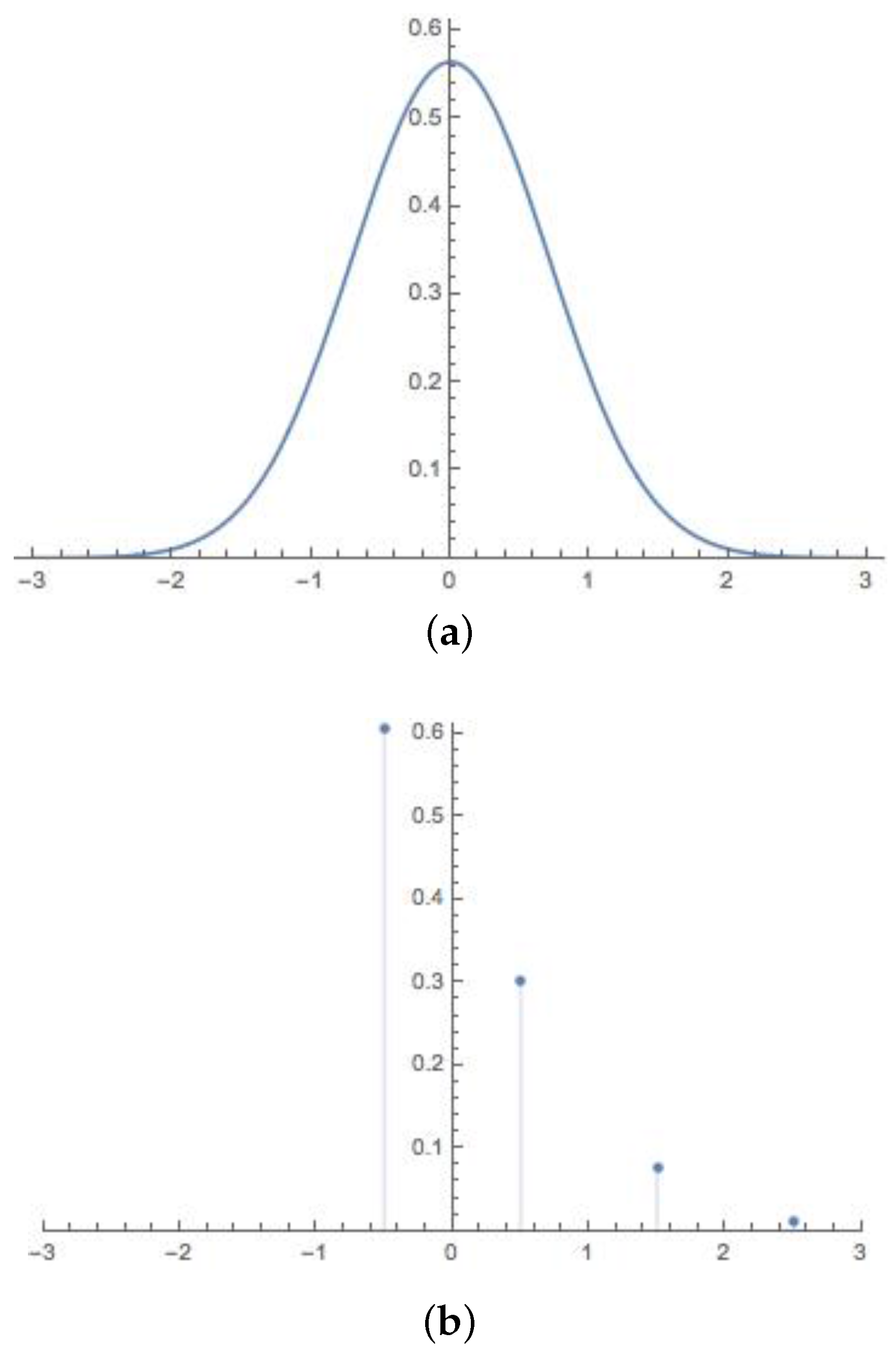
BLW go on to substantiate their criticisms by giving examples of measurements where the O error is zero, even though the distribution of measured values is quite different from the initial state distribution. We will here confine ourselves to their Example 7 in [24]. The reader will easily perceive that a suitably modified version of our discussion applies to their Examples 8, 9 and 10 in [24] (also to Example 5 in [49]). The example is of a measurement of position in which the POVM (positive operator valued measure) describing the distribution of measured values is the spectral measure of the shifted oscillator Hamiltonian
and in which the initial system state is the ground state of . It is easily verified that . On the other hand, it can be seen from Figure 1 that the probability distributions for and are very different. In particular, the distribution for is continuous, whereas that for is discrete. BLW take this to mean that the measurement is highly inaccurate and that the O definition of error is correspondingly misleading. They are right to the extent that there are applications (tomography, for example) for which this measurement would be very ill-suited. However, the purpose of a measurement is not always to accurately reproduce the initial state probability distribution. That is obviously the case in classical physics. Consider, for instance, measurements using a digital ammeter. Here, too, the initial state probability distribution is continuous, while the distribution of measured values is discrete. However, this would not usually be seen as a reason for preferring an analogue meter. The same is true in quantum physics: there are situations where one is only concerned with certain specific features of the distribution of measured values, its detailed shape being otherwise unimportant. Consider, for instance, a state discrimination problem where Bob is promised one of a finite set of N non-overlapping wave-packets localized within the intervals , , and he has to decide which particular wave-packet Alice has sent. In a situation like this, the only important probability is the probability of Bob misidentifying the state that Alice sent. The probability distribution of measured values is irrelevant, except in so far as it has consequences for this failure probability. In particular, there is no reason to prefer a measurement for which the distribution of measured values is continuous. Indeed, it is easily seen that there is a measurement for which the possible pointer values are (with zero corresponding to an input state whose support is disjoint from the interval ) and for which the distribution of measured values is consequently discrete, but having zero failure probability. It is also easy to see that there are measurements with continuous distributions of measured values, more closely approximating the initial state probability distribution in the sense of the Wasserstein two-deviation, but having failure probability greater than zero. Broadly and qualitatively speaking, what one wants in this situation is that the quantity be as small as possible. A measurement like the one described in BLW’s Example 7 satisfies this requirement. The distributions depicted in Figure 1 are indeed very different. However, they have exactly the same mean and variance. Consequently, is not enlarged at all as compared to the initial state variance. This is one of the pieces of information conveyed by the statement that (see inequality (50)), which is not misleading at all, provided it is correctly understood. By contrast, the Wasserstein two-deviation would cause one to prefer, to the measurement depicted in Figure 1, one for which the second distribution was a smeared out version of the first—even though this is likely to be worse for Bob’s particular purposes.
Similarly with the disturbance: in a situation where one is interested in the deviation from the initial state mean, but not in any other feature of the probability distribution, then the D definition, and consequently the O definition of disturbance, will be more useful than the one based on the Wasserstein two-deviation.
It is seldom, if ever, the case, that a single figure of merit captures every potentially relevant feature of a piece of technology. Suppose one is buying a car. If one wants a vehicle that can drive very fast round a carefully prepared track one will choose one figure of merit; if, on the other hand, one wants a vehicle suitable for conveying a family of six to the beach, one will choose another, quite different figure of merit. Similarly with quantum measurements.
In their Examples 7–10, BLW criticize the O definitions on the grounds that the O error can be zero in situations where the initial state and final pointer distributions are very different. In Examples 4 and 6 of Busch et al. [49] and Example 3 of Busch [60], the authors make the opposite point, that the O error can be large in situations where the initial state and final pointer distributions are identical; a fact that they regard as an evident defect of the operator approach. Their argument is based on the principle that a perfectly accurate measurement is one which perfectly reproduces the initial state probability distribution. To see that the principle is not generally valid, consider the following scenario:
Alice lives in a city where of the population is infected with HIV. She is worried that she may have it, so she goes to her doctor Bob to be tested. Bob pulls a coin out of his pocket and tosses it. He then puts on a grave face and says “I am sorry, I have bad news for you.” Alice is outraged, on the grounds that this is not a proper test. Bob, however, insists that it is a proper test. After all, it has the same probability distribution. What more can she want?
This is a classical example. One can easily construct a quantum example. Suppose, for instance, that Alice and Bob are two students who want to perform a test of the Bell inequalities. Unfortunately, they cannot afford state-of-the-art photon counters, so they decide that Alice will toss a fair coin at her station and that Bob will independently toss another fair coin at his. On the principle adopted in Examples 4 and 6 of [49] and Example 3 of [60], these are perfectly accurate measurements. However, they will, of course, fail to reveal any correlations between the two particles.
Outside of the three examples under discussion, Busch and his co-workers adopt a state-independent version of the principle, according to which a measurement is perfectly accurate if it perfectly reproduces the initial state distribution for every initial state. The phrase in italics makes a crucial difference, as can be seen from the following modified version of the doctor scenario (originally suggested by Poulin [61]):
Alice takes 10 cities, in each of which the incidence of HIV is different. She then takes a sample of 100 people from each of these cities and presents them to Bob for testing; without, however, telling Bob which patient comes from which city. It turns out the proportion of positive test results for each city coincides with the actual proportion of HIV-infected people in that city. Alice concludes that, whatever it is that Bob is doing, it probably deserves to be considered a test.
Similarly with the state-independent version of the Busch et al. principle: if a measurement reproduces the initial state distribution for every choice of state, then it is very plausible to argue that it is, in some sense, highly accurate. Calculation confirms that impression. In particular, it is easily seen that a measurement for which the state-independent Wasserstein two-error is zero will successfully reveal the correlations in a Bell experiment.
However, in the examples under discussion, Busch and his co-workers adopt a state-dependent version of the principle. Like the state-dependent version of the operator approach, this version of the principle can easily lead to unreasonable conclusions (cf. the broken-ammeter scenario in Section 2). To show that their objection is not valid, we will focus on Example 3 in [60]. The extension to the other two examples will, we hope, be apparent. We have already discussed this example at the end of Section 3 (specializing to the case of a spin measurement). As we noted there, the O error is non-zero if the initial system state is not an eigenstate of . On the other hand, the fact that the initial system and apparatus states are the same and the fact that the system and apparatus do not interact means that the distribution of measured values is identical to the initial state probability distribution of the measured observable. Busch argues on the basis of this that the measurement is perfectly accurate. The fact that the example is a quantum version of the first doctor scenario may make one suspicious of this conclusion. Busch is, of course, well-aware that the set-up envisaged is not the kind of thing anyone would normally call a measuring apparatus and, indeed, he explicitly draws attention to the fact by comparing it to a broken clock. His point is that a broken clock actually is right twice a day, and he thinks that the same applies to his example. To see that there is an important difference between the two cases, consider a situation where the measured particle is one of a maximally-entangled pair (this differs from the situation we considered in Section 3, where we took it that the measured particle was initially in a pure state). In that case, the C error is non-zero and equal to the O error.
It is (to say the least) questionable whether the process just described counts as a measurement at all. Yet, not only the state-dependent Wasserstein two-error, but also the state-dependent D and C errors are zero. That is not a weakness of the definitions: In all three cases, the fact that the error is zero is a well-defined operational statement, which happens to be true—just as Bob’s statement, in the broken-ammeter scenario, happens to be true. It does, however, illustrate the limitations of state-dependent definitions. We argued in Section 2 that state-dependent definitions have their uses. However, they need to be used with caution. In particular, a state-dependent error is not a figure of merit: its smallness does not, by itself, mean that a measurement is in any sense “good”.
At this point, we ought to stress that, although their arguments are, as it seems to us, invalid, the point that Busch and his co-workers are trying to establish, that there are measurements that are highly accurate as judged by any reasonable operational criterion, but for which the O error is large, could be right. In Section 3, we showed that smallness of the D or C quantities is both necessary and sufficient for a measurement to be accurate or non-disturbing in a well-defined, operational sense. However, in the case of the state-independent O quantities, we only established sufficiency. In the state-dependent case, Korzekwa et al. [59] have shown that there are processes that are completely non-disturbing as judged by any reasonable operational criterion, but for which the state-dependent O disturbance is non-zero (see the discussion at the end of Section 3). However, it remains an open question whether the same is true of the state-dependent O error. The more challenging and, to our mind more important question, of what can be said regarding the state-independent O errors and disturbances, also remains open.
5. Conclusions
In the Introduction, we argued that we need to develop a unified theory of measurement, in which classical measurements are seen as a limiting case of quantum measurements, rather in the way that Newtonian kinematics is a limiting case of relativistic kinematics. In particular, we need an overarching quantum mechanical concept of measurement accuracy that effectively reduces to the classical one in special cases, such as measurements with a meter rule. We argued that, contrary to initial appearances, the Bell-KStheorem is not a major obstacle.
We made a start on the problem by showing that there are at least two ways to reformulate the classical definitions of error and disturbance in a way that does not involve a comparison with pre-existing values. The reformulated definitions have natural quantum generalizations, which we called the D and C definitions. The D and C definitions are examples of quantum definitions that reduce to the classical concept in special cases. They also bound the O quantities introduced in [27,28,29]. They thereby give physical meaning to the O quantities.
We then turned to BLW’s criticisms of the O definitions. We argued that one should not expect there to be a single, canonical way of quantifying the concepts of measurement accuracy and disturbance. The answer to the question “what is the most appropriate quantitative definition?” is always relative to the physical problem of interest. We specified a class of problems for which the D definitions, and consequently, the O definitions, are more appropriate than BLW’s definitions based on the Wasserstein two-deviation.
Our analysis raises a number of questions that might be interesting to investigate. Firstly, in the state-independent case, one would like to know (1) whether the smallness of the O quantities is necessary and sufficient for the corresponding D and C quantities both to be small and (2) whether the smallness of the D quantities is necessary and sufficient for the corresponding C quantities to be small. Secondly, we have seen that there are physical problems for which the D quantities are better-suited than the ones based on the Wasserstein two-deviation. One would like to know if the same is true of the C quantities. Thirdly, it would be interesting to see if the O quantities capture any other operationally well-defined feature of the measurement, in addition to those captured by the D and C quantities. Finally, it would be interesting to see if one can prove error-disturbance and error-error relations expressed in terms of the D and C quantities.
Acknowledgments
We are grateful to Paul Busch, Pekka Lahti, Masanao Ozawa and David Poulin for illuminating discussions. This work was supported by the ARCvia EQuSProject Number CE11001013.
Conflicts of Interest
The author declares no conflict of interest.
Appendix A. Proof of Inequalities (13), (14), (17) and (18)
In [27], we gave a proof of inequalities (13), (14), (17) and (18), which skated over certain questions of domain and differentiability. Our proof has since been criticized for its lack of rigour. We here take the opportunity to fill in the missing details. We incidentally strengthen the statement of inequalities (17) and (18) slightly.
The problem we face is that the operators , are not defined on the whole Hilbert space. Specifically, is in the domain of if and only if the function is integrable. The domain of is defined similarly. Expressed more intuitively: is in the domain of if and only if . We take the view that states for which that is not true are never realized in a real, Earthbound laboratory experiment. To put it more succinctly: they are unphysical.
One’s first thought may be that one can define the domain of physical states to be the set of all , such that (respectively, ) is zero for all x, such that (respectively, all p, such that ), for suitably large positive constants , . However, the set of such states is empty (because, if is zero outside the interval , then its Fourier transform is analytic, by Schwartz’s extension of the Paley–Wiener theorem [see, for example, Treves [62]]). Nevertheless, although the theory forces at least one of the wave-functions , to have an infinite tail, nothing observable under ordinary laboratory conditions can depend on it. It is not possible that a currently performable laboratory experiment can give rise to a state in which there is a significant probability of the momentum being greater than , and even if it were possible, one would not use non-relativistic quantum mechanics to describe it; nor is it possible to produce states for which there is a significant probability of being greater than . We need to give quantitative expression to this point, that the infinite tails are physically irrelevant. We accordingly take the view (inspired by the rigged Hilbert space formulation of quantum mechanics [63,64,65]) that the set of physical pure states consists of those states for which the position space wave function is (a) and (b) rapidly decreasing at infinity in the sense that
for every pair of non-negative integers n, m (in other words, is a test function for the space of tempered distributions [62]). Note that this is equivalent to requiring that the momentum space wave function is and rapidly decreasing at infinity. Note also that is in the domain of every monomial in and .
At first sight, this definition may appear arbitrary. The reader may allow that it is reasonable to impose some restriction on the behaviour at infinity, but wonder why we make this particular choice. Indeed, the requirement is much stronger than we need for our present purposes. We make the definition nonetheless because actually it is not arbitrary, as can be seen by using a von Neumann lattice [9,66,67]. For some appropriate scale-length λ, let be the coherent state with wave function
Then, the set with one point removed is a basis. Choose some suitably enormous integer N, and let be the projector onto the finite dimensional subspace spanned by the set . Then, for any state that is relevant to a real laboratory experiment, the quantity will be negligible. Consequently, predictions obtained using the state will be experimentally indistinguishable from ones obtained using the state
Without loss of predictive power, we may therefore replace with . The fact that is a finite linear combination of coherent states means that it belongs to . Of course, also includes states like with n, m both much larger than N, which are certainly not relevant to ordinary, Earthbound laboratory experiments (being localized outside the cosmic event horizon). The point is only that every pure state that is experimentally relevant is empirically indistinguishable from a state in .
Finally, we need to define , the set of physical density matrices. For each non-negative integer m and real β, define norms
Now, let
be an arbitrary density matrix with eigenvectors . We define to consist of those for which for all n and for which
for all m, β. Note that it is enough to demand that one set of suprema is finite, since the finiteness of the other is then automatic. Note also that in the case when the spectrum of has degeneracies, the finiteness of the suprema does not depend on the particular choice of eigenvectors. Finally, let us remark that for the technical purposes of this Appendix, it would be enough to require that the suprema are finite for the particular case , .
This definition is justified by the fact that no experimentally relevant density matrix can be distinguished empirically from a state in . Indeed, let be an experimentally relevant density matrix, and let be the projector onto the first N eigenstates. Choose N so that is smaller than some suitably tiny number. No practicable experiment can distinguish between and . By the argument we used to justify the definition of , the state is in turn empirically indistinguishable from one of the form
where the states are a finite orthonormal set in . The fact that the set is finite means .
The proof of the main theorem depends on three technical lemmas. Define displacement operators
and, for each , let
It is easily seen that for all x, p.
Lemma 1.
For all , the function is differentiable in the sense that
for all x, p, all , where B is a fixed positive constant independent of .
Proof.
It is easily seen that
where
Hence
The second inequality is proved in the same way. ☐
Lemma 2.
For all , , , are uniformly continuous on every compact subset of . Specifically, let be such a set. Then
for all , , where , , and where the are positive constants that depend on , but not on .
Proof.
The first inequality is a straightforward consequence of Lemma 1 and the inequalities
To prove the second inequality, let . Then
implying
The proof now reduces to an application of the first inequality. The last inequality is proved in the same way. ☐
Let the initial apparatus state be
for some set of positive numbers and orthonormal set . We argue on the same physical grounds adduced in the first few paragraphs of this Appendix that the quantities , are well defined for all . Finally, for given positive real numbers , , define to be the phase-space box consisting of all , such that , .
Lemma 3.
Let be any element of , and let . Let be any self-adjoint operator, such that , are defined, and , , are both defined and bounded on . Then, is differentiable on , and
Moreover, the derivatives are uniformly continuous on .
Proof.
Lemmas 1 and 2 also imply
The uniform continuity of the x derivative now follows by another application of the Cauchy–Schwartz inequality. The uniform continuity of the p derivative is proved similarly. ☐
We are now ready to prove our main result.
Theorem 4.
Let be a subset of containing at least one state ρ, such that
for all . Then
for every measurement of position, and
for every joint measurement of position and momentum.
Proof.
To prove the first relation, observe that it is automatic if either of the quantities , is infinite. Suppose, on the other hand, they are both finite. It is easily seen that
Let be any state in satisfying condition (A39). It is easily seen that , are bounded. Therefore, we can apply Lemma 3 with to deduce
where and
Since is continuous, it is integrable. Hence
where is the boundary of and is the outward-pointing normal. The second inequality is proved in the same way, starting from the commutation relation
☐
Inequalities (13), (14) are proved by specializing to the case and taking the limit as , .
References
- Heisenberg, W. Über den anschaulichen Inhalt der quantentheoretischen Kinematik und Mechanik. Zeitschrift für Physik 1927, 43, 172–198. (In German) [Google Scholar] [CrossRef]
- Busch, P.; Lahti, P.; Werner, R.F. Measurement uncertainty relations. J. Math. Phys. 2014, 55, 042111. [Google Scholar] [CrossRef]
- Bell, J.S. On the problem of hidden variables in quantum mechanics. Rev. Mod. Phys. 1966, 38, 447–452. [Google Scholar] [CrossRef]
- Kochen, S.; Specker, E. The problem of hidden variables in quantum mechanics. J. Math. Mech. 1967, 17, 59–87. [Google Scholar] [CrossRef]
- Clifton, R.; Kent, A. Simulating quantum mechanics by non-contextual hidden variables. Proc. Roy. Soc. Lond. A 2000, 456, 2101–2114. [Google Scholar] [CrossRef]
- Appleby, D.M. The Bell-Kochen-Specker Theorem. Stud. Hist. Philos. Mod. Phys. 2005, 36, 1–28. [Google Scholar] [CrossRef]
- Bell, J.S. On the impossible pilot wave. Found. Phys. 1982, 12, 989–999. [Google Scholar] [CrossRef]
- Heisenberg, W. The Physical Principles of the Quantum Theory; University of Chicago Press: Chicago, IL, USA, 1930. [Google Scholar]
- Von Neumann, J. Mathematische Grundlagen der Quantenmechanik; Springer: Berlin, Germany, 1932. [Google Scholar] English Translation Published as Mathematical Foundations of Quantum Mechanics; Beyer, R.T., Translator; Princeton University Press: Princeton, NJ, USA, 1955.
- Kennard, E. Zur quantenmechanik einfacher bewegungstypen. Zeitschrift fü Physik 1927, 44, 326–352. (In German) [Google Scholar] [CrossRef]
- Weyl, H. Gruppentheorie und Quantenmechanik; Hirzel, 1928. [Google Scholar] English Translation of the Revised Second Edition Published as The Theory of Groups and Quantum Mechanics; Robertson, H.P., Translator; Dover Publications: New York, NY, USA, 1950.
- Robertson, H.P. The uncertainty principle. Phys. Rev. 1929, 34, 163–164. [Google Scholar] [CrossRef]
- Schrödinger, E. Um Heisenbergschen Unschärfeprinzip. Sitzungsberichte der Preussischen Akademie der Wissenschaften Physikalisch-Mathematische Klasse 1930, 14, 296–303. (In German) [Google Scholar]
- Busch, P.; Heinonen, T.; Lahti, P. Heisenberg’s uncertainty principle. Phys. Rep. 2007, 452, 155–176. [Google Scholar] [CrossRef] [Green Version]
- Arthurs, E.; Kelly, J.L. On the simultaneous measurement of a pair of conjugate observables. Bell Syst. Tech. J. 1965, 44, 725–729. [Google Scholar] [CrossRef]
- Bell, J.S. Speakable and unspeakable in quantum mechanics. In Speakable and Unspeakable in Quantum Mechanics; Cambridge University Press: Cambridge, UK, 1987; pp. 169–172. [Google Scholar]
- Howard, D. Who invented the “Copenhagen interpretation”? A study in mythology. Philos. Sci. 2004, 71, 669–682. [Google Scholar] [CrossRef]
- Camilleri, K. Heisenberg and the Interpretation of Quantum Mechanics; Cambridge University Press: Cambridge, UK, 2009. [Google Scholar]
- Faye, J. Copenhagen interpretation of quantum mechanics. In The Stanford Encyclopedia of Philosophy; Zalta, E.N., Ed.; Stanford University: Stanford, CA, USA, 2014. [Google Scholar]
- Braginsky, V.B.; Vorontsov, Y.I.; Thorne, K.S. Quantum nondemolition measurements. Science 1980, 209, 547–557. [Google Scholar] [CrossRef] [PubMed]
- Braginsky, V.B.; Khalili, F.Y. Quantum Measurement; Cambridge University Press: Cambridge, UK, 1992. [Google Scholar]
- Plotnitsky, A. Niels Bohr and Complementarity: An Introduction; Springer Briefs in Physics; Springer: Berlin, Germany, 2013. [Google Scholar]
- Busch, P.; Lahti, P.; Werner, R.F. Proof of Heisenberg’s error-disturbance relation. Phys. Rev. Lett. 2013, 111, 160405. [Google Scholar] [CrossRef] [PubMed]
- Busch, P.; Lahti, P.; Werner, R.F. Colloquium: Quantum root-mean-square error and measurement uncertainty relations. Rev. Mod. Phys. 2014, 86, 1261–1281. [Google Scholar] [CrossRef]
- Busch, P.; Lahti, P.; Werner, R.F. Measurement uncertainty: Reply to critics. 2014. arXiv:1402.3102. Available online: http://arxiv.org/abs/1402.3102 (accessed on 29 April 2016).
- Busch, P.; Lahti, P.; Werner, R.F. Comment on “Experimental Test of Error-Disturbance Uncertainty Relations by Weak Measurement”. 2014. arXiv:1403.0367. Available online: http://arxiv.org/abs/1403.0367 (accessed on 29 April 2016).
- Appleby, D.M. Error principle. Int. J. Theor. Phys. 1998, 37, 2557–2572. [Google Scholar] [CrossRef]
- Ozawa, M. Universally valid reformulation of the Heisenberg uncertainty principle on noise and disturbance in measurement. Phys. Rev. A 2003, 67, 042105. [Google Scholar] [CrossRef]
- Ozawa, M. Physical content of Heisenberg’s uncertainty relation: Limitation and reformulation. Phys. Lett. A 2003, 318, 21–29. [Google Scholar] [CrossRef]
- Ozawa, M. Disproving Heisenberg’s error-disturbance relation. 2013. arXiv:1308.3540. Available online: http://arxiv.org/abs/1308.3540 (accessed on 29 April 2016).
- Ozawa, M. Heisenberg’s uncertainty relation: Violation and reformulation. In Proceedings of the Second International Symposium on Emergent Quantum Mechanics, Vienna, Austria, 3–6 October 2013; Volume 504, p. 012024.
- Appleby, D.M. Concept of experimental accuracy and simultaneous measurements of position and momentum. Int. J. Theor. Phys. 1998, 37, 1491–1509. [Google Scholar] [CrossRef]
- Appleby, D.M. Maximal accuracy and minimal disturbance in the Arthurs-Kelly simultaneous measurement process. J. Phys. A 1998, 31, 6419–6436. [Google Scholar] [CrossRef]
- Appleby, D.M. Optimal joint measurements of position and momentum. Int. J. Theor. Phys. 1999, 38, 807–825. [Google Scholar] [CrossRef]
- Arthurs, E.; Goodman, M.S. Quantum correlations: A generalized Heisenberg uncertainty relation. Phys. Rev. Lett. 1988, 60, 2447–2449. [Google Scholar] [CrossRef] [PubMed]
- Yuen, H.P. Generalized quantum measurements and approximate simultaneous measurements of noncommuting observables. Phys. Lett. A 1982, 91, 101–104. [Google Scholar] [CrossRef]
- Ishikawa, S. Uncertainty relations in simultaneous measurements for arbitrary observables. Rep. Math. Phys. 1991, 29, 257–273. [Google Scholar] [CrossRef]
- Ozawa, M. Quantum limits of measurements and uncertainty principle. In Proceedings of the Quantum Aspects of Optical Communications: Proceedings of a Workshop, Paris, France, 26–28 November 1990; Volume 378.
- Ozawa, M. Position measuring interactions and the Heisenberg uncertainty principle. Phys. Lett. A 2002, 299, 1–7. [Google Scholar] [CrossRef]
- Ozawa, M. Uncertainty principle for quantum instruments and computing. Int. J. Quantum Inf. 2003, 1, 569–588. [Google Scholar] [CrossRef]
- Ozawa, M. Uncertainty relations for joint measurements of noncommuting observables. Phys. Lett. A 2004, 320, 367–374. [Google Scholar] [CrossRef]
- Hall, M.J.W. Prior information: How to circumvent the standard joint-measurement uncertainty relation. Phys. Rev. A 2004, 69, 052113. [Google Scholar] [CrossRef]
- Weston, M.M.; Hall, M.J.W.; Palsson, M.S.; Wiseman, H.M.; Pryde, G.J. Experimental test of universal complementarity relations. Phys. Rev. Lett. 2013, 110, 220402. [Google Scholar] [CrossRef] [PubMed]
- Branciard, C. Deriving tight error-trade-off relations for approximate joint measurements of incompatible quantum observables. Phys. Rev. A 2014, 89, 022124. [Google Scholar] [CrossRef]
- Ozawa, M. Error-disturbance relations in mixed states. 2014. arXiv:1404.3388. Available online: http://arxiv.org/abs/1404.3388 (accessed on 29 April 2016).
- Rozema, L.A.; Mahler, D.H.; Hayat, A.; Steinberg, A.M. A note on different definitions of momentum disturbance. Quantum Stud. Math. Found. 2015, 2, 17–22. [Google Scholar] [CrossRef]
- Fuchs, C.A.; Schack, R. Quantum-Bayesian Coherence. Rev. Mod. Phys. 2013, 85, 1693–1715. [Google Scholar] [CrossRef]
- Ozawa, M. Uncertainty relations for noise and disturbance in generalized quantum measurements. Ann. Phys. 2004, 311, 350–416. [Google Scholar] [CrossRef]
- Busch, P.; Heinonen, T.; Lahti, P. Noise and disturbance in quantum measurement. Phys. Lett. A 2004, 320, 261–270. [Google Scholar] [CrossRef]
- Born, M. Zur Quantenmechanik der Stoßorgänge. Zeitschrift fü Physik 1926, 37, 863–867. (In German) [Google Scholar] [CrossRef]
- Wheeler, J.A.; Zurek, W.H. (Eds.) Quantum Theory and Measurement; Princeton University Press: Princeton, NJ, USA, 1983.
- Werner, R.F. The uncertainty relation for joint measurement of postion and momentum. Quantum Inf. Comput. 2004, 4, 546–562. [Google Scholar]
- Appleby, D.M. Optimal measurements of spin direction. Int. J. Theor. Phys. 2000, 39, 2231–2252. [Google Scholar] [CrossRef]
- Bohm, D.; Hiley, B. The Undivided Universe: An Ontological Interpretation of Quantum Theory; Routledge: Abingdon, UK, 1993. [Google Scholar]
- Holland, P.R. The Quantum Theory of Motion; Cambridge University Press: Cambridge, UK, 1993. [Google Scholar]
- Appleby, D.M. Generic Bohmian trajectories of an isolated particle. Found. Phys. 1999, 29, 1863–1883. [Google Scholar] [CrossRef]
- Appleby, D.M. Bohmian trajectories post-decoherence. Found. Phys. 1999, 29, 1885–1916. [Google Scholar] [CrossRef]
- Çinlar, E. Probability and Stochastics; Graduate Texts in Mathematics No. 261; Springer: Berlin, Germany, 2011. [Google Scholar]
- Korzekwa, K.; Jennings, D.; Rudolph, T. Operational constraints on state-dependent formulations of quantum error-disturbance trade-off relations. Phys. Rev. A 2014, 89, 052108. [Google Scholar] [CrossRef]
- Busch, P. Quantum rms error and Heisenberg’s error-disturbance relation. In Proceedings of the Wigner 111—Colourful and Deep Scientific Symposium, Budapest, Hungary, 11–13 November 2013.
- Poulin, D. Université de Sherbrooke, Québec, Canada. Personal Communication, 2014. [Google Scholar]
- Treves, F. Topological Vector Spaces, Distributions and Kernels; Academic Press: Cambridge, MA, USA, 1967. [Google Scholar]
- Gel’fand, I.M.; Vilenkin, N.Y. Generalized Functions: Applications of Harmonic Analysis; Academic Press: Cambridge, MA, USA, 1964; Volume 4. [Google Scholar]
- Böhm, A. The Rigged Hilbert Space and Quantum Mechanics; Lecture Notes in Physics, No. 78; Springer: Berlin, Germany, 1978. [Google Scholar]
- Böhm, A.; Gadella, M. Dirac Kets, Gamow Vectors and Gel’fand Triplets; Lecture Notes in Physics, No. 348; Springer: Berlin, Germany, 1989. [Google Scholar]
- Perelomov, A.M. On the completeness of a system of coherent states. Theor. Math. Phys. 1971, 6, 156–164. [Google Scholar] [CrossRef]
- Bargmann, V.; Butera, P.; Girardello, L.; Klauder, J.R. On the completeness of the coherent states. Rep. Math. Phys. 1971, 2, 221–228. [Google Scholar] [CrossRef]
Figure 1.
Probability distributions for (a) and (b) in Busch, Lahti and Werner’s (BLW) Example 7 (units chosen so that ).
Figure 1.
Probability distributions for (a) and (b) in Busch, Lahti and Werner’s (BLW) Example 7 (units chosen so that ).

© 2016 by the author; licensee MDPI, Basel, Switzerland. This article is an open access article distributed under the terms and conditions of the Creative Commons Attribution (CC-BY) license (http://creativecommons.org/licenses/by/4.0/).
Share and Cite
MDPI and ACS Style
Appleby, D.M. Quantum Errors and Disturbances: Response to Busch, Lahti and Werner. Entropy 2016, 18, 174. https://0-doi-org.brum.beds.ac.uk/10.3390/e18050174
AMA Style
Appleby DM. Quantum Errors and Disturbances: Response to Busch, Lahti and Werner. Entropy. 2016; 18(5):174. https://0-doi-org.brum.beds.ac.uk/10.3390/e18050174
Chicago/Turabian StyleAppleby, David Marcus. 2016. "Quantum Errors and Disturbances: Response to Busch, Lahti and Werner" Entropy 18, no. 5: 174. https://0-doi-org.brum.beds.ac.uk/10.3390/e18050174
Note that from the first issue of 2016, this journal uses article numbers instead of page numbers. See further details here.